Universitat de - Departament d'Astronomia i Meteorologia ...

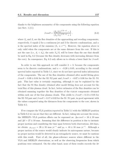
6.3. Results and discussion 157
thanks to the brightness asymmetry of the components using the following equation
(see Sect. 1.2.1):
β cos θ = (Sa/Sr) 1/(k−α) − 1
(Sa/Sr) 1/(k−α) + 1
, (6.2)
where Sa and Sr are the flux densities of the approaching and receding components,
respectively, k equals 2 for a continuous jet and 3 for discrete condensations, and α
is the spectral index of the emission (Sν ∝ ν +α ). However, the equation above is
only valid when the components are at the same distance from the core. If this is
not the case (i.e., dr < da), the ratio Sa/Sr will be lower than the one that should
be used in Eq. 6.2 (because the flux density decreases with increasing distance from
the core). In consequence, Eq. 6.2 only allows us to obtain a lower limit for β cos θ.
In order to use this approach we will consider k = 3, because the components
seem to be discrete condensations, and α = −0.20 ± 0.05, according to the overall
spectral index reported in Table 5.1, since we do not have spectral index information
of the components. The use of the flux densities obtained after model fitting gives
β cos θ > 0.09 ± 0.04 for the S2–N2 pair and β cos θ > −0.07 ± 0.08 for the S1–N1
pair. This last value is certainly surprising, although it can be explained by the
fact that the S1 flux density obtained after model fitting does not account for the
total flux of this plasma cloud. In fact, better estimates of the flux densities can be
obtained summing together the flux densities of the clean components obtained
within each one of the four plasma clouds. This yields to β cos θ > 0.13 ± 0.05 for
the S2–N2 pair and β cos θ > 0.17±0.02 for the S1–N1 pair, in good agreement with
the values computed using the distances from the components to the core, shown in
Table 6.5.
If we compare the VLA position reported in Table 5.1 with the MERLIN position
in Table 6.2 we can see that they are different. In fact, taking into account the errors,
the MERLIN−VLA position offsets can be expressed as: ∆α cos δ = 16 ± 10 mas
and ∆δ = 27 ± 10 mas. Assuming that the difference in position is due to intrinsic
proper motions and considering the time span between both observations, 224 days,
we obtain: µα cos δ = 26 ± 16 mas yr −1 and µδ = 44 ± 16 mas yr −1 . Although a
proper motion of the source would clearly indicate its microquasar nature, because
no proper motion would be detected in an extragalactic source, we must be cautious
with this result. First of all, the phase-reference sources where different in the
VLA and MERLIN observations, as well as the observing frequencies from which
positions were estimated. On the other hand, none of these results exceeds the 3σ