Prakties 2 - Electrical, Electronic and Computer Engineering

Departement Elektriese,
Elektroniese en Rekenaar-
Ingenieurswese
Prakties 2:
Ontwerp en realisering
van PID beheerders
Kopiereg voorbehou
Beheerstelsels
EBB320
Department of Electrical,
Electronic and Computer
Engineering
Practical 2:
Design and realisation of
PID controllers
Copyright reserved
Control Systems
EBB320
Compiled by Hein Swart and Prof F. R. Camisani-Calzolari. Updated by Björn Matthews
1. Introduction
The aim of this practical is to design and build PID controllers to control the system built in Practical 1.
2. Background
A basic knowledge of the following is needed:
1. Cohen-Coon tuning by using the process reaction curve (p.169 in Goodwin et al., (2001))
2. Ziegler-Nichols oscillation method (p.162 in Goodwin et al., (2001) or p.317 in Seborg et al.,
(2004))
3. Bode stability criterion (p.365 in Seborg et al., (2004))
A short description of each of these topics is given next. Please refer to references for more complete
descriptions.
2.1 Cohen-Coon process reaction curve method
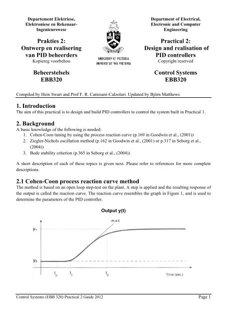
The method is based on an open loop step-test on the plant. A step is applied and the resulting response of
the output is called the reaction curve. The reaction curve resembles the graph in Figure 1, and is used to
determine the parameters of the PID controller.
y∞
y0
Output y(t)
Control Systems (EBB 320) Practical 2 Guide 2012 Page 1

Figure 1. Reaction curve (m.s.t = maximum slope tangent. Reproduced from Goodwin et al., (2001))
The values for , and are read off from the reaction curve where is the time at which the step was
applied, is the time at which the system starts to react and is the time where the maximum slope
tangent (drawn from ) intercepts the steady state output value. Once , and have been
determined from the graph, the dead time, approximate time constant and gain are calculated. The dead
time of the system is calculated as . The approximate time constant is and the
gain is calculated as:
where is the output and is the input. These values are then substituted into the equations from the
following table to determine the PID parameters.
[
]
( )
Table 1: Controller settings for the Cohen-Coon process reaction curve method
The standard form for the PID controller is given by:
( ) (
Note that the values in Table 1 (and Table 2) are given for the standard PID controller form.
2.2 Ziegler-Nichols oscillation method
This method is described in Seborg et al., (2004) as follows:
1. After the process has reached steady state, eliminate the integral and derivative action (i.e.
implement proportional only control).
2. Set the controller gain to a small non-zero value.
3. Introduce a small momentary set-point change and observe the output. Gradually increase the
controller gain and repeat the introduction of the momentary set-point change until sustained
oscillation is seen at the output. The oscillation at the output should have a constant amplitude (i.e.
it should not die out over time). The numerical value of the proportional controller gain that
produces the continuous oscillation is called the ultimate gain . The period of the oscillation is
called the ultimate period .
4. Calculate the PID controller settings from the Ziegler-Nichols tuning settings table.
Ziegler-Nichols Method
PID
Table 2: Controller settings based on the Ziegler-Nichols oscillation method
Control Systems (EBB 320) Practical 2 Guide 2012 Page 2
)

The numeric value for the ultimate controller gain may be calculated from the method of Goodwin et al.,
(2001) (p.162) or from the Bode stability criterion (in Seborg p.317, (2004)).
2.3 Bode stability criterion
The Bode stability criterion is a method to evaluate the stability of a system containing time delays. There
is a host of applications for this method but all we are interested in is the calculation of the ultimate
controller gain that leads to sustained oscillation. This gain is achieved at the point where the system is
marginally stable. From the Bode stability criterion this is the point where or equivalently
| | and . Here is the open loop transfer function. In our case it is simply the
product of the proportional controller and the plant transfer function (first order plus time delay).
Rewrite the open loop transfer function into magnitude and phase form. Determine the frequency at
which the phase becomes . At this frequency the magnitude must equal 1 for marginal stability.
Substitute the calculated frequency back into the magnitude equation and solve for the ultimate controller
gain.
3. Additional circuits
The controller ( ) can be written in the following form:
( ) ( )
( ) [(
Note that you will need to rewrite the standard PID controller form, given in section 2.1, into this form to
calculate the component values.
Figure 1: Realization of controller ( ( )).
Control Systems (EBB 320) Practical 2 Guide 2012 Page 3
)
⁄
]

Figure 2: Realisation of controller with and represented by resistors and capacitors.
The implementation of the controller is shown in Figure 1 and Figure 2.
4. Closed Loop System
The closed loop system is shown in Figure 3 and can be implemented as in Figure 4.
Figure 3: The closed loop system.
Figure 4: The closed loop system for practical implementation.
The summation function can be implemented as in Figure 5. Set . is the feedback signal,
is the set point input and is the input of the controller.
Control Systems (EBB 320) Practical 2 Guide 2012 Page 4

Figure 5: The implementation of the summation function.
5. Preparation
All pre-assignments must be done in the lab book (of each student) and will be marked during the
practical session. Each member of the group must participate in the preparation.
1. Design (i.e. calculate the tuning parameters) a PID controller by simulating the step response of
the plant of practical 1, and making use of the Cohen-Coon reaction curve method. Use the system
with the Padé approximation applied.
2. Design a PID controller from the Ziegler-Nichols oscillation method by theoretically calculating
the ultimate controller gain and ultimate oscillation period from the transfer function of the
system. Use the system with the Padé approximation applied.
3. Compute the capacitor and resistor values for each of the designed PID controllers.
4. Simulate the closed loop system using both controllers (see Figure 4). Measure the peak time ( ),
percentage overshoot ( ) and steady-state-error from each simulation.
(Note that the simulations may be done in PSpice or Simulink. The setup and the results of each
simulation should be explicitly indicated.)
6. Lab assignments
1. Build the Cohen-Coon controller you designed in 5.1 (use own components!).
2. Measure (look on oscilloscope) the system the peak time ( ), percentage overshoot ( ) and
steady-state-error and compare this with the controller from your simulated response. The
definitions of these quantities may be found from Nise, (2008).
(Note: Please build the Cohen-Coon and Ziegler-Nichols controllers separately such that they can be
interchanged easily in the demo. They should however be implemented on the same plant).
3. Build the Ziegler-Nichols controller (as designed in 5.2).
4. Measure , and the steady-state-error for the system with the Ziegler-Nichols controller
implemented, and compare this with the simulation results found in 5.4.
Control Systems (EBB 320) Practical 2 Guide 2012 Page 5

7. Report
The report must be written in English and include the following:
1. Design of the PID controller with the Cohen-Coon method.
2. Design of the controller with the Ziegler-Nichols oscillation method.
3. Component values calculated for realisation of the controllers.
4. The measured , and steady-state-error values from the simulations as well as from the
practical results.
5. Comparison of these values for the simulation and practically implemented controllers.
6. PSpice or Simulink simulation of the closed loop systems.
7. Discussion of results.
8. A conclusion.
8. Demo
The demo will be based on the following:
1. Lab books with completed preparation assignments.
2. Closed loop response of the implemented Cohen-Coon based PID controller.
3. Closed loop response of the implemented Ziegler-Nichols based PID controller.
4. Performance measures achieved ( , and steady-state-error) for the practical controllers.
5. Answering of questions.
(Note: Please build the Cohen-Coon and Ziegler-Nichols controllers separately such that they can be
interchanged easily in the demo. They should however be implemented on the same plant).
9. References
[1] Goodwin, G.C., Graebe, S.F., Salgado, M.E., Control System Design, 2001, Prentice Hall.
[2] Seborg, D.E., Edgar, T.F., Mellichamp, D.A, Process Dynamics and Control, 2004, Wiley.
[3] Norman S. Nise, Control Systems Engineering, 5th Ed., 2008, John Wiley & Sons.
Control Systems (EBB 320) Practical 2 Guide 2012 Page 6