Orbital Maneuvers - Orbital and Celestial Mechanics Website
Orbital Maneuvers - Orbital and Celestial Mechanics Website
Orbital Maneuvers - Orbital and Celestial Mechanics Website

You also want an ePaper? Increase the reach of your titles
YUMPU automatically turns print PDFs into web optimized ePapers that Google loves.
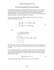
<strong>Orbital</strong> <strong>Mechanics</strong> with MATLAB<br />
<strong>Orbital</strong> <strong>Maneuvers</strong><br />
This document describes several MATLAB scripts that can be used to determine the<br />
characteristics of impulsive <strong>and</strong> finite burn maneuvers that modify orbits. The first script<br />
calculates the impulsive V required to change a circular orbit, the second script determines the<br />
single impulse required to maneuver between any two intersecting orbits, <strong>and</strong> a third MATLAB<br />
script models a finite burn orbit transfer between two coplanar elliptical orbits. The impulsive<br />
V assumption means that the velocity, but not the position, of the space vehicle is changed<br />
instantaneously.<br />
This software suite also includes scripts that determine the characteristics of low-thrust orbital<br />
transfer, the impulsive maneuvers required to de-orbit from circular <strong>and</strong> elliptic orbits, <strong>and</strong> a<br />
script that calculates the characteristics of coplanar aero-assisted orbital transfer. A script to<br />
solve both the coplanar <strong>and</strong> non-coplanar Hohmann orbit transfer is also included along with<br />
scripts that perform a primer vector analysis of two impulse, coplanar Hohmann transfers <strong>and</strong><br />
phasing or rendezvous maneuvers.<br />
maneuver1.m – circular orbit plane change<br />
This section describes the geometry <strong>and</strong> equations associated with single impulse maneuvers that<br />
modify the inclination <strong>and</strong>/or right ascension of the ascending node (RAAN) of circular orbits.<br />
The following diagram illustrates the geometry of this type of maneuver.<br />
In this picture the orbital inclinations of the initial <strong>and</strong> final orbits are i i <strong>and</strong> i f , respectively. The<br />
RAAN of the initial orbit is i <strong>and</strong> f is the RAAN of the final orbit. The right ascension of<br />
the ascending node of an orbit is measured from the inertial x-axis along the equator in the<br />
direction of the Earth's rotation. From spherical trigonometry relationships is the angle<br />
between the two orbit planes.<br />
The next diagram illustrates the possible points of intersection. From this ground track<br />
schematic we can see that there are two pairs of orbit intersections on both the initial <strong>and</strong> final<br />
orbits which depend on the relative RAAN between these two orbits.<br />
page 1
<strong>Orbital</strong> <strong>Mechanics</strong> with MATLAB<br />
The total plane change angle due to the modification of inclination <strong>and</strong> RAAN can be expressed<br />
as<br />
1 cos siniisinif cos f icosiicosi <br />
<br />
<br />
f <br />
We can define an index imp that depends on the sign of the RAAN change f i<br />
as<br />
follows:<br />
If 0 then imp = 1 <strong>and</strong> 3<br />
or<br />
If 0 then imp = 2 <strong>and</strong> 4.<br />
final orbit<br />
imp=1 imp=2<br />
equator<br />
It is convenient to define the location of impulses by their argument of latitude. The argument of<br />
latitude is the angle from the ascending node, measured along the orbital plane, to the point of<br />
interest. The argument of latitude is equal to the sum of the argument of perigee <strong>and</strong> true<br />
anomaly. Since for circular orbits there is no argument of perigee, the argument of latitude <strong>and</strong><br />
true anomaly are identical.<br />
The two possible arguments of latitude on the initial orbit depend on the values of imp as<br />
follows:<br />
integer / 2 1 imp<br />
u imp u<br />
i<br />
<br />
where u is the impulse argument of latitude on the initial orbit given by<br />
u<br />
imp=3<br />
cosi sini cos<br />
<br />
1<br />
i f<br />
cos <br />
sinii sin<br />
<br />
We can determine the argument of latitude of an impulse on the final orbit by forming the unit<br />
position vectors from the ascending node to the impulse. The argument of latitude of the first<br />
opportunity on the final orbit is given by<br />
page 2<br />
initial orbits<br />
imp=4
<strong>Orbital</strong> <strong>Mechanics</strong> with MATLAB<br />
u<br />
U U <br />
1<br />
cos 1 2<br />
where U 1 is the unit position vector of the impulse on the initial orbit <strong>and</strong> U 2 is the unit position<br />
vector to the ascending node of the final orbit. The argument of latitude of the second impulse<br />
opportunity on the final orbit is equal to 180 degrees plus this value.<br />
The maneuver V vector is given by the vector difference between the velocity vectors of the<br />
initial <strong>and</strong> final orbits as follows:<br />
V VfV i<br />
These velocity vectors are evaluated at the points of orbital intersection. The scalar magnitude of<br />
the V is determined from the components of this vector according to<br />
V V V V<br />
2 2 2<br />
x y z<br />
For the case where there is no RAAN change, the two impulse locations occur at the common<br />
ascending <strong>and</strong> descending nodes of both the initial <strong>and</strong> final orbits. The arguments of latitude of<br />
these two orbital points are 0 <strong>and</strong> 180 degrees, respectively.<br />
The required V can also be determined using vector manipulation. Unit vectors normal to<br />
each orbit plane can be defined as follows:<br />
siniisin i<br />
<br />
ni<br />
<br />
<br />
siniicos <br />
i<br />
cosii<br />
<br />
n<br />
sini f sin f <br />
<br />
<br />
<br />
sini cos<br />
<br />
<br />
cosi<br />
f <br />
f f f<br />
A unit vector along the intersection of the initial <strong>and</strong> final orbit planes is given by<br />
n n<br />
m <br />
n n<br />
f i<br />
f i<br />
The velocity vector prior to the maneuver is calculated from<br />
n m<br />
V V<br />
i<br />
i<br />
nim lc<br />
The velocity vector after the maneuver is given by<br />
page 3
<strong>Orbital</strong> <strong>Mechanics</strong> with MATLAB<br />
V<br />
n m<br />
V<br />
f<br />
f<br />
n f m<br />
lc<br />
where V lc is the local circular velocity at the maneuver altitude.<br />
Finally, the maneuver V vector is determined from<br />
V VfV i<br />
The equations described here have been implemented in an interactive MATLAB script called<br />
maneuver1.m. This script will prompt you for the altitude, inclination <strong>and</strong> RAAN of both the<br />
initial <strong>and</strong> final orbits. A typical user interaction with this script is as follows.<br />
program maneuver1<br />
< one impulse transfer between circular orbits ><br />
initial orbit<br />
please input the altitude (kilometers)<br />
(altitude > 0)<br />
? 185<br />
please input the orbital inclination (degrees)<br />
(0
solution # 1<br />
<strong>Orbital</strong> <strong>Mechanics</strong> with MATLAB<br />
initial orbit true anomaly 44.4493 degrees<br />
final orbit true anomaly 28.2000 degrees<br />
delta-V required 2733.7882 meters/second<br />
solution # 2<br />
initial orbit true anomaly 224.4493 degrees<br />
final orbit true anomaly 208.2000 degrees<br />
delta-V required 2733.7882 meters/second<br />
maneuver2.m – single impulse transfer between intersecting orbits<br />
This MATLAB script can be used to determine the single impulse propulsive maneuver between<br />
any two orbits that physically intersect. The orbital intersections are determined numerically <strong>and</strong><br />
the V evaluated using the vector methods described in the previous section.<br />
The following MATLAB code, which is part of a support function called intrsect.m, searches<br />
for closest approach conditions. The software cycles through combinations of true anomaly on<br />
both the initial <strong>and</strong> final orbits looking for intersections with the fminsearch multi-dimensional<br />
optimization algorithm supplied with MATLAB. The scalar distance between the two orbits is<br />
calculated in a support function called ca2sfun3.m.<br />
nf1 = 0;<br />
for i = 0:1:11<br />
xg(1) = 30 * i * dtr;<br />
for j = 0:1:3<br />
xg(2) = 90 * j * dtr;<br />
% find minimum separation distance<br />
% true anomalies<br />
x = fminsearch('ca2sfun3', xg);<br />
rdelta = ca2sfun3(x);<br />
% check for valid solution<br />
if (rdelta < 1.0e-4)<br />
nf1 = nf1 + 1;<br />
x1f1(nf1) = mod(x(1), 2.0 * pi);<br />
x2f1(nf1) = mod(x(2), 2.0 * pi);<br />
end<br />
end<br />
end<br />
page 5
<strong>Orbital</strong> <strong>Mechanics</strong> with MATLAB<br />
The check for intersection is performed in the if...end section of code where the tolerance is<br />
equal to 0.0001. This procedure may find duplicate solutions that are then eliminated by the<br />
intrsect routine.<br />
The source code for the closest approach objective function ca2sfun3.m is as follows:<br />
function y = ca2sfun3(x)<br />
% closest approach between two satellites<br />
% objective function<br />
% required by intrsect.m<br />
% <strong>Orbital</strong> <strong>Mechanics</strong> with Matlab<br />
%%%%%%%%%%%%%%%%%%%%%%%%%%%%%%%<br />
global mu oev1 oev2<br />
oev1(6) = x(1);<br />
oev2(6) = x(2);<br />
[r1, v1] = orb2eci(mu, oev1);<br />
[r2, v2] = orb2eci(mu, oev2);<br />
% calculate separation distance<br />
dr = r2 - r1;<br />
y = norm(dr);<br />
This function accepts the two-dimensional true anomaly vector defined by x, calculates the<br />
position <strong>and</strong> velocity vectors of both orbits at these points, <strong>and</strong> evaluates the scalar separation<br />
distance y between the initial <strong>and</strong> final orbits according to<br />
<strong>and</strong><br />
r ri r<br />
f<br />
r r r r<br />
2 2 2<br />
x y z<br />
Notice that the orbital elements of each orbit are passed in the global arrays oev1 <strong>and</strong> oev2<br />
along with the gravitational constant mu.<br />
This entire procedure has been implemented in a MATLAB script called maneuver2.m that will<br />
prompt you for the classical orbital elements, except true anomaly, of the initial <strong>and</strong> final orbits.<br />
The following is a typical user interaction with this script.<br />
page 6
<strong>Orbital</strong> <strong>Mechanics</strong> with MATLAB<br />
program maneuver2<br />
< one impulse transfer between intersecting orbits ><br />
initial orbit<br />
please input the semimajor axis (kilometers)<br />
(semimajor axis > 0)<br />
? 6678.4<br />
please input the orbital eccentricity (non-dimensional)<br />
(0
a<br />
e<br />
i<br />
<br />
<br />
<strong>Orbital</strong> <strong>Mechanics</strong> with MATLAB<br />
initial orbit final orbit<br />
6678.4 18953.14 kilometers<br />
0.0075 0.6556 ---<br />
28.5 28.5 degrees<br />
30 300 degrees<br />
0 0 degrees<br />
For this example the orbital inclination <strong>and</strong> RAAN of the initial <strong>and</strong> final orbits are the same<br />
(since the orbits are coplanar) which explains why the yaw angle at both maneuvers is zero.<br />
program maneuver2<br />
< one impulse transfer between intersecting orbits ><br />
solution # 1<br />
orbit #1 true anomaly at intersection 288.3946 degrees<br />
orbit #2 true anomaly at intersection 18.3946 degrees<br />
delta-V at intersection 2482.0201 meters/second<br />
delta-V LVLH pitch angle 31.8951 degrees<br />
delta-V LVLH yaw angle 0.0000 degrees<br />
solution # 2<br />
orbit #1 true anomaly at intersection 249.4843 degrees<br />
orbit #2 true anomaly at intersection 339.4843 degrees<br />
delta-V at intersection 2489.0024 meters/second<br />
delta-V LVLH pitch angle -32.6039 degrees<br />
delta-V LVLH yaw angle 0.0000 degrees<br />
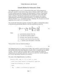
maneuver3.m – finite burn orbit transfer<br />
This MATLAB script simulates a single finite burn maneuver for orbit transfer between two<br />
coplanar elliptical orbits. The user can choose from three types of thrust vector “steering” during<br />
the maneuver. This application assumes a constant thrust level <strong>and</strong> propellant flow rate. The<br />
single finite burn maneuver occurs at the mutual perigee of the initial <strong>and</strong> final orbits, <strong>and</strong> the<br />
burn is “centered” about perigee.<br />
The following is a brief description about each type of steering method.<br />
Tangential<br />
For this type of steering the thrust pointing direction is tangential to the instantaneous radius<br />
vector to the spacecraft <strong>and</strong> in the direction of the orbital motion. This implies that both the<br />
pitch <strong>and</strong> yaw angles are always zero during the finite burn maneuver.<br />
page 8
Gravity turn<br />
<strong>Orbital</strong> <strong>Mechanics</strong> with MATLAB<br />
For this type of steering the thrust pointing direction is always aligned with the instantaneous<br />
velocity vector of the vehicle.<br />
Linear pitch angle<br />
For this third type of steering, the pitch angle of the maneuver changes linearly during the burn.<br />
The angular range over which the maneuver occurs is given by<br />
d 2 t <br />
<br />
where is the orbital period of the initial orbit. The initial <strong>and</strong> final pitch angles of the<br />
maneuver are given by<br />
<br />
i <br />
2<br />
<strong>and</strong><br />
<br />
f <br />
2<br />
The pitch angle at any time t is determined from the following expression<br />
d<br />
dt<br />
t i t tign<br />
<br />
d<br />
where the pitch rate is given by i f / td<br />
<strong>and</strong> tign is the ignition time of the maneuver.<br />
dt<br />
In these expressions td is the thrust duration of the maneuver.<br />
The thrust duration is calculated from the ideal rocket equation with the expression<br />
t<br />
d<br />
gI m<br />
<br />
T<br />
where I sp is the specific impulse <strong>and</strong> m p is the propellant mass required for the maneuver. The<br />
propellant mass is also calculated from the ideal rocket equation.<br />
sp p<br />
The “gravity loss” for a finite burn maneuver is given by:<br />
t<br />
bo<br />
Vg gsin dt<br />
tign<br />
page 9
<strong>Orbital</strong> <strong>Mechanics</strong> with MATLAB<br />
where g is the scalar acceleration of gravity at the location of the maneuver, is the<br />
instantaneous flight path angle, t ign is the ignition time of the maneuver <strong>and</strong> t bo is the burnout or<br />
termination time of the burn. The gravity loss occurs because the g sin term turns the vehicle<br />
away from the optimal thrust direction during a finite burn maneuver.<br />
The inertial delta-velocity added to the vehicle by the finite burn is given by<br />
i<br />
tbo<br />
tign ECI<br />
V T u dt<br />
The total acceleration of the spacecraft is a combination of “Keplerian” gravity <strong>and</strong> thrust<br />
acceleration according to the following expression:<br />
T a g u<br />
m In this equation T is the thrust level, m is the instantaneous mass of the vehicle <strong>and</strong> u ECI is the<br />
inertial unit pointing vector along which the thrust is applied. This script numerically integrates<br />
this system of nonlinear vector differential equations using the rkf78 function while accounting<br />
for the change in spacecraft mass due to propellant expenditure.<br />
The transformation of a unit pointing vector in the radial-tangential-normal (RTN) coordinate<br />
system centered at the spacecraft u RTN to an Earth-centered-inertial (ECI) unit pointing vector<br />
u ECI is given by the following operation:<br />
h r<br />
<br />
h r<br />
page 10<br />
ECI<br />
h r <br />
u h r u<br />
x x x<br />
<br />
ECI hy r y y RTN<br />
<br />
hz r z z<br />
In this matrix h is the angular momentum vector <strong>and</strong> all x, y <strong>and</strong> z components of these matrix<br />
elements are unit vectors.<br />
The RTN unit pointing vector at any mission time t is determined from the pitch <strong>and</strong> yaw angles<br />
as follows:<br />
sintcos t <br />
u RTN t cos t cos<br />
t <br />
sin<br />
t <br />
<br />
For the coplanar case modeled in this MATLAB script, the yaw or out-of-plane angle is<br />
always zero.<br />
The following is a typical user interaction with this script.
<strong>Orbital</strong> <strong>Mechanics</strong> with MATLAB<br />
program maneuver3<br />
< finite burn orbit transfer between elliptical orbits ><br />
initial orbit<br />
please input the perigee altitude (kilometers)<br />
(perigee altitude > 0)<br />
? 300<br />
please input the apogee altitude (kilometers)<br />
(apogee altitude >= perigee altitude)<br />
? 300<br />
final orbit<br />
please input the apogee altitude (kilometers)<br />
(apogee altitude >= perigee altitude)<br />
? 500<br />
please input the thrust (newtons)<br />
(thrust > 0)<br />
? 400<br />
please input the specific impulse (seconds)<br />
(specific impulse > 0)<br />
? 300<br />
please input the initial mass (kilograms)<br />
(initial mass > 0)<br />
? 4000<br />
please select the steering method<br />
? 3<br />
tangential<br />
gravity turn<br />
linear pitch rate<br />
The following is the script output for this example.<br />
program maneuver3<br />
< finite burn orbit transfer between elliptical orbits ><br />
initial orbit<br />
perigee altitude 300.000000 kilometers<br />
apogee altitude 300.000000 kilometers<br />
page 11
<strong>Orbital</strong> <strong>Mechanics</strong> with MATLAB<br />
initial mass 4000.000000 kilograms<br />
thrust 400.000000 newtons<br />
specific impulse 300.000000 seconds<br />
exhaust velocity 2941.995000 meters/seconds<br />
propellant flow rate 0.135962 kilograms/seconds<br />
impulsive maneuver<br />
delta-v 56.781639 meters/second<br />
thrust duration 562.371931 seconds<br />
propellant mass 76.461303 kilograms<br />
finite burn maneuver - linear pitch rate steering<br />
delta-v 56.781626 meters/second<br />
gravity loss 5.778402 meters/second<br />
propellant mass 76.461303 kilograms<br />
pitch rate -0.066284 degrees/second<br />
final orbit<br />
perigee altitude 299.978878 kilometers<br />
apogee altitude 496.473985 kilometers<br />
sma (km) eccentricity inclination (deg) argper (deg)<br />
+6.77636273153397e+003 +1.44985676268658e-002 +0.00000000000000e+000 +5.17362827084665e-002<br />
raan (deg) true anomaly (deg) arglat (deg) period (min)<br />
+0.00000000000000e+000 +1.87112067751264e+001 +1.87629430578349e+001 +9.25240641504207e+001<br />
If this same maneuver was performed with tangential steering, the finite burn <strong>and</strong> final orbit<br />
results are as follows:<br />
finite burn maneuver - tangential steering<br />
delta-v 55.779011 meters/second<br />
gravity loss 7.769443 meters/second<br />
propellant mass 76.461247 kilograms<br />
final orbit<br />
page 12
<strong>Orbital</strong> <strong>Mechanics</strong> with MATLAB<br />
perigee altitude 301.7276 kilometers<br />
apogee altitude 498.2205 kilometers<br />
If this same maneuver was performed with gravity turn steering, the results are as follows:<br />
finite burn maneuver - gravity turn steering<br />
delta-v 55.793099 meters/second<br />
gravity loss 7.783571 meters/second<br />
propellant mass 76.461247 kilograms<br />
final orbit<br />
perigee altitude 301.7154 kilometers<br />
apogee altitude 498.2330 kilometers<br />
ltot.m – low thrust orbit transfer<br />
This MATLAB script determines the characteristics of low-thrust orbital transfer between two<br />
nonplanar circular orbits. The numerical method used in this script is described in Chapter 14 of<br />
the book <strong>Orbital</strong> <strong>Mechanics</strong> by V. Chobotov <strong>and</strong> the technical paper, “The Reformulation of<br />
Edelbaum's Low-thrust Transfer Problem Using Optimal Control Theory” by J. A. Kechichian,<br />
AIAA-92-4576-CP. The original Edelbaum algorithm is described in “Propulsion Requirements<br />
for Controllable Satellites”, ARS Journal, August 1961, pages 1079-1089. This algorithm is<br />
<br />
valid for total inclination changes i given by 0 i114.6 . This algorithm assumes that the<br />
thrust acceleration magnitude <strong>and</strong> spacecraft mass are both constant during the orbit transfer.<br />
The initial thrust vector yaw angle 0 is given by the following expression<br />
sin i<br />
<br />
2<br />
tan 0<br />
<br />
<br />
V0<br />
cos i<br />
<br />
V 2 <br />
f<br />
where the speed on the initial circular orbit is V0 r0<br />
<strong>and</strong> the speed on the final circular<br />
orbit is Vf rf.<br />
In these equations r0 re h0<br />
is the geocentric radius of the initial orbit,<br />
rfre hf<br />
is the geocentric radius of the final orbit, re is the radius of the Earth <strong>and</strong> is the<br />
gravitational constant of the Earth. The initial altitude is h0 <strong>and</strong> the final altitude is hf .<br />
The total velocity change required for a low-thrust orbit transfer is given by<br />
page 13
<strong>Orbital</strong> <strong>Mechanics</strong> with MATLAB<br />
V0sin<br />
0<br />
V V0cos 0<br />
<br />
tan i 0<br />
<br />
2 <br />
The total transfer time is given by t V f where f is the thrust acceleration. The time<br />
evolution of the yaw angle, speed <strong>and</strong> inclination change are given by the following three<br />
expressions:<br />
1 V0sin<br />
0<br />
t tan <br />
V0cos 0<br />
ft<br />
2 2 2<br />
0 2 0 cos0<br />
<br />
V t V V ft f t<br />
2 1<br />
ftV0cos 0 <br />
i t tan <br />
0<br />
V0sin<br />
0<br />
2 <br />
This MATLAB script will prompt you for the initial <strong>and</strong> final altitudes <strong>and</strong> orbital inclinations,<br />
<strong>and</strong> the thrust acceleration. The following is a typical user interaction with this script. It<br />
illustrates an orbital transfer from a low Earth orbit (LEO) with an inclination of 28.5 to a<br />
geosynchronous Earth orbit (GSO) with an orbital inclination of 0. The thrust acceleration for<br />
this example is 3.5E-4 meters/second 2 .<br />
Low-thrust Orbit Transfer Analysis<br />
please input the initial altitude (kilometers)<br />
? 621.86<br />
please input the final altitude (kilometers)<br />
? 35787.86<br />
please input the initial orbital inclination (degrees)<br />
(0
<strong>Orbital</strong> <strong>Mechanics</strong> with MATLAB<br />
initial orbit inclination 28.5000 degrees<br />
initial orbit velocity 7546.0538 meters/second<br />
final orbit altitude 35787.8600 kilometers<br />
final orbit inclination 0.0000 degrees<br />
final orbit velocity 3074.5936 meters/second<br />
total inclination change 28.5000 degrees<br />
total delta-v 5783.7751 meters/second<br />
thrust duration 191.2624 days<br />
initial yaw angle 21.9850 degrees<br />
thrust acceleration 0.000350 meters/second^2<br />
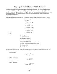
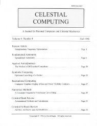
The software will also graphically display the time evolution of the thrust vector yaw angle,<br />
speed, inclination change <strong>and</strong> semimajor axis. The graphics for this example are as follows:<br />
Yaw Angle (deg)<br />
Inclination (deg)<br />
70<br />
60<br />
50<br />
40<br />
30<br />
Low−thrust Orbit Transfer<br />
20<br />
0 20 40 60 80 100 120 140 160 180 200<br />
30<br />
25<br />
20<br />
15<br />
10<br />
5<br />
0<br />
−5<br />
0 20 40 60 80 100 120 140 160 180 200<br />
Simulation Time (days)<br />
page 15
Velocity (m/s)<br />
8000<br />
7000<br />
6000<br />
5000<br />
4000<br />
<strong>Orbital</strong> <strong>Mechanics</strong> with MATLAB<br />
Low−thrust Orbit Transfer<br />
3000<br />
0 20 40 60 80 100 120 140 160 180 200<br />
Semimajor Axis (kilometers)<br />
x 104<br />
5<br />
4<br />
3<br />
2<br />
1<br />
0<br />
0 20 40 60 80 100 120 140 160 180 200<br />
Simulation Time (days)<br />
sep_ltot.m – low-thrust orbit transfer using solar-electric propulsion<br />
This interactive MATLAB script can be used to determine the characteristics of continuous, lowthrust<br />
orbital transfer between two non-coplanar circular orbits using solar-electric propulsion<br />
(SEP). The numerical method used in this script is identical to the technique used in the ltot.m<br />
script described previously.<br />
The propulsive thrust provided by an SEP system is given by<br />
2<br />
P<br />
T <br />
gI<br />
where is the non-dimensional propulsive efficiency, P is the input power in kilowatts, g is the<br />
acceleration of gravity in meters/second <strong>and</strong> I sp is the specific impulse in seconds. The quantity<br />
gI sp is also called the exhaust velocity. Note that with these metric units the thrust will be in<br />
milli-newtons. The thrust acceleration required in the equations to follow is equal to aT T m<br />
where m is the mass of the spacecraft.<br />
This MATLAB script will prompt you for the initial <strong>and</strong> final altitudes <strong>and</strong> orbital inclinations,<br />
<strong>and</strong> the SEP propulsive characteristics. The following is a typical user interaction with this<br />
script. It illustrates an orbital transfer from a low Earth orbit (LEO) with an inclination of 28.5<br />
to a geosynchronous Earth orbit (GSO) with an orbital inclination of 0.<br />
sp<br />
page 16
<strong>Orbital</strong> <strong>Mechanics</strong> with MATLAB<br />
SEP Low-thrust Orbit Transfer Analysis<br />
please input the initial altitude (kilometers)<br />
? 621.86<br />
please input the final altitude (kilometers)<br />
? 35787.86<br />
please input the initial orbital inclination (degrees)<br />
(0
<strong>Orbital</strong> <strong>Mechanics</strong> with MATLAB<br />
final spacecraft mass 959.8933 kilograms<br />
propellant mass 187.8393 kilograms<br />
total inclination change 28.5000 degrees<br />
total delta-v 5783.7751 meters/second<br />
thrust duration 191.2624 days<br />
initial yaw angle 21.9850 degrees<br />
thrust acceleration 0.000350 meters/second^2<br />
The software will also graphically display the time evolution of the thrust vector yaw angle,<br />
spacecraft speed, inclination change <strong>and</strong> semimajor axis.<br />
cdeorbit.m – single impulse de-orbit from a circular orbit<br />
This MATLAB script calculates the single impulsive maneuver required to establish a reentry<br />
altitude <strong>and</strong> flight path angle relative to a non-rotating, spherical Earth. The algorithm uses a<br />
tangential delta-v applied opposite to the velocity vector of an initial circular orbit to establish<br />
the de-orbit trajectory.<br />
The scalar magnitude of the single impulsive maneuver required to de-orbit a spacecraft from an<br />
initial circular orbit can be determined from the following expression<br />
where<br />
<strong>and</strong><br />
V<br />
V<br />
<br />
<br />
1 2r1 2r1 <br />
V Vc 1 V 1<br />
e 2 c <br />
i<br />
2 <br />
r r r<br />
<br />
1 1<br />
cos <br />
e cos<br />
<br />
e <br />
hi req ri<br />
r<br />
radius<br />
ratio<br />
h r r<br />
ce<br />
ci<br />
e eq e<br />
<br />
<br />
r<br />
he req<br />
<br />
<br />
r<br />
hi req<br />
e<br />
i<br />
local circular velocity at entry interface<br />
local circular velocity of initial circular orbit<br />
page 18
h<br />
h<br />
r<br />
<strong>Orbital</strong> <strong>Mechanics</strong> with MATLAB<br />
<br />
e<br />
i<br />
e<br />
r<br />
r<br />
i<br />
e<br />
eq<br />
<br />
<br />
<br />
<br />
<br />
flight path angle at entry interface<br />
altitude of initial circular orbit<br />
altitude at entry interface<br />
radius of initial circular orbit<br />
radius at entry interface<br />
Earth equatorial radius<br />
Earth gravitational constant<br />
This algorithm is described in the technical article, “Deboost from Circular Orbits”, A. H.<br />
Milstead, The Journal of the Astronautical Sciences, Vol. XIII, No. 4, pp. 170-171, Jul-Aug.,<br />
1966. Additional information can be found in Chapter 5 of Hypersonic <strong>and</strong> Planetary Entry<br />
Flight <strong>Mechanics</strong> by Vinh, Busemann <strong>and</strong> Culp, The University of Michigan Press.<br />
The true anomaly on the de-orbit trajectory at the entry interface e can be determined from the<br />
following two equations<br />
2<br />
r<br />
ad 1 ed<br />
sin<br />
e <br />
e <br />
d<br />
2 <br />
ad 1 ed<br />
1<br />
cose<br />
<br />
er e<br />
page 19<br />
d e d<br />
<strong>and</strong> the following four quadrant inverse tangent operation<br />
where<br />
e<br />
a<br />
d<br />
d<br />
<br />
<br />
r<br />
<br />
<br />
<br />
1<br />
e tan sin e,cose eccentricity of the de-orbit trajectory<br />
semimajor axis of the de-orbit trajectory<br />
<br />
2arra1e <br />
2 2 2<br />
d e e<br />
2<br />
ar d e<br />
d d<br />
The elapsed time-of-flight between perigee of the de-orbit trajectory <strong>and</strong> the entry true anomaly<br />
is given by<br />
e<br />
t<br />
e<br />
2<br />
1<br />
1<br />
e<br />
d 1 d sin<br />
d e<br />
e e <br />
e<br />
2tan tan <br />
<br />
2 1ed 2 1ed cos<br />
<br />
e
<strong>Orbital</strong> <strong>Mechanics</strong> with MATLAB<br />
In this equation is the Keplerian orbital period of the de-orbit trajectory <strong>and</strong> is equal to<br />
2 d<br />
3<br />
a .<br />
Therefore, the flight time between the de-orbit impulse <strong>and</strong> entry interface is given by<br />
<br />
t tet180 te 2<br />
Finally, the orbital speed at the entry interface V e can be determined from<br />
V<br />
e<br />
2<br />
<br />
<br />
r a<br />
e d<br />
This MATLAB script will prompt you for the altitude of the initial circular orbit, <strong>and</strong> the entry<br />
altitude <strong>and</strong> flight path angle. The following is a typical user interaction with this script.<br />
program cdeorbit<br />
< single impulse deorbit from circular orbits ><br />
please input the initial altitude (kilometers)<br />
? 1000<br />
please input the entry altitude (kilometers)<br />
? 100<br />
please input the entry flight path angle (degrees)<br />
? -2<br />
The following is the script output created for this example.<br />
program cdeorbit<br />
< single impulse deorbit from circular orbits ><br />
initial altitude 1000.000000 kilometers<br />
entry altitude 100.000000 kilometers<br />
entry fpa -2.000000 degrees<br />
entry trajectory<br />
semimajor axis 6896.07935765 kilometers<br />
eccentricity 0.06990358<br />
page 20
<strong>Orbital</strong> <strong>Mechanics</strong> with MATLAB<br />
argument of perigee 180.00000000 degrees<br />
perigee altitude 35.87871531 kilometers<br />
apogee altitude 1000.00000000 kilometers<br />
entry true anomaly 328.04948058 degrees<br />
entry velocity 8078.31275892 meters/second<br />
impulse-to-entry time 40.13350666 minutes<br />
deorbit delta-v 261.55416617 meters/second<br />
The software will also calculate <strong>and</strong> display the entry velocity <strong>and</strong> flight path angle relative to a<br />
rotating spherical Earth. The following is the relative flight information for this example.<br />
relative flight path coordinates<br />
flight path angle -2.12418719 degrees<br />
velocity magnitude 7.60622497 kilometers/second<br />
Finally, the software will graphically display the initial circular orbit <strong>and</strong> the de-orbit trajectory.<br />
The graphic display for this example is as follows where the red dots represent the original<br />
circular orbit <strong>and</strong> the blue dots represent the de-orbit trajectory, both at one minute intervals.<br />
The black circle is the surface of a spherical Earth <strong>and</strong> the distances are in Earth radii.<br />
y coordinate (Earth radii)<br />
1<br />
0.8<br />
0.6<br />
0.4<br />
0.2<br />
0<br />
−0.2<br />
−0.4<br />
−0.6<br />
−0.8<br />
−1<br />
Single Impulse Deorbit From a Circular Orbit<br />
−1 −0.5 0 0.5 1<br />
x coordinate (Earth radii)<br />
page 21
<strong>Orbital</strong> <strong>Mechanics</strong> with MATLAB<br />
The maneuver creates an elliptical de-orbit trajectory with an apogee located at the maneuver<br />
point. The apogee altitude of this trajectory is equal to the altitude of the initial circular orbit.<br />
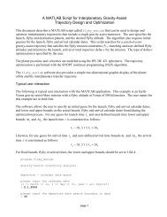
edeorbit.m – single impulse de-orbit from an elliptical orbit<br />
This MATLAB script calculates the single impulsive maneuver required to establish a reentry<br />
altitude <strong>and</strong> flight path angle relative to a non-rotating spherical Earth. The algorithm uses a<br />
tangential V applied opposite to the velocity vector at apogee of the initial elliptical orbit to<br />
establish the de-orbit trajectory that enters the Earth’s atmosphere.<br />
The scalar magnitude of this de-orbit delta-v is given by<br />
where<br />
2r p 2ra1 <br />
V <br />
cos<br />
<br />
2 2<br />
e<br />
r e rara rp rara cos e<br />
<br />
<br />
re<br />
geocentric radius at the entry altitude<br />
ra ra re<br />
rp rp re<br />
e flight path angle at entry<br />
ra<br />
apogee radius of the initial elliptical orbit<br />
rp<br />
perigee radius of the initial elliptical orbit<br />
gravitational<br />
constant of the Earth<br />
The true anomaly at entry can be determined from the following series of equations:<br />
where<br />
e<br />
a<br />
d<br />
d<br />
r<br />
<br />
r<br />
sin<br />
e <br />
e<br />
d<br />
2 <br />
page 22<br />
2 1 <br />
a e<br />
d d<br />
<br />
ad 1 ed<br />
1<br />
cose<br />
<br />
er e<br />
d e d<br />
<br />
<br />
1<br />
e tan sin e,cose eccentricity of deorbit trajectory<br />
semimajor axis of deorbit trajectory<br />
<br />
2arra1e <br />
2 2 2<br />
d e e<br />
2<br />
ar d e<br />
d d
<strong>Orbital</strong> <strong>Mechanics</strong> with MATLAB<br />
<strong>and</strong> the inverse tangent is a four quadrant operation.<br />
The time of flight between perigee <strong>and</strong> the entry true anomaly e is given by:<br />
t<br />
e<br />
2<br />
1<br />
1<br />
e<br />
d 1 d sin<br />
d e<br />
e e <br />
e<br />
2tan tan <br />
<br />
2 1ed 2 1ed cos<br />
<br />
e <br />
In this equation is the orbital period of the de-orbit trajectory.<br />
Therefore, the flight time between the de-orbit impulse time <strong>and</strong> entry is given by<br />
<br />
t tet180 te 2<br />
Finally, the speed at reentry V e can be determined from<br />
V<br />
e<br />
2<br />
<br />
<br />
r a<br />
e d<br />
Please note that these equations are also valid for the case of de-orbit from an initial circular<br />
orbit as described in the previous cdeorbit.m script.<br />
The following is a typical user interaction with this script.<br />
program edeorbit<br />
< single impulse deorbit from elliptical orbits ><br />
please input the perigee altitude (kilometers)<br />
? 285.798<br />
please input the apogee altitude (kilometers)<br />
? 35785.922<br />
please input the entry altitude (kilometers)<br />
? 111.252<br />
please input the entry flight path angle (degrees)<br />
? -4<br />
The following is the script output created for this example.<br />
program edeorbit<br />
< single impulse deorbit from elliptical orbits ><br />
page 23
initial orbit<br />
<strong>Orbital</strong> <strong>Mechanics</strong> with MATLAB<br />
perigee altitude 285.798000 kilometers<br />
apogee altitude 35785.922000 kilometers<br />
semimajor axis 24414.000000 kilometers<br />
eccentricity 0.727044<br />
entry altitude 111.252000 kilometers<br />
entry fpa -4.000000 degrees<br />
entry trajectory<br />
semimajor axis 24308.08290588 kilometers<br />
eccentricity 0.73456961<br />
perigee altitude 73.96381175 kilometers<br />
apogee altitude 35785.92200000 kilometers<br />
entry true anomaly 350.55084585 degrees<br />
entry velocity 10317.40933180 meters/second<br />
entry fpa -4.00000000 degrees<br />
impulse-to-entry time 312.58844372 minutes<br />
deorbit delta-v 22.29796787 meters/second<br />
The software will also calculate <strong>and</strong> display the entry velocity <strong>and</strong> flight path angle relative to a<br />
rotating spherical Earth. The following is the relative flight path information for this example.<br />
relative flight path coordinates<br />
entry velocity 9845.40345708 meters/second<br />
entry fpa -4.19210209 degrees<br />
This MATLAB script will also graphically display the initial elliptic orbit <strong>and</strong> the de-orbit<br />
trajectory.<br />
aeroassist.m – aero-assisted co-planar orbital transfer<br />
This MATLAB script can be used to estimate the propulsive V<br />
required for aero-assisted<br />
coplanar orbital transfer from a high Earth orbit (HEO) to a lower Earth orbit (LEO). Both the<br />
initial <strong>and</strong> final orbits are assumed to be circular. The equations used in this algorithm are<br />
described in “Fuel-Optimal Trajectories for Aeroassisted Coplanar <strong>Orbital</strong> Transfer Problem”,<br />
page 24
<strong>Orbital</strong> <strong>Mechanics</strong> with MATLAB<br />
IEEE Transactions on Aerospace <strong>and</strong> Electronic Systems, Vol. 26, No. 2, March 1990, pg. 374-<br />
380. Another excellent technical discussion can be found in “Minimum-Fuel Aeroassisted<br />
Coplanar Orbit Transfer Using Lift-Modulation”, AIAA Journal of Guidance, Control <strong>and</strong><br />
Dynamics, Vol. 8, No. 1, Jan.-Feb. 1985.<br />
The normalized delta-Vs required to initiate the aeropass, Vd , <strong>and</strong> to re-circularize the orbit<br />
after the aeropass, Vc , are given by<br />
page 25<br />
a <br />
1 21 d<br />
V d <br />
a 2<br />
d a <br />
d<br />
ad<br />
1 2 <br />
cos <br />
entry <br />
a <br />
1 21 c<br />
V c <br />
2<br />
ac a c ac<br />
12 cos <br />
<br />
exit <br />
The normalized speeds at entry into the atmosphere, Ventry , <strong>and</strong> at exit from the atmosphere, Vexit ,<br />
are given by<br />
2ad 1 ad<br />
V<br />
<br />
entry 2 2<br />
cos a<br />
where<br />
V<br />
exit<br />
<br />
entry d<br />
<br />
2a cos<br />
1 a<br />
c c<br />
2 2<br />
exit ac<br />
rd<br />
ad<br />
initial orbit radius ratio<br />
ra<br />
rc<br />
ac<br />
final orbit radius ratio<br />
ra<br />
rd<br />
geocentric radius of the initial orbit<br />
rc<br />
geocentric radius of the final orbit<br />
ra<br />
geocentric radius of the atmosphere<br />
entry flight<br />
path angle at atmospheric entry<br />
exit flight path angle at atmospheric exit<br />
The dimensional speed <strong>and</strong> V can be recovered by multiplying the normalized values by<br />
ra<br />
where is the gravitational constant of the Earth. The quantity a r<br />
circular velocity at the radius of the atmosphere.<br />
is the local
<strong>Orbital</strong> <strong>Mechanics</strong> with MATLAB<br />
The following is a typical user interaction with this script.<br />
program aeroassist<br />
< aeroassisted orbit transfer between circular orbits ><br />
please input the initial altitude (kilometers)<br />
? 35786<br />
please input the final altitude (kilometers)<br />
? 300<br />
please input the entry altitude (kilometers)<br />
? 120<br />
please input the entry flight path angle (degrees)<br />
? -3<br />
please input the exit flight path angle (degrees)<br />
? 1<br />
The following is the script output for this example.<br />
aeroassist orbit transfer<br />
initial altitude 35786.0000 kilometers<br />
final altitude 300.0000 kilometers<br />
entry flight path angle -3.0000 degrees<br />
entry speed 10309.8017 meters/second<br />
exit flight path angle 1.0000 degrees<br />
exit speed 7864.0519 meters/second<br />
deorbit delta-v 1487.9405 meters/second<br />
circularization delta-v 74.8372 meters/second<br />
total delta-v 1562.7777 meters/second<br />
For comparison purposes the software will also display the all-propulsive Hohmann orbit transfer<br />
for this example.<br />
Hohmann orbit transfer<br />
deorbit delta-v 1466.8241 meters/second<br />
circularization delta-v 2425.7315 meters/second<br />
total delta-v 3892.5557 meters/second<br />
page 26
<strong>Orbital</strong> <strong>Mechanics</strong> with MATLAB<br />
The aeroassist Matlab script will also create parametric graphic displays of several important<br />
flight parameters. In addition to the screen displays, the script will create color eps disk files of<br />
these plots using source code similar to print -depsc -tiff -r300 aeroassist3.eps.<br />
The following is a plot of the entry speed <strong>and</strong> de-orbit delta-v as a function of the flight path<br />
angle at entry into the Earth’s atmosphere.<br />
entry speed (km/s)<br />
deorbit delta−v (km/s)<br />
10.31<br />
10.3098<br />
10.3096<br />
10.3094<br />
10.3092<br />
Aeroassist Orbit Transfer<br />
10.309<br />
−5 −4.5 −4 −3.5 −3 −2.5 −2<br />
1.493<br />
1.492<br />
1.491<br />
1.49<br />
1.489<br />
1.488<br />
1.487<br />
1.486<br />
−5 −4.5 −4 −3.5 −3 −2.5 −2<br />
entry flight path angle (degrees)<br />
The following is a plot of the exit speed <strong>and</strong> circularization delta-v as a function of the flight path<br />
angle at exit from the atmosphere.<br />
exit speed (km/s)<br />
reorbit delta−v (km/s)<br />
7.9<br />
7.85<br />
7.8<br />
7.75<br />
7.7<br />
7.65<br />
7.6<br />
Aeroassist Orbit Transfer<br />
7.55<br />
0 0.5 1 1.5 2 2.5 3 3.5 4<br />
0.4<br />
0.35<br />
0.3<br />
0.25<br />
0.2<br />
0.15<br />
0.1<br />
0.05<br />
0 0.5 1 1.5 2 2.5 3 3.5 4<br />
exit flight path angle (degrees)<br />
page 27
<strong>Orbital</strong> <strong>Mechanics</strong> with MATLAB<br />
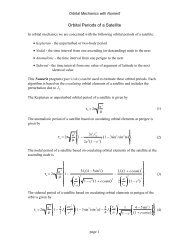
The final plot created by this script illustrates the combinations of initial <strong>and</strong> final orbit radii<br />
where the orbit transfer is performed more efficiently using total propulsive (Hohmann)<br />
maneuvers versus aeroassisted maneuvers.<br />
The following is the plot for this example. It uses the atmospheric altitude, entry flight path<br />
angle <strong>and</strong> exit flight path angle provided by the user. In this plot r i is the radius of the initial<br />
circular orbit, f r the radius of the final circular orbit, <strong>and</strong> r a the radius of the atmosphere.<br />
r f / r a<br />
2.1<br />
2<br />
1.9<br />
1.8<br />
1.7<br />
1.6<br />
1.5<br />
1.4<br />
1.3<br />
1.2<br />
Hohmann Transfer<br />
The Hohmann Orbit Transfer<br />
Aeroassist Orbit Transfer<br />
1.1<br />
1 2 3 4 5<br />
r / r<br />
i a<br />
6 7 8 9<br />
page 28<br />
Aeroassist Transfer<br />
This section summarizes the equations that define the Hohmann orbit transfer <strong>and</strong> describes a<br />
MATLAB script that solves this classic astrodynamic problem. The software can solve both the<br />
coplanar <strong>and</strong> non-coplanar orbit transfer problem.<br />
hohmann.m – Hohmann two impulse orbital transfer<br />
The coplanar circular orbit-to-circular orbit transfer was discovered by the German engineer<br />
Walter Hohmann in 1925 <strong>and</strong> described in his classic report, The Attainability of <strong>Celestial</strong><br />
Bodies. The transfer consists of a velocity impulse on an initial circular orbit, in the direction of<br />
motion <strong>and</strong> collinear with the velocity vector, which propels the space vehicle into an elliptical<br />
transfer orbit. At a transfer angle of 180 degrees from the first impulse, a second velocity<br />
impulse or V , also collinear <strong>and</strong> in the direction of motion, places the vehicle into a final<br />
circular orbit at the desired final altitude. The impulsive V assumption means that the velocity,<br />
but not the position, of the vehicle is changed instantaneously. This is equivalent to a rocket<br />
engine with infinite thrust magnitude. Therefore, the Hohmann formulation is the ideal <strong>and</strong><br />
minimum energy solution to this type of orbit transfer problem.
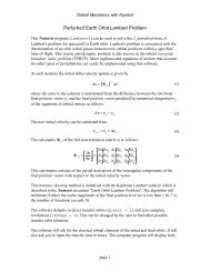
Coplanar Equations<br />
<strong>Orbital</strong> <strong>Mechanics</strong> with MATLAB<br />
For the coplanar Hohmann transfer both velocity impulses are confined to the orbital planes of<br />
the initial <strong>and</strong> final orbits. The first impulse creates an elliptical transfer orbit with a perigee<br />
altitude equal to the altitude of the initial circular orbit <strong>and</strong> an apogee altitude equal to the<br />
altitude of the final orbit. The second impulse circularizes the transfer orbit at apogee. Both<br />
impulses are posigrade which means that they are in the direction of orbital motion.<br />
We begin by defining three normalized radii as follows:<br />
R<br />
R<br />
R<br />
1<br />
2<br />
3<br />
<br />
<br />
<br />
rf<br />
2<br />
r r<br />
ri<br />
r<br />
f<br />
ri<br />
2<br />
r r<br />
where ri is the geocentric radius of the initial circular park orbit <strong>and</strong> rf is the radius of the final<br />
circular mission orbit. The relationship between radius <strong>and</strong> initial orbit altitude hi <strong>and</strong> the final<br />
orbit altitude hf is as follows:<br />
r r h<br />
where r e is the radius of the Earth.<br />
The magnitude of the first impulse is<br />
page 29<br />
i f<br />
i f<br />
i e i<br />
r r h<br />
f e f<br />
V V 1R 2R<br />
1 lc<br />
2<br />
1 1<br />
<strong>and</strong> is simply the difference between the speed on the initial orbit <strong>and</strong> the perigee speed of the<br />
transfer orbit. The scalar magnitude of the second impulse is<br />
V V R R R 2R<br />
R<br />
2 2 2 2<br />
2 lc 2 2 3 2 3<br />
which is the difference between the speed on the final orbit <strong>and</strong> the apogee speed of the transfer<br />
ellipse. In each of these V equations Vlc is called the local circular velocity. It can be<br />
determined from<br />
<br />
Vlc<br />
<br />
r<br />
<strong>and</strong> represents the scalar speed in the initial orbit. In these equations is the gravitational<br />
i
<strong>Orbital</strong> <strong>Mechanics</strong> with MATLAB<br />
constant of the central body. The transfer time from the first impulse to the second is equal to<br />
one half the orbital period of the transfer ellipse<br />
3<br />
a<br />
<br />
<br />
where a is the semimajor axis of the transfer orbit <strong>and</strong> is equal to ri rf<br />
/2.<br />
The orbital<br />
eccentricity of the transfer ellipse is<br />
ri rf ri rf<br />
<br />
max , min ,<br />
e <br />
r r<br />
f i<br />
The following diagram illustrates the geometry of the coplanar Hohmann transfer.<br />
Non-coplanar Equations<br />
V 2<br />
r i<br />
final orbit<br />
transfer orbit<br />
page 30<br />
V 1<br />
initial orbit<br />
The non-coplanar Hohmann transfer involves orbital transfer between two circular orbits which<br />
have different orbital inclinations. For this problem the propulsive energy is minimized if we<br />
optimally partition the total orbital inclination change between the first <strong>and</strong> second impulses.<br />
The scalar magnitude of the first impulse is<br />
V V 1R 2R cos<br />
1 lc<br />
2<br />
1 1 1<br />
where 1 is the plane change associated with the first impulse. The magnitude of the second<br />
impulse is<br />
2 2 2 2<br />
V2 Vlc R2 R2R3 <br />
2R2R3cos2 r f
<strong>Orbital</strong> <strong>Mechanics</strong> with MATLAB<br />
where 2 is the plane change associated with the second impulse. These two equations are<br />
different forms of the law of cosines.<br />
The total V required for the maneuver is the sum of the two impulses as follows<br />
V V1 V2<br />
The relationship between the plane change angles is<br />
<br />
t<br />
1 2<br />
where t is the total plane change angle between the initial <strong>and</strong> final orbits.<br />
Optimizing the non-coplanar Hohmann transfer involves allocating the total plane change angle<br />
between the two maneuvers such that the total V required for the mission is minimized. We<br />
can determine this answer by solving for the root of a derivative.<br />
The partial derivative of the total V with respect to the first plane change angle is given by:<br />
page 31<br />
sintcos costsin <br />
<br />
V R<br />
RR<br />
<br />
<br />
1sin1 2<br />
2 3 1 1<br />
1 1<br />
2<br />
R1 2R1cos 1<br />
2<br />
R2 2 2<br />
R2R3 2<br />
2R2R3cos t 1<br />
If we determine the value of 1 which makes this derivative zero, we have found the optimum<br />
plane change required at the first impulse. Once 1 is calculated we can determine 2 from the<br />
total plane change angle relationship <strong>and</strong> the velocity impulses from the previous equations.<br />
Numerical Solution<br />
This numerical algorithm has been implemented in an interactive MATLAB script called<br />
hohmann.m. This script prompts the user for the initial <strong>and</strong> final altitudes in kilometers <strong>and</strong> the<br />
initial <strong>and</strong> final orbital inclinations in degrees. The software then calls the Brent root-finding<br />
algorithm to solve the partial derivative equation described above.<br />
The call to the Brent root-finding algorithm is as follows:<br />
[xroot, froot] = brent('hohmfunc', 0, dinc, rtol)<br />
where hohmfunc is the objective function for this problem. Since we know that the optimum<br />
first plane change angle is somewhere between 0 <strong>and</strong> the total plane change angle dinc, we pass<br />
these as the bounds of the root. In the parameter list rtol is the user-defined root-finding<br />
convergence tolerance.<br />
This is a typical orbit transfer from a low altitude Earth orbit (LEO) at an altitude of 185.2<br />
kilometers <strong>and</strong> an orbital inclination of 28.5 degrees to a geosynchronous Earth orbit (GEO) at<br />
an altitude of 35786.36 kilometers <strong>and</strong> 0 degrees inclination.
<strong>Orbital</strong> <strong>Mechanics</strong> with MATLAB<br />
The following is a V diagram for the first maneuver of this orbit transfer example. In this view<br />
we are looking along the line of nodes which is the mutual intersection of the park <strong>and</strong> transfer<br />
orbit planes with the equatorial plane.<br />
<br />
page 32<br />
<br />
<br />
<br />
<br />
In this diagram Vi is the speed on the initial park orbit, Vp is the perigee speed of the elliptic<br />
transfer orbit, <strong>and</strong> V is the V required for the first maneuver. The inclinations of the park<br />
<strong>and</strong> transfer orbit are also labeled. From this geometry <strong>and</strong> the law of cosines, the required V<br />
is given by<br />
2 2<br />
V V V 2VV cos<br />
i<br />
i p i p<br />
where i is the inclination difference or plane change between the park <strong>and</strong> transfer orbits.<br />
The following is a typical user interaction with this script.<br />
Hohmann Orbit Transfer Analysis<br />
please input the initial altitude kilometers<br />
? 300<br />
please input the final altitude kilometers<br />
? 35786.2<br />
please input the initial orbital inclination degrees<br />
(0
<strong>Orbital</strong> <strong>Mechanics</strong> with MATLAB<br />
initial orbit inclination 28.5000 degrees<br />
initial orbit velocity 7725.7606 meters/second<br />
final orbit altitude 35786.2000 kilometers<br />
final orbit inclination 0.0000 degrees<br />
final orbit velocity 3074.6540 meters/second<br />
first inclination change 2.2002 degrees<br />
second inclination change 26.2998 degrees<br />
total inclination change 28.5000 degrees<br />
first delta-v 2449.4551 meters/second<br />
second delta-v 1781.8532 meters/second<br />
total delta-v 4231.3083 meters/second<br />
transfer orbit eccentricity 0.72654389<br />
transfer orbit perigee velocity 10151.4962 meters/second<br />
transfer orbit apogee velocity 1607.8298 meters/second<br />
Primer Vector Analysis<br />
This section describes a MATLAB script named primer.m that demonstrates how to use primer<br />
vector theory to analyze the performance of impulsive orbital transfers. The term primer vector<br />
was invented by Derek F. Lawden <strong>and</strong> represents the adjoint vector for velocity. A technical<br />
discussion about primer theory can be found in Lawden’s classic text, Optimal Trajectories for<br />
Space Navigation, Butterworths, London, 1963. Another excellent resource is “Primer Vector<br />
Theory <strong>and</strong> Applications”, Donald J. Jezewski, NASA TR R-454, November 1975, along with<br />
“Optimal, Multi-burn, Space Trajectories”, also by Jezewski.<br />
As shown by Lawden, the following four necessary conditions must be satisfied in order for an<br />
impulsive orbital transfer to be locally optimal:<br />
(1) the primer vector <strong>and</strong> its first derivative are everywhere continuous<br />
(2) whenever a velocity impulse occurs, the primer is a unit vector aligned with the impulse<br />
ppˆuˆ<strong>and</strong> p 1<br />
<strong>and</strong> has unit magnitude T <br />
(3) the magnitude of the primer vector may not exceed unity on a coasting arc p<br />
p 1<br />
page 33
<strong>Orbital</strong> <strong>Mechanics</strong> with MATLAB<br />
(4) at all interior impulses (not at the initial or final times) pp 0 ; therefore, d p dt 0<br />
at the intermediate impulses<br />
Furthermore, the scalar magnitudes of the primer vector derivative at the initial <strong>and</strong> final<br />
impulses provide information about how to improve the nominal transfer trajectory by changing<br />
the endpoint times <strong>and</strong>/or moving the impulse times. These four cases for non-zero slopes are<br />
summarized as follows;<br />
If p 0 0 <strong>and</strong> p f 0 perform an initial coast before the first impulse <strong>and</strong> add a final<br />
coast after the second impulse<br />
If p 0 0 <strong>and</strong> p f 0 perform an initial coast before the first impulse <strong>and</strong> move the<br />
second impulse to a later time<br />
If p 0 0 <strong>and</strong> p f 0 perform the first impulse at an earlier time <strong>and</strong> add a final coast<br />
after the second impulse<br />
If p 0 0 <strong>and</strong> p f 0 perform the first impulse at an earlier time <strong>and</strong> move the second<br />
impulse to a later time<br />
The primer vector analysis of a two impulse orbital transfer involves the following steps.<br />
First partition the two-body state transition matrix as follows:<br />
where<br />
<strong>and</strong> so forth.<br />
tt , <br />
r r<br />
<br />
r v <br />
<br />
<br />
0 0 11 12 rr rv<br />
0 <br />
v v<br />
21 22<br />
vr vv<br />
<br />
r0 v0<br />
x / x0 x/ y0 x/ z0<br />
r 11 <br />
<br />
y/ x0 y/ y0 y/ z<br />
<br />
<br />
0<br />
r0 z/ x0 z/ y0 z/ z0<br />
The value of the primer vector at any time t along a two body trajectory is given by<br />
<strong>and</strong> the value of the primer vector derivative is<br />
t t, t t, t <br />
p p p<br />
11 0 0 12 0 0<br />
t t, t t, t <br />
p p p<br />
21 0 0 22 0 0<br />
page 34
which can also be expressed as<br />
<strong>Orbital</strong> <strong>Mechanics</strong> with MATLAB<br />
0 <br />
tt , 0 <br />
0<br />
p<br />
p<br />
<br />
p p <br />
The primer vector boundary conditions at the initial <strong>and</strong> final impulses are as follows:<br />
V<br />
V<br />
0<br />
f<br />
pt0p0 ptf p<br />
f <br />
V V<br />
0<br />
These two conditions illustrate that at the locations of velocity impulses, the primer vector is a<br />
unit vector in the direction of the impulse.<br />
The value of the primer vector derivative at the initial time is<br />
1<br />
t tf, t f tf, t <br />
page 35<br />
<br />
p p p p<br />
0 0 12 0 11 0 0<br />
provided the 12 sub-matrix is non-singular. The value of the primer vector derivative at the<br />
final time is<br />
1<br />
p tf p f 21 tf, t0p022 tf, t012 tf, t0p f 11<br />
tf, t0p0<br />
<br />
f<br />
<br />
The scalar magnitude of the derivative of the primer vector can be determined from<br />
2<br />
d p d pp <br />
pp <br />
dt dt p<br />
The primer.m MATLAB script creates plots of the scalar magnitudes of the primer vector <strong>and</strong><br />
its derivative for a two impulse, coplanar Hohmann transfer. It will request the altitudes of the<br />
initial <strong>and</strong> final circular orbits.<br />
The following is a typical user interaction with this script.<br />
Primer Vector Analysis<br />
please input the initial altitude (kilometers)<br />
? 185.2<br />
please input the final altitude (kilometers)<br />
? 35786<br />
An example of the output produced by this application is<br />
Primer Vector Analysis
<strong>Orbital</strong> <strong>Mechanics</strong> with MATLAB<br />
initial orbit altitude 185.2000 kilometers<br />
initial orbit inclination 0.0000 degrees<br />
initial orbit velocity 7793.0337 meters/second<br />
final orbit altitude 35786.0000 kilometers<br />
final orbit inclination 0.0000 degrees<br />
final orbit velocity 3074.6613 meters/second<br />
first delta-v 2458.9100 meters/second<br />
second delta-v 1478.8275 meters/second<br />
total delta-v 3937.7375 meters/second<br />
transfer orbit eccentricity 0.73061044<br />
transfer orbit perigee velocity 10251.9438 meters/second<br />
transfer orbit apogee velocity 1595.8338 meters/second<br />
transfer time-of-flight 18923.2978 seconds<br />
The following are plots of the scalar magnitude of the primer vector <strong>and</strong> primer derivative as a<br />
function of elapsed trajectory time for this coplanar orbital transfer. From these plots <strong>and</strong> the<br />
necessary conditions for optimality, we can see that this is a locally optimal two impulse transfer<br />
trajectory since p0 p 1.<br />
primer vector magnitude<br />
1<br />
0.95<br />
0.9<br />
0.85<br />
0.8<br />
0 0.2 0.4 0.6 0.8 1 1.2 1.4 1.6 1.8 2<br />
x 10 4<br />
0.75<br />
simulation time (seconds)<br />
f<br />
Primer Vector Analysis<br />
From this plot of the primer derivative magnitude p0pf0 primer derivative magnitude<br />
2<br />
0<br />
−2<br />
−4<br />
−6<br />
−8<br />
−10<br />
−12<br />
−14<br />
page 36<br />
x 10−5<br />
4<br />
Primer Vector Analysis<br />
0 0.2 0.4 0.6 0.8 1 1.2 1.4 1.6 1.8 2<br />
x 10 4<br />
−16<br />
simulation time (seconds)<br />
<strong>and</strong> the rules for moving<br />
impulses or adding coasts, no modifications of this trajectory will reduce the total delta-v.
Phasing Analysis<br />
<strong>Orbital</strong> <strong>Mechanics</strong> with MATLAB<br />
This section describes a MATLAB script called phasing.m that performs a phasing or<br />
rendezvous analysis accomplished with a two impulse, coplanar Hohmann transfer. This script<br />
computes <strong>and</strong> displays a complete analysis of the phasing maneuvers along with a graphics<br />
display of the initial orbit <strong>and</strong> final orbits, the transfer trajectory <strong>and</strong> the orbital locations of the<br />
spacecraft <strong>and</strong> maneuvers.<br />
In this script, the spacecraft on the inner circular orbit is called the chaser <strong>and</strong> the spacecraft on<br />
the outer circular orbit is called the target.<br />
The phasing.m script will prompt the user for the altitudes of the initial <strong>and</strong> final circular<br />
orbits, the initial true anomaly of the chaser vehicle <strong>and</strong> the initial lead angle of the target vehicle<br />
relative to the chaser. This initial lead angle can be either the “ideal” Hohmann value computed<br />
by the script or a user-defined value.<br />
The following a typical interaction with this script.<br />
TWO IMPULSE PHASING ANALYSIS<br />
please input the initial altitude (kilometers)<br />
? 500<br />
please input the true anomaly on the initial orbit (degrees)<br />
(0
chaser initial conditions<br />
-------------------------<br />
altitude 500.000000 kilometers<br />
<strong>Orbital</strong> <strong>Mechanics</strong> with MATLAB<br />
sma (km) eccentricity inclination (deg) argper (deg)<br />
+6.87813630000000e+003 +0.00000000000000e+000 +0.00000000000000e+000 +0.00000000000000e+000<br />
raan (deg) true anomaly (deg) arglat (deg) period (min)<br />
+0.00000000000000e+000 +4.50000000000000e+001 +4.50000000000000e+001 +9.46162866922553e+001<br />
rx (km) ry (km) rz (km) rmag (km)<br />
+4.86357681965535e+003 +4.86357681965535e+003 +0.00000000000000e+000 +6.87813630000000e+003<br />
vx (kps) vy (kps) vz (kps) vmag (kps)<br />
-5.38292709812771e+000 +5.38292709812772e+000 +0.00000000000000e+000 +7.61260850743786e+000<br />
target initial conditions<br />
-------------------------<br />
altitude 5000.000000 kilometers<br />
sma (km) eccentricity inclination (deg) argper (deg)<br />
+1.13781363000000e+004 +0.00000000000000e+000 +0.00000000000000e+000 +0.00000000000000e+000<br />
raan (deg) true anomaly (deg) arglat (deg) period (min)<br />
+0.00000000000000e+000 +9.00000000000000e+001 +9.00000000000000e+001 +2.01310501632031e+002<br />
rx (km) ry (km) rz (km) rmag (km)<br />
+6.96709910002865e-013 +1.13781363000000e+004 +0.00000000000000e+000 +1.13781363000000e+004<br />
vx (kps) vy (kps) vz (kps) vmag (kps)<br />
-5.91879528089421e+000 +3.62421684777778e-016 +0.00000000000000e+000 +5.91879528089421e+000<br />
transfer orbit initial conditions<br />
---------------------------------<br />
sma (km) eccentricity inclination (deg) argper (deg)<br />
+9.12813630000000e+003 +2.46490622625782e-001 +0.00000000000000e+000 +3.53571678494045e+002<br />
raan (deg) true anomaly (deg) arglat (deg) period (min)<br />
+0.00000000000000e+000 +0.00000000000000e+000 +3.53571678494045e+002 +1.44654819447959e+002<br />
rx (km) ry (km) rz (km) rmag (km)<br />
+6.83489138174017e+003 -7.70077113795533e+002 +0.00000000000000e+000 +6.87813630000000e+003<br />
vx (kps) vy (kps) vz (kps) vmag (kps)<br />
+9.51571536023532e-001 +8.44576208559208e+000 +0.00000000000000e+000 +8.49919911489282e+000<br />
trajectory times<br />
----------------<br />
transfer time-of-flight 4339.644583 seconds<br />
72.327410 minutes<br />
wait time 10542.961601 seconds<br />
175.716027 minutes<br />
total mission time 14882.606185 seconds<br />
248.043436 minutes<br />
page 38
conditions at first impulse<br />
---------------------------<br />
<strong>Orbital</strong> <strong>Mechanics</strong> with MATLAB<br />
chaser true anomaly 353.571678 degrees<br />
target true anomaly 44.229854 degrees<br />
transfer orbit true anomaly 0.000000 degrees<br />
conditions at second impulse<br />
----------------------------<br />
chaser true anomaly 268.766028 degrees<br />
target true anomaly 173.571678 degrees<br />
transfer orbit true anomaly 180.000000 degrees<br />
maneuver summary<br />
----------------<br />
first delta-vx 99.262810 meters/second<br />
first delta-vy 881.016345 meters/second<br />
first delta-vz 0.000000 meters/second<br />
first deltav-magnitude 886.590607 meters/second<br />
second delta-vx -87.439739 meters/second<br />
second delta-vy -776.079577 meters/second<br />
second delta-vz 0.000000 meters/second<br />
second deltav-magnitude 780.989896 meters/second<br />
total delta-v 1667.580503 meters/second<br />
The following is the graphics output for this example. In this plot, the red circle is the surface of<br />
the spherical Earth, the green circle is the initial orbit <strong>and</strong> the blue circle is the final orbit. The<br />
black trace is the transfer trajectory at 60 second intervals. The small green circle is the initial<br />
location of the chaser vehicle <strong>and</strong> the small blue square is the initial location of the target<br />
vehicle.<br />
The small black square is the location of the target vehicle at the time of the first impulse <strong>and</strong> the<br />
small black circle is the location of the chaser vehicle at the time of the second impulse. The two<br />
black asterisks are the locations of the two velocity impulses. They are also the locations of the<br />
chaser <strong>and</strong> target vehicles at the maneuver times.<br />
page 39
y−component (ER)<br />
1.5<br />
1<br />
0.5<br />
0<br />
−0.5<br />
−1<br />
−1.5<br />
<strong>Orbital</strong> <strong>Mechanics</strong> with MATLAB<br />
Two Impulse Phasing Analysis<br />
−2 −1.5 −1 −0.5 0 0.5 1 1.5 2<br />
x−component (ER)<br />
This script also performs a graphical primer vector analysis of the transfer trajectory. Please see<br />
the discussion in the previous Primer Vector Analysis section for information about this feature.<br />
Here are the plots of the primer vector <strong>and</strong> its derivative for this example.<br />
primer vector magnitude<br />
1.005<br />
1<br />
0.995<br />
0.99<br />
0.985<br />
0.98<br />
Primer Vector Analysis<br />
0.975<br />
0 500 1000 1500 2000 2500 3000 3500 4000 4500<br />
simulation time (seconds)<br />
primer derivative magnitude<br />
1<br />
0.5<br />
0<br />
−0.5<br />
−1<br />
−1.5<br />
−2<br />
page 40<br />
x 10−5<br />
1.5<br />
Primer Vector Analysis<br />
−2.5<br />
0 500 1000 1500 2000 2500 3000 3500 4000 4500<br />
simulation time (seconds)<br />
The “ideal” Hohmann lead angle is the lead angle the target vehicle must have relative to the<br />
chaser vehicle in order for the 180 transfer to intercept the target. It can be computed from<br />
32<br />
1 1 2 <br />
<br />
H R<br />
R
where<br />
<strong>Orbital</strong> <strong>Mechanics</strong> with MATLAB<br />
Rr1 r2<br />
r1<br />
radius of the chaser circular orbit<br />
r radius of the target circular orbit<br />
2<br />
If the initial lead angle is not equal to the “ideal” Hohmann value, a waiting time is required<br />
before the first impulsive maneuver can be performed. This wait time is given by<br />
where<br />
twait<br />
<br />
s <br />
2<br />
H<br />
user-defined initial lead angle<br />
synodic period of chaser/target orbits<br />
s<br />
The synodic period is computed from the orbital periods of the chaser <strong>and</strong> target orbits using the<br />
following equation;<br />
12 s <br />
<br />
2 1<br />
In this expression, 1 is the orbital period of the chaser vehicle <strong>and</strong> 2 is the orbital period of the<br />
target vehicle. The orbital period can be computed from the circular orbit radius r according to<br />
3<br />
2 r <br />
where is the gravitational constant of the central body.<br />
The equations for computing the impulsive delta-v vectors <strong>and</strong> magnitudes can be found in the<br />
Hohmann transfer discussion given earlier in this document.<br />
Two good resources for this material are “Optimal Multiple-Impulse Time-Fixed Rendezvous<br />
Between Circular Orbits”, John E. Prussing <strong>and</strong> Jeng-Hua Chiu, AIAA Journal of Guidance <strong>and</strong><br />
Control, Vol. 9, No. 1, January-February 1986, pp. 17-22, <strong>and</strong> “Transfer Between Vehicles in<br />
Circular Orbits”, Bernard H. Paiewonsky, Jet Propulsion, February 1958, pp.121-123.<br />
page 41