Emmanuel Amiot Modèles algébriques et algorithmes pour la ...
Emmanuel Amiot Modèles algébriques et algorithmes pour la ...
Emmanuel Amiot Modèles algébriques et algorithmes pour la ...

You also want an ePaper? Increase the reach of your titles
YUMPU automatically turns print PDFs into web optimized ePapers that Google loves.
Thèse de Doctorat de l'Université Pierre <strong>et</strong> Marie Curie<br />
EDITE<br />
Présentée par<br />
<strong>Emmanuel</strong> <strong>Amiot</strong><br />
Pour obtenir le grade de<br />
Docteur de l'Université Pierre <strong>et</strong> Marie Curie<br />
<strong>Modèles</strong> <strong>algébriques</strong> <strong>et</strong> <strong>algorithmes</strong> <strong>pour</strong><br />
<strong>la</strong> formalisation mathématique de structures musicales<br />
Soutenue le 5 mai 2010<br />
devant le jury, composé de<br />
M. Carlos Agon, directeur de thèse<br />
M. Moreno Andreatta, co-directeur<br />
M. David C<strong>la</strong>mpitt, rapporteur<br />
M. Jean-Paul Allouche, rapporteur<br />
M. Thomas Noll, examinateur.<br />
M. <strong>Emmanuel</strong> Saint-James, examinateur<br />
Université Pierre & Marie Curie — Paris 6<br />
Bureau d’accueil, inscription des doctorants <strong>et</strong> base de données<br />
Esc G, 2 ème étage<br />
15 rue de l’école de médecine<br />
75270-PARIS CEDEX 06 Tél. Secrétariat : 01 42 34 68 35<br />
Fax : 01 42 34 68 40<br />
Tél. <strong>pour</strong> les étudiants de A à EL : 01 42 34 69 54<br />
Tél. <strong>pour</strong> les étudiants de EM à MON : 01 42 34 68 41<br />
Tél. <strong>pour</strong> les étudiants de MOO à Z : 01 42 34 68 51<br />
E-mail : sco<strong>la</strong>rite.doctorat@upmc.fr<br />
p. 1
p. 2
Résumé :<br />
C<strong>et</strong>te thèse sur travaux est fondée sur cinq articles, sélectionnés tant <strong>pour</strong> leur inté-<br />
rêt que <strong>pour</strong> leur représentativité. La synthèse ci-jointe vise à rep<strong>la</strong>cer <strong>et</strong> à expliciter le rôle de<br />
ces travaux dans le contexte de <strong>la</strong> recherche contemporaine en Mathématiques <strong>et</strong> Musique. L'<br />
auteur a été amené à utiliser des outils <strong>algébriques</strong> é<strong>la</strong>borés afin de mieux modéliser trois pro-<br />
blèmes d'origine musicale: les canons rythmiques, les gammes, <strong>et</strong> les mélodies autosimi<strong>la</strong>ires.<br />
Sa démarche s'avère ainsi indissociable des sciences de l'informatique, sous leur double fac<strong>et</strong>te<br />
d'expérimentation <strong>et</strong> d'implémentation de logiciels dédiés à l'analyse <strong>et</strong> à <strong>la</strong> composition musi-<br />
cale.<br />
Mots clefs :<br />
Mathémusique, pavage, mosaïque, canons rythmiques, conjecture spectrale, Fugle-<br />
de, canons de Vuza, gammes, Maximally Even S<strong>et</strong>s, transformée de Fourier discrète, tempéra-<br />
ments, autosimi<strong>la</strong>rité, mélodies, affine, modu<strong>la</strong>ire.<br />
p. 3
English title:<br />
Algebraic models and algorithms for the mathematical formali-<br />
Abstract:<br />
zation of musical structures.<br />
This PhD is based on a selection of five previously published papers. They have<br />
been singled out for their scientific interest. The synthesis document aims at making clear the<br />
role and purpose of these papers in the field of contemporary research across mathematics and<br />
music. Their author makes use of sophisticated algebraic notions the b<strong>et</strong>ter to study three<br />
main topics of musical lineage: rhythmic canons, musical scales, and autosimi<strong>la</strong>r melodies. His<br />
approach intertwines with information sciences, on the one hand as a means of experimenta-<br />
tion and on the other hand in producing software for musical analysis and composition.<br />
Keywords:<br />
Mathematics, music, tiling, mosaic, rythmiques canons, spectral conjecture, Fugle-<br />
de, Vuza canons, musical scales, Maximally Even S<strong>et</strong>s, discr<strong>et</strong>e Fourier transform, tempera-<br />
ments, tuning, autosimi<strong>la</strong>rity, melody, affine, modu<strong>la</strong>r.<br />
p. 4
Table des matières<br />
Introduction 6<br />
Bref historique 6<br />
Mes différents champs de recherche 8<br />
Produits de mes recherches 14<br />
Canons rythmiques 14<br />
Gammes <strong>et</strong> transformée de Fourier discrète 22<br />
Mélodies Autosimi<strong>la</strong>ires 30<br />
Conclusion <strong>et</strong> perspectives 37<br />
Remerciements 42<br />
Liste de travaux 45<br />
p. 5
Bref historique<br />
Introduction<br />
Avant de présenter ma recherche, il me semble important de r<strong>et</strong>racer le parcours<br />
intellectuel <strong>et</strong> personnel qui m'y a conduit.<br />
Le cursus traditionnel de mes études (ENS, agrégation) me prédisposait naturelle-<br />
ment à des recherches en mathématiques «pures». Cependant, mes incursions dans ces domai-<br />
nes (j’ai suivi un DEA sur les groupes <strong>et</strong> algèbres de Lie à l'université de Jussieu en 1983) m’ont<br />
convaincu que je ne m'y épanouirai pas. En particulier, ma passion <strong>pour</strong> <strong>la</strong> musique 1, structurée<br />
par mon cursus au Conservatoire de Nice, n'y trouvait pas sa p<strong>la</strong>ce.<br />
C’est en rencontrant André Riotte, compositeur, ingénieur <strong>et</strong> enseignant novateur à<br />
Paris VIII d’un module intitulé Informatique <strong>et</strong> structures musicales, que j’ai trouvé ma voie. La<br />
formalisation mathématique de structures musicales me perm<strong>et</strong>tait d’utiliser des outils <strong>et</strong> des<br />
concepts à <strong>la</strong> fois puissants, é<strong>la</strong>borés <strong>et</strong> subtils, <strong>et</strong> simultanément de contrôler <strong>la</strong> validité de ces<br />
spécu<strong>la</strong>tions abstraites en les appliquant immédiatement à <strong>la</strong> réalité musicale. Ces structures,<br />
invoquées initialement <strong>pour</strong> des raisons mathématiques, s’incarnaient tout naturellement par<br />
des implémentations; ce qui explique tant l’importance quantitative de mes contributions au<br />
développement de logiciels d’assistance à <strong>la</strong> composition, comme OpenMusic 2, que le nombre de<br />
mes participations à des colloques plus informatiques que mathématiques, tel l’International<br />
Computer Music Conference (1986, 2002, 2005, 2006, 2007) entre autres.<br />
Pour citer des exemples plus concr<strong>et</strong>s, mes tous premiers travaux, comme stagiaire<br />
à l’Ircam en 1985, faisaient <strong>la</strong> part belle aux arborescences, qu’il s’agisse des hiérarchies tonales<br />
dans l’analyse Schenkérienne ou des arbres d’opérateurs <strong>pour</strong> l’é<strong>la</strong>boration de cribles à <strong>la</strong> Xéna-<br />
1 Notamment contemporaine.<br />
2 Langage de programmation <strong>et</strong> interface graphique <strong>pour</strong> l'analyse <strong>et</strong> <strong>la</strong> composition musicales, développé à l'IR-<br />
CAM.<br />
p. 6
kis. De ce fait, j'ai tout naturellement abordé ces problèmes sous l’angle de leur implémenta-<br />
tion en Lisp, <strong>et</strong>, simultanément, du côté théorique, en recourant à des chaînes de Markov.<br />
Nous étions re<strong>la</strong>tivement nombreux dans les années 80 à multiplier les imbrications<br />
majestueuses de parenthèses en Lisp. Elles ont d'ailleurs <strong>la</strong>issé leur empreinte dans des logiciels<br />
bien plus é<strong>la</strong>borés: les arborescences qu'elles modélisent ont naturellement perduré dans<br />
Patchwork, puis surtout dans OpenMusic, logiciels développés par Carlos Agon à l'IRCAM afin<br />
d'intégrer de façon modu<strong>la</strong>ire, <strong>et</strong> dans une interface graphique (GUI), les structures utiles aux<br />
compositeurs comme aux analystes. Il est donc logique que Lisp soit resté sous-jacent à ces en-<br />
vironnements 3. C'est l'un des aspects de <strong>la</strong> nécessité d'une solide formalisation algébrique des<br />
concepts <strong>et</strong> des outils de <strong>la</strong> théorie musicale.<br />
En ce sens, une contribution décisive de Moreno Andreatta à OpenMusic fut d'y intègrer, via<br />
l'environnement MathTools, les structures <strong>algébriques</strong> avec lesquelles nous jouions dans les an-<br />
nées 80: groupes cycliques <strong>et</strong> diédraux, opérations modulo n, ou encore algèbres de Boole avec<br />
tous les outils ensemblistes qui rendent accessible <strong>la</strong> S<strong>et</strong> Theory américaine des émules d'Allen<br />
Forte. Ce sont là des progrès matériels indubitables, m<strong>et</strong>tant à disposition du plus grand nom-<br />
bre, <strong>et</strong> de manière intuitive, des concepts que leur abstraction rendait trop abscons il y a deux<br />
décennies. En ce sens, il est donc normal que de nouveaux obj<strong>et</strong>s théoriques soient apparus,<br />
puis à leur tour aient trouvé p<strong>la</strong>ce dans ces environnements propres à démocratiser leur utilisa-<br />
tion. Comme on le verra dans certains de mes articles, notamment dans ceux que je présente<br />
en annexe de c<strong>et</strong>te thèse, j'ai pu contribuer à c<strong>et</strong>te double évolution, tant par l'é<strong>la</strong>boration de<br />
nouveaux concepts ou de nouveaux modèles que par leur mise en œuvre sous forme d'implé-<br />
mentations dans différents environnements — ces deux vantaux étant organiquement indisso-<br />
ciables.<br />
3 Il faut souligner les formalisations de Guérino Mazzo<strong>la</strong> [ToM], développées parallèlement <strong>et</strong> indépendamment.<br />
Elles ont rebuté plus d'un lecteur par leur formidable abstraction, mais ont néanmoins l'avantage de se prêter de<br />
façon transparente à l'implémentation de leurs concepts (réalisée dans l'environnement Rubato): par exemple,<br />
l'acte Grothendieckien de remp<strong>la</strong>cement d'un point par une flêche se traduit immédiatement en terme de variables<br />
<strong>et</strong> de pointeurs (ou plutôt de 'handles').<br />
p. 7
Mes différents champs de recherche<br />
Comme <strong>la</strong> discipline de « Mathémusique » n'existait pas — <strong>et</strong> n'existe toujours<br />
pas dans le champ académique, même si les choses évoluent avec <strong>la</strong> création en 2007 à Berlin<br />
de <strong>la</strong> Soci<strong>et</strong>y for Mathematics and Computation and Music 4 <strong>et</strong> du Journal of Mathematics and Music 5,<br />
qui est son organe de publication — mes recherches ont été souvent solitaires. Ce<strong>la</strong> est attesté<br />
par le nombre de mes travaux publiés sous ma seule signature. Néanmoins j'ai trouvé, notam-<br />
ment à l'Ircam <strong>et</strong> ce à diverses époques, non seulement de l'intérêt <strong>pour</strong> mes recherches, mais<br />
également des col<strong>la</strong>borations fructueuses, dans les équipes de recherches les plus orientées vers<br />
les structures <strong>et</strong> <strong>la</strong> théorisation 6. Comme le prouvent les noms des co-auteurs de mes articles<br />
collectifs, dont <strong>la</strong> plupart ont été écrits <strong>pour</strong> l' International Computer Music Conference, à com-<br />
mencer par le tout premier en 1985. On distingue aisément <strong>la</strong> partie théorique de mes travaux<br />
— résultant en général en un article signé de moi seul — de <strong>la</strong> part appliquée, constituée<br />
par des contributions à l'é<strong>la</strong>boration collective de logiciels (ou au moins d'<strong>algorithmes</strong>) destinés<br />
à l'analyse ou à <strong>la</strong> composition musicale. Tant il est vrai que mes suj<strong>et</strong>s de recherche se prêtent<br />
particulièrement à l'articu<strong>la</strong>tion entre théorie <strong>et</strong> pratique.<br />
Les canons rythmiques<br />
L' un des axes principaux de mes travaux concerne les canons rythmiques 7. C'est<br />
l'enthousiasme communicatif de Moreno Andreatta, alors jeune étudiant, qui m'a conduit à<br />
m'intéresser à ce suj<strong>et</strong> foisonnant. Il avait remarqué que le problème musical étudié par D.T.<br />
Vuza 8 était, en fait, celui de <strong>la</strong> conjecture de Hajós, née dans les années 40, mais complètement<br />
résolue bien plus tard, grâce aux efforts conjugués d'une génération de mathématiciens. Toute-<br />
4 http://www.smcm-n<strong>et</strong>.info/<br />
5 http://www.informaworld.com/JMM<br />
6 Le Proj<strong>et</strong> 5 de <strong>la</strong> recherche musicale dans les années 1980, puis l'équipe "Représentations Musicales".<br />
7 Dans le présent texte, il s'agira presque exclusivement de canons rythmiques mosaïques, dont l'étude équivaut à un<br />
problème de pavage.<br />
8 Vuza, D.T., « Supplementary S<strong>et</strong>s and Regu<strong>la</strong>r Complementary Unending Canons », en quatre articles : Canons.<br />
Persp. of New Music, n os 29(2) pp.22-49 ; 30(1), pp. 184-207 ; 30(2), pp. 102-125 ; 31(1), pp. 270-305 (1991- 1992).<br />
p. 8
fois ce problème de combinatoire relève, en fait, aussi bien de <strong>la</strong> géométrie que de l"analyse<br />
harmonique: en témoigne <strong>la</strong> conjecture de Fuglede, qui relie <strong>la</strong> propriété de pavage à une con-<br />
dition de spectre. Mon approche, par ce chemin détourné, m'a permis notamment de démon-<br />
trer que <strong>la</strong> notion de « canon de Vuza » — musicalement pertinente, puisqu' il s'agit des ca-<br />
nons tels qu'on les entend — perm<strong>et</strong>tait de faire progresser c<strong>et</strong>te conjecture de mathématiques<br />
dites "pures": en particulier, <strong>la</strong> conjecture est vraie si, <strong>et</strong> seulement si, elle l'est <strong>pour</strong> ces canons<br />
de Vuza.<br />
Un canon de Vuza de période 108<br />
Ces derniers ne sont pas faciles à inventorier, <strong>et</strong> ils constituent un matériau extrê-<br />
mement rare. Compte tenu de mon résultat les liant à <strong>la</strong> conjecture de Fuglede, on peut consi-<br />
dérer ce fait comme une bonne nouvelle; toutefois il reste ardu de les fabriquer de manière ex-<br />
haustive. J'ai participé à une des premières étapes de c<strong>et</strong>te quête, en contribuant avec Harald<br />
Fripertinger à l'établissement de leur liste exhaustive <strong>pour</strong> les périodes 72 <strong>et</strong> 108. C’est égale-<br />
ment par une synthèse de considérations théoriques, souvent formalisées à partir des intuitions<br />
de compositeurs <strong>et</strong> de ruses de programmation 9, que j’ai pu contribuer à <strong>la</strong> phase <strong>la</strong> plus ré-<br />
cente de <strong>la</strong> même quête: avec les mathématiciens Kolountzakis <strong>et</strong> Matolcsi, nous avons énumé-<br />
ré exhaustivement les canons de Vuza jusqu’à <strong>la</strong> période 144. Au passage, j’ai découvert, avec<br />
9 J’ai é<strong>la</strong>boré le CanonCrawler, une bibliothèque d’outils en Mathematica® qui m’ont été indispensables aussi bien<br />
du point de vue pratique que théorique.<br />
p. 9
étonnement, l'existence de liens profonds — <strong>et</strong> inédits — entre des questions qui pouvaient<br />
sembler se réduire à l’implémentation d’une exploration combinatoire (problème de Johnson,<br />
canons de Vuza, canons modulo p), <strong>et</strong> l’abstruse théorie de Galois qui régit l’organisation des<br />
racines des polynômes dans divers corps, notamment finis. Il existe là un carrefour étonnant<br />
entre de multiples disciplines: mathématiques sous diverses formes (combinatoire, algèbre<br />
commutative, analyse harmonique), informatique, <strong>et</strong> musique.<br />
À l'occasion de <strong>la</strong> présentation ces travaux lors de colloques en Europe, puis en<br />
Amérique du Nord, j’ai été amené à m'intéresser à de nouvelles problématiques, comme <strong>la</strong><br />
théorie des gammes musicales.<br />
Les gammes.<br />
C’est à l'initiative du musicologue américain David C<strong>la</strong>mpitt, rencontré à une<br />
séance du séminaire MaMuX 10 à l’Ircam, que j’ai été invité à parler de mes travaux devant les<br />
membres de <strong>la</strong> Soci<strong>et</strong>y for Music Theory lors d’une convention de l’American Mathematical So-<br />
ci<strong>et</strong>y à Evanston, près de Chicago. C'est aussi grâce à lui que j’ai découvert le foisonnement de<br />
recherches sur les gammes de <strong>la</strong> nouvelle école américaine, héritière de célèbres pionniers, tels<br />
les regr<strong>et</strong>tés David Lewin ou John Clough.<br />
p. 10<br />
Ce suj<strong>et</strong> de recherche restera, <strong>pour</strong> moi, indissociablement lié aux acteurs améri-<br />
cains de <strong>la</strong> théorie musicale: Richard Cohn s’est joint à David C<strong>la</strong>mpitt (lui-même acteur de<br />
premier p<strong>la</strong>n dans le renouveau de <strong>la</strong> théorie des gammes) <strong>pour</strong> m’impliquer dans les travaux<br />
de c<strong>et</strong>te nouvelle école de chercheurs américains, dont <strong>la</strong> jeune génération — Cliff Callender,<br />
Dmitri Tymoczko ou Ian Quinn notamment — a précisément démontré son génie en présen-<br />
tant comme modèles continus des accords les "orbifolds" 11, lors des John Clough Memorial Days à<br />
Chicago University en juill<strong>et</strong> 2005. Mon intérêt <strong>pour</strong> les gammes est d'ailleurs issu de <strong>la</strong> thèse<br />
10 Mathématiques, Musique, <strong>et</strong> re<strong>la</strong>tions avec d'autres disciplines.<br />
http://recherche.ircam.fr/equipes/repmus/mamux/<br />
11 Orbivariétés en français, ici des quotients d'espaces vectoriels par des groupes finis traditionnels en théorie musicale,<br />
comme T/I ou Sn.
de Quinn 12, qui, <strong>pour</strong> <strong>la</strong> première fois, explicitait les coefficients de Fourier d’une gamme à des<br />
fins de comparaison <strong>et</strong> de c<strong>la</strong>ssification. Par ailleurs, c<strong>la</strong>sser les gammes (ou plus précisément<br />
les "pc-s<strong>et</strong>s", sous-ensembles du total chromatique) selon <strong>la</strong> valeur absolue de leurs coefficients<br />
de Fourier équivaut à considérer comme équivalents deux pc-s<strong>et</strong>s ayant le même contenu inter-<br />
vallique. C<strong>et</strong>te taxonomie est bien connue des cristallographes; <strong>pour</strong>tant, ce n'est que récem-<br />
ment que les musiciens en ont pris conscience; or elle s'avère plus fine <strong>et</strong> plus subtile que <strong>la</strong><br />
c<strong>la</strong>ssification traditionnelle sous l'action du groupe diédral T/I.<br />
Bien entendu, ces coefficients de Fourier interviennent aussi dans les questions de<br />
pavages (canons rythmiques) que j'avais déjà étudiées: ce sont les valeurs des polynômes carac-<br />
téristiques des motifs, prises aux racines n ièmes de l'unité. J’ai commencé par généraliser les ré-<br />
sultats de Ian Quinn, étudiant tous les cas de maximalité des coefficients de Fourier d’un sous-<br />
ensemble d’un groupe cyclique. Ensuite, mon expérience des pavages m’a permis de revisiter <strong>la</strong><br />
plupart des questions traditionnelles sur les gammes (fonction intervallique, homométrie, gé-<br />
nérateurs…) <strong>et</strong> d’en explorer de toutes nouvelles (comparaison de tempéraments), avec notam-<br />
ment <strong>la</strong> surprenante confirmation, via un très simple algorithme de comparaison de coefficients<br />
de Fourier, de l’hypothèse du musicologue Bradley Lehman sur le tempérament qu’aurait utilisé<br />
J. S. Bach. Ce fut le fait du hasard, en étendant 13 ces transformées de Fourier discrètes à des<br />
parties finies du cercle continu S 1, il m'est venu l'idée de les appliquer dans le cadre de diffé-<br />
rents tempéraments musicaux. Toutefois ce domaine est riche de bien d'autres potentialités<br />
inexplorées, <strong>et</strong> de connexions prom<strong>et</strong>teuses, dans <strong>la</strong> mesure où, par exemple, c<strong>et</strong>te notion de<br />
transformée de Fourier d'une partie finie ordonnée d'un cercle perm<strong>et</strong> de généraliser à de telles<br />
parties <strong>la</strong> notion de "Maximal Evenness" 14.<br />
Par ailleurs, c<strong>et</strong>te généralisation à cheval entre discr<strong>et</strong> <strong>et</strong> continu, appliquée au do-<br />
maine des rythmes périodiques, nous a conduits à un nouveau paradigme de pensée, où les pa-<br />
12 Quinn, I., « A unified theory of chord quality in equal temperaments », PhD dissertation, Univ. of Rochester (2005).<br />
13 L'idée de c<strong>et</strong>te généralisation revient à Thomas Noll, peu après que nous soyons revenus de Chicago.<br />
14 Notons qu'on peut calculer ces coefficients de Fourier <strong>pour</strong> des parties de <strong>la</strong> plupart des orbifolds susmentionnés,<br />
car leur valeur absolue passe au quotient par les groupes traditionnellement utilisés.<br />
p. 11
amètres sur lesquels joue le musicien sont, non pas les notes, mais les coefficients de Fourier;<br />
par exemple, par un seul paramètre on modifie, globalement <strong>et</strong> de façon cohérente, le «groove»<br />
d'un rythme 15.<br />
Je reviendrai ultérieurement sur c<strong>et</strong>te taxonomie motifs par les différents profils de<br />
leurs transformées de Fourier, qui devrait nous perm<strong>et</strong>tre enfin de j<strong>et</strong>er un pont vers les scien-<br />
ces cognitives, via les protocoles expérimentaux actuellement mis au point à l'Ircam afin de<br />
m<strong>et</strong>tre en évidence <strong>la</strong> capacité de l’esprit humain à discerner certaines caractéristiques de ces<br />
profils: leur p<strong>la</strong>titude, ou au contraire leur "sail<strong>la</strong>nce"; c<strong>et</strong>te dernière caractérisant des patterns<br />
aussi célèbres que <strong>la</strong> gamme diatonique, ou le rythme traditionnel du tango .<br />
Les mélodies autosimi<strong>la</strong>ires.<br />
Je terminerai c<strong>et</strong> exposé panoramique de mes recherches en abordant un domaine<br />
peu ou pas exploré 16, qui illustre c<strong>la</strong>irement le fait que mes travaux se trouvent toujours situés<br />
au confluent des trois mêmes forces : musique, structures <strong>algébriques</strong> discrètes, <strong>et</strong> algorithmi-<br />
que.<br />
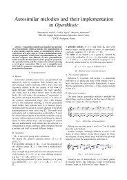
Le concept même de mélodie autosimi<strong>la</strong>ire est dû à Tom Johnson, compositeur amé-<br />
ricain vivant à Paris. L' acception mathématique du terme « autosimi<strong>la</strong>ire » est plus restrictive<br />
que celle utilisée par T. Johnson : <strong>pour</strong> rester conforme à <strong>la</strong> notion d'autosimi<strong>la</strong>rité des obj<strong>et</strong>s<br />
fractals, on dira qu'une mélodie est autosimi<strong>la</strong>ire de rapport k si, en prenant seulement une<br />
note tous les k temps, on entend <strong>la</strong> mélodie initiale (jouée k fois plus lentement). Enfin l' étude<br />
de ces mélodies particulières est aussi bien abstraite (arithmétique, algèbre commutative) que<br />
pratique (énumération exhaustive de catalogues de solutions, dénombrements, module dans<br />
15 C<strong>et</strong>te idée a été exposée <strong>pour</strong> <strong>la</strong> première fois dans Agon, C., <strong>Amiot</strong>, E., Andreatta, M., Noll, T., « Oracles for<br />
Computer-Aided. Improvisation », ICMC, New Orleans (2006). Une implémentation convaincante de ce concept de<br />
«Fourier DJ» a été présentée par Thomas Noll au dernier colloque de <strong>la</strong> SMCM en juin 2009.<br />
16 Je n'ai trouvé sur ce suj<strong>et</strong> qu'une page de David Feldman, dans sa recension de SelfSimi<strong>la</strong>r Melodies de Tom Johnson.<br />
Il y réfute bril<strong>la</strong>ment une conjecture de ce dernier concernant <strong>la</strong> conjonction de symétries par rétrogradation<br />
<strong>et</strong> inversion des mélodies autosimi<strong>la</strong>ires.<br />
p. 12
OpenMusic perm<strong>et</strong>tant, entre autres choses, <strong>la</strong> construction de mélodies autosimi<strong>la</strong>ires ayant un<br />
groupe de symétries affines données), <strong>et</strong> même philosophique (car ce sont des «obj<strong>et</strong>s univer-<br />
sels», i.e. des attracteurs limites d’itérations affines).<br />
Une mélodie autosimi<strong>la</strong>ire familière<br />
Il s'avère que c<strong>et</strong>te notion fort peu connue est <strong>pour</strong>tant profondément ancrée dans<br />
<strong>la</strong> culture musicale, fût-ce inconsciemment : on trouve des mélodies autosimi<strong>la</strong>ires aussi bien<br />
chez D. Scar<strong>la</strong>tti, Mozart, dans <strong>la</strong> cinquième symphonie de Be<strong>et</strong>hoven, que dans In the Mood de<br />
Glen Miller par exemple. Or mes calculs, en établissant qu'une mélodie donnée possède une<br />
probabilité infinitésimale d'être autosimi<strong>la</strong>ire, montrent que l'existence de mélodies autosimi-<br />
<strong>la</strong>ires, même rares, dans l'œuvre d'un compositeur, ne peut être interprétée comme le fait du<br />
hasard.<br />
Ces trois domaines de recherche sont présentés plus en détail dans le développe-<br />
ment qui suit, à travers cinq articles, choisis comme représentatifs de mon travail. On r<strong>et</strong>rou-<br />
vera, dans leur apparente diversité, <strong>la</strong> profonde unité des concepts qui les sous-tendent.<br />
p. 13
Produits de mes recherches<br />
Dans les pages qui suivent, je me propose de présenter <strong>et</strong> de détailler le contenu des<br />
cinq articles figurant dans le dossier de mes travaux, tout en les rep<strong>la</strong>çant dans le double con-<br />
texte de mes recherches personnelles <strong>et</strong> du champ de <strong>la</strong> recherche en général. En eff<strong>et</strong> mes tra-<br />
vaux individuels sont souvent liés à des réalisations collectives. En témoignent les divers arti-<br />
cles co-écrits avec d'autres chercheurs (cf. <strong>la</strong> bibliographie). Les cinq articles r<strong>et</strong>enus comme<br />
représentatifs de ma production sont:<br />
✦ « À propos des canons rythmiques », Gaz<strong>et</strong>te des Mathématiciens, 106 (2005).<br />
✦ « David Lewin and Maximally Even S<strong>et</strong>s », Journal of Mathematics and Music (2007)<br />
vol. 3.<br />
✦ « Autosimi<strong>la</strong>r Melodies », JMM (2008) vol. 3.<br />
✦ « Discr<strong>et</strong>e Fourier Transform and Bach’s Good Temperament »,<br />
Music Theory Online (2009) 15, 2.<br />
✦« New Perspectives on rhythmic canons and the Spectral Conjecture<br />
», JMM (2009).<br />
Ils touchent aux trois domaines d'étude définis dans l' Introduction: canons ryth-<br />
miques, gammes musicales, <strong>et</strong> mélodies autosimi<strong>la</strong>ires.<br />
Canons rythmiques<br />
Parmi les nombreux articles que j'ai consacrés aux canons rythmiques, le dossier<br />
joint proose les deux études suivantes:<br />
1. « À propos des canons rythmiques », Gaz<strong>et</strong>te des Mathématiciens, 106 (2005)<br />
2. « New Perspectives on rhythmic canons and the Spectral Conjecture », JMM (2009).<br />
Dans <strong>la</strong> suite du texte, ces articles seront référencés par [GdM] <strong>et</strong> [<strong>Amiot</strong>JMM].<br />
p. 14
Le premier article offre une synthèse de mes premières années de recherche sur les<br />
canons ; il présente, notamment, le résultat séminal qui perm<strong>et</strong> de limiter l'étude des conjectu-<br />
res sur les pavages de <strong>la</strong> ligne aux canons de Vuza.<br />
La formalisation musicale d'un canon rythmique (mosaïque), c'est à dire d'un pa-<br />
vage parfait périodique par un unique motif A, répété à différents intervalles de temps, se ra-<br />
mène à l'équation suivante:<br />
équation<br />
A ⊕ B = Z/nZ.<br />
(A est le motif, B représente les différents départs de ce motif) qui équivaut à l'<br />
A(X) × B(X) = 1 + X + X 2+ … X n-1 modulo X n -1 (1)<br />
où A(X), polynôme caractéristique de <strong>la</strong> partie A, est <strong>la</strong> somme des X k quand k<br />
décrit l'ensemble A. Le problème de <strong>la</strong> recherche de tous les canons rythmiques de période n<br />
donnée, se traduit donc par une question de factorisation 17 du polynôme 1 + X + X 2+ … X n-1 ,<br />
étant entendu qu'on cherche deux facteurs dont les coefficients soient exclusivement des 0 ou<br />
des 1 (appelés polynômes 0-1 dans [GdM]), <strong>et</strong> dont le produit est calculé modulo X n -1, ce qui<br />
signifie que tout monôme X k où k>n est remp<strong>la</strong>cé (itérativement) par X k-n, ce que j'ai implé-<br />
menté naturellement par pattern-matching. Je mentionne ce détail apparemment secondaire,<br />
parce qu'il est significatif de <strong>la</strong> prégnance des idées musicales à tous les stades de ces recher-<br />
ches. En eff<strong>et</strong>, c<strong>et</strong>te règle de programmation présente une signification perceptive forte, à<br />
savoir que le k ème temps du canon sera occupé par une note, qui peut fort bien appartenir à une<br />
copie du motif ayant commencé plus de n notes avant 18.<br />
17 La difficulté vient, bien évidemment, de ce que l'anneau quotient Z[X]/(X n-1) n'est pas factoriel: les factorisations<br />
n'y sont pas uniques, <strong>et</strong> en particulier il y en a d'autres que celles que l'on trouve dans les polynômes habituels.<br />
J'ai exploré une autre piste (cf. [GdM]), cherchant des factorisations modulo p premier de l'équation (1). À<br />
ma grande surprise, il se trouve que tout motif pave (<strong>pour</strong> un période suffisamment grande), au sens où tout polynôme<br />
0-1 A(x) dans Fp[X] adm<strong>et</strong> un complément B(x), lui aussi 0-1, tel que (1) soit vérifiée — modulo X p - 1.<br />
18 L' auditeur perçoit des pavages de <strong>la</strong> ligne temporelle <strong>et</strong> non pas du cercle, structure quotient. Mais mathématiquement<br />
les deux notions sont identiques, tout pavage de <strong>la</strong> ligne par trans<strong>la</strong>tions d'un motif étant périodique.<br />
p. 15
Nous rencontrerons d'autres exemples de c<strong>et</strong>te utilité d'une culture musicale à pro-<br />
pos de questions qui sembleraient relever des mathématiques les plus abstraites.<br />
pavage de Z <strong>et</strong> de Z/12Z par le motif {0,1,5}<br />
Les facteurs irréductibles dans Z[X] du polynôme 1 + X + X 2+ … X n-1 sont bien connus, ce sont<br />
les polynômes cyclotomiques Φd où d divise n. Certains de ces polynômes sont 0-1; c'est le cas,<br />
par exemple, quand d est premier <strong>et</strong> Φd = 1 + X +… X d-1. D'autres ne le sont pas, comme Φ12 = 1-<br />
X 2+X 4. C<strong>et</strong>te remarque, qui date de <strong>la</strong> préhistoire de l'étude des pavages, a permis d'implémen-<br />
ter dans OpenMusic un "patch" de production de canons rythmiques, dits « canons cyclotomi-<br />
ques 19 » : <strong>pour</strong> obtenir des canons de période n, il suffit de sélectionner parmi les parties de<br />
l'ensemble des diviseurs d1 … dk de n celles qui fournissent un polynôme 0-1 par le produit des<br />
facteurs cyclotomiques Φd i correspondants, ce qui créera ipso facto un canon rythmique 20, à con-<br />
dition que ce polynôme A(X) adm<strong>et</strong>te un complément B(X) — un polynôme 0-1 lui aussi, <strong>et</strong> qui vérifie<br />
l'équation (1). Ainsi <strong>pour</strong> n=12<br />
A(X) = Φ2 Φ4 Φ12 = (1 + X)(1 + X 2)(1 - X 2 + X 4) = 1 + X + X 6 + X 7<br />
est un polynôme 0-1, correspondant à <strong>la</strong> partie A = {0,1,6,7} qui "pave" (i.e. constitue<br />
un canon rythmique) avec par exemple B = {0, 2, 4} i.e. B(X) = 1 + X 2 + X 4.<br />
Le problème posé par c<strong>et</strong>te démarche tient à ce que fabriquer un polynôme 0-1<br />
A(X), fût-il produit de polynômes cyclotomiques, ne garantit pas l'existence d'un complément<br />
B(X). Ainsi <strong>pour</strong> :<br />
19 Agon, C., <strong>Amiot</strong>, E., Andreatta, M., « Tiling the (musical) line with polynomials : Some theor<strong>et</strong>ical and implementa-<br />
tional aspects », Acts of ICMC 2005, Barcelona (2005).<br />
20 Mais ce canon n'est jamais un canon de Vuza: l'algorithme utilisé, qui est emprunté à Coven <strong>et</strong> Meyerowitz,<br />
donne toujours un complément B périodique.<br />
p. 16
A = {0,1,2,4,5,6}, i.e. A(X) = (1 + X 4)(1 + X + X 2) = Φ8 Φ3<br />
il n'existe pas de pavage de Z/12Z — ni d'ailleurs d'aucun Z/nZ — dont le motif<br />
soit A. Ce fait résulte des conditions qui se trouvent exposées dans l'article séminal [CM], <strong>et</strong><br />
qui sont les premières conditions générales que l'on ait publiées <strong>pour</strong> que l'équation (1) soit vé-<br />
rifiée. Ces conditions, (T1) <strong>et</strong> (T2), portent précisément sur les indices des facteurs cyclotomi-<br />
ques du polynôme caractéristique A(X) d'une partie A de Z: si on note RA l'ensemble des indi-<br />
ces d des Φd qui divisent A(X), <strong>et</strong> SA le sous-ensemble des éléments de RA qui sont des puissan-<br />
ces de nombres premiers, alors ces conditions s'énoncent ainsi :<br />
✦ (T1) : <strong>la</strong> valeur A(1) est le produit des Φpk(1) <strong>pour</strong> chaque p k dans SA.<br />
✦ (T2) : <strong>pour</strong> chaque p k , q l … dans SA, on a p k × q l ×…. qui appartient à RA.<br />
En 1998, Coven <strong>et</strong> Meyerowitz ont prouvé 21 que<br />
vérifiée.<br />
✦ Si A pave, alors (T1) est vérifiée.<br />
✦ Si (T1) <strong>et</strong> (T2) sont vérifiées, alors A pave.<br />
✦ Si A pave Z/n Z où n a au plus deux facteurs premiers, alors (T2) aussi est<br />
On ignore encore si c<strong>et</strong>te dernière propriété est vraie <strong>pour</strong> tout n. J'ai prouvé dans<br />
[<strong>Amiot</strong>JMM] que tous les canons de Vuza de période 120 vérifient (T2), ce qui implique que<br />
c<strong>et</strong>te propriété est vraie <strong>pour</strong> une infinité d'autres canons. En eff<strong>et</strong>, ainsi que je l'avais démon-<br />
tré précédemment 22,<br />
Tout canon rythmique peut se décomposer récursivement en canons plus courts, jusqu'à ce que<br />
l'on arrive à un canon de Vuza;<br />
Et, en conséquence 23, <strong>la</strong> condition (T2) étant conservée durant ces tribu<strong>la</strong>tions,<br />
La conjecture « pave ⇒ (T2) » est vraie <strong>pour</strong> tout canon si, <strong>et</strong> seulement si, e(e est vraie<br />
<strong>pour</strong> tous les canons de Vuza.<br />
21 Leur article sera dorénavant cité comme [CM].<br />
22 « Rhythmic canons and Galois Theory », actes du Colloquium on Mathematical Music Theory, H. Fripertinger<br />
& L. Reich Eds, Grazer Math. Bericht Nr 347 (2005). Cité comme [<strong>Amiot</strong>05].<br />
23 Les calculs polynomiaux sont un peu longs, mais restent élémentaires, cf. ibid.<br />
p. 17
Edouard Gilbert [Gil] a parachevé <strong>la</strong> démonstration de ce théorème, que j'avais<br />
énoncé sans prendre <strong>la</strong> peine d'en donner <strong>la</strong> preuve dans [GdM]. Il est notable que<br />
<strong>et</strong> Meyerowitz.<br />
(T1) + (T2) ⇒ spectral,<br />
ce qui a été démontré par Izabel<strong>la</strong> Łaba 26, peu après qu'elle ait lu l'article de Coven<br />
Les canons de Vuza, obj<strong>et</strong>s musicaux par excellence, sont ainsi devenus incontour-<br />
nables <strong>pour</strong> <strong>la</strong> résolution de conjectures fondamentales de mathématiques pures. Le second<br />
article présenté en annexe répond à une question pointue <strong>et</strong> ésotérique: il s'agit de déterminer<br />
tous les canons de Vuza de période n=120, complétant ainsi <strong>la</strong> recherche présentée par Ko-<br />
lountzakis <strong>et</strong> Matolcsi 27 dans le même numéro du Journal for Mathematics and Music par <strong>la</strong> c<strong>la</strong>s-<br />
sification exhaustive de ces canons <strong>pour</strong> les périodes inférieures à 168, <strong>et</strong> ce <strong>pour</strong> mieux étudier<br />
certaines des conjectures évoquées ci-dessus. Ce numéro spécial du Journal for Mathematics and<br />
Music de 2009 consacré aux canons rythmiques fait <strong>la</strong> part belle à <strong>la</strong> conjecture de Fuglede:<br />
c'est le suj<strong>et</strong> du troisième article (de Franck Jedrzejewski), elle est citée dans [KM], <strong>et</strong> démon-<br />
trée au passage <strong>pour</strong> n=120 par [<strong>Amiot</strong>JMM] 28. Notons que ce<strong>la</strong> prouve aussi <strong>la</strong> conjecture de<br />
Fuglede 29 <strong>pour</strong> tout canon de période 240 (par exemple) qui n'est pas un canon de Vuza: en<br />
eff<strong>et</strong>, il se décompose alors en canons plus p<strong>et</strong>its 30, qui vérifient donc nécessairement <strong>la</strong> conjec-<br />
ture spectrale puisqu'elle est vraie <strong>pour</strong> n≤120.<br />
La démarche, commune à ces deux derniers articles (avec n=144 dans [KM]) a été<br />
proposée par Maté Matolcsi. Elle consiste à c<strong>la</strong>ssifier les canons de Vuza par leurs ensembles<br />
SA, en utilisant l'algorithme suivant:<br />
✦ Choisir un SA qui perm<strong>et</strong>te d'espérer un canon de Vuza (des conditions sur RA<br />
perm<strong>et</strong>tent de repèrer <strong>la</strong> périodicité de A, voire celle de son complément éventuel B, cf. [KM]).<br />
26 Laba, I., « The spectral s<strong>et</strong> conjecture and multiplicative properties of roots of polynomials », J. London<br />
Math. Soc. 65, pp. 661–671 (2002).<br />
27 Dorénavant citée comme [KM].<br />
28 Les résultats de Coven-Meyerowitz <strong>et</strong> Laba suffisaient à établir <strong>pour</strong> n=144 que « pave ⇒ spectral ».<br />
29 Au moins dans le sens « pave ⇒ spectral ».<br />
30 Des canons dont <strong>la</strong> période divise strictement 240, donc est au plus égale à 120.<br />
p. 19
✦ Fabriquer par l'algorithme de Coven <strong>et</strong> Meyerowitz un B qui complète tous les<br />
A possibles ayant c<strong>et</strong> ensemble SA.<br />
que (1) soit vérifiée.<br />
✦ Rechercher tous les compléments de ce complément, i.e. tous les motifs A tels<br />
✦ Trier par les valeurs de l'ensemble RA — incidemment, ceci perm<strong>et</strong> de nouveau<br />
d'éliminer des canons non Vuza.<br />
✦ Sélectionner les solutions non périodiques, s'il y en a.<br />
C<strong>et</strong> algorithme nous a permis (avec quelques ruses de programmation <strong>pour</strong> les cas<br />
les plus coriaces) de produire <strong>la</strong> c<strong>la</strong>ssification suivante des canons de Vuza de période 72, 108,<br />
120 ou 144, les deux premières périodes ayant déjà été exhaustivement détaillées par Harald<br />
Fripertinger [Frip]:<br />
n RA RB nombre de ≠A nombre de ≠B<br />
72 {2, 8, 9, 18, 72} {3, 4, 6, 12, 24, 36} 6 3<br />
108 {3, 4, 12, 27, 108} {2, 6, 9, 18, 36, 54} 252 3<br />
120 {2, 3, 6, 8, 15, 24, 30, 120} {4, 5, 10, 12, 20, 40, 60} 20 16<br />
120 {2, 5, 8, 10, 15, 30, 40, 120 {3, 4, 6, 12, 20, 24, 60} 18 8<br />
144<br />
144<br />
144<br />
144<br />
{2,8,9,16,18,24,72,144}<br />
or {2,8,9,16,18,72,144}<br />
{2, 4, 9, 16, 18, 36, 144} or<br />
{2, 4, 6,9, 16, 18, 36, 144} or<br />
{2, 4, 9, 12, 16, 18, 36, 144}<br />
{3, 4, 6, 8, 12, 24, 48, 72} or<br />
{3, 4, 6, 8, 12, 24, 36, 48, 72}<br />
{2, 3, 6, 8, 12, 24, 48, 72} or<br />
{2, 3, 6, 8, 12, 18, 24, 48, 72}<br />
{3,4,6,12,24,36,48} 36 6<br />
{3,6,8,12,24,36,72} 8640 3<br />
{2,9,16,18,144} or<br />
{2,9,16,18,36,144}<br />
156<br />
+6<br />
48<br />
+12<br />
{4, 9, 16, 18, 36, 144} 324 6<br />
p. 20<br />
Il n'y avait pas là de canons inédits <strong>pour</strong> n=120 (ceux qui ne provenaient pas de l'al-<br />
gorithme de Vuza avaient été façonnés empiriquement à partir de canons de période 72), mais<br />
l'algorithme utilisé a permis de l'établir avec certitude; en revanche de nouveaux canons ont été<br />
trouvés <strong>pour</strong> n=144, montrant au passage (dans l'avant-dernier cas) qu'on pouvait avoir plu
sieurs ensembles RA en face de plusieurs ensembles RB distincts (même si SA <strong>et</strong> SB ne peuvent<br />
changer, d'après [CM]).<br />
Par ailleurs, j'ai utilisé depuis <strong>et</strong> utilise encore une version rapide de ce "ping-pong"<br />
entre voix de canons <strong>pour</strong> tester des canons de plus grande taille <strong>et</strong> voir s'ils vérifiaient <strong>la</strong> con-<br />
dition (T2), en utilisant <strong>la</strong> programmation linéaire <strong>pour</strong> chercher un complément de B (renon-<br />
çant à les chercher tous, ce qui est trop coûteux en temps de calcul). L' idée m'en est venue en<br />
travail<strong>la</strong>nt sur des problèmes de décomposition linéaires de gammes, exactes ou approchées,<br />
avec Bill S<strong>et</strong>hares [AS]. Le problème n'avait rien à voir a priori avec les pavages, mais <strong>la</strong> pro-<br />
grammation linéaire fournissait une méthode rapide (<strong>et</strong> quasi infaillible) <strong>pour</strong> obtenir un com-<br />
plément B d'un motif A qui pave 31. En itérant l'algorithme, on trouve un complément A' de B,<br />
puis un complément B' de A', <strong>et</strong>c… jusqu'à r<strong>et</strong>omber sur un motif (ou complément) déjà expri-<br />
mé. Les ensembles SA <strong>et</strong> SB restent invariants tout au long de <strong>la</strong> procédure. C<strong>et</strong>te exploration<br />
avait <strong>pour</strong> but de trouver des canons de Vuza qui ne vérifiraient pas <strong>la</strong> condition (T2), ni peut-<br />
pas <strong>la</strong> condition spectrale; mais elle a failli à fournir un tel contre-exemple <strong>pour</strong> toutes les pé-<br />
riodes al<strong>la</strong>nt jusqu'à n=1200 32.<br />
En eff<strong>et</strong>, <strong>la</strong> procédure décrite dans le numéro spécial de JMM présente deux points<br />
faibles: le calcul de tous les compléments prend du temps, même après les diverses optimisa-<br />
tions apportées par Matolcsi, lesquelles sont <strong>pour</strong>tant particulièrement pertinentes <strong>pour</strong> des<br />
canons "irréguliers" comme ceux de Vuza; le calcul de l'ensemble RA est long lui aussi.<br />
Pour réduire le temps de calcul de c<strong>et</strong>te dernière tâche, j'ai suivi une suggestion de<br />
Matolcsi <strong>et</strong> calculé certaines valeurs particulières du polynôme A(X) aux points X = e 2 i k π/n. En<br />
eff<strong>et</strong>, ces valeurs ne sont autres que <strong>la</strong> transformée de Fourier (discrète) de l'ensemble A, qui<br />
perm<strong>et</strong> de déceler en particulier ses périodicités internes. On obtient notamment<br />
31 Qui plus est, l'algorithme du simplexe étant fortement asymétrique, il tend à donner des solutions non périodiques,<br />
c'est à dire qu'on trouve des canons de Vuza quand il y en a <strong>pour</strong> les couples SA <strong>et</strong> SB considérés.<br />
32 Ceci ne constitue pas une preuve de ce qu'il n'y ait pas de tels contre-exemples avec de "p<strong>et</strong>ites" périodes, mais<br />
le <strong>la</strong>isse conjecturer, dans <strong>la</strong> mesure où les listes de canons de Vuza ainsi formées ont des cardinaux simi<strong>la</strong>ires à ce<br />
que l'on trouve dans les cas où le catalogue exhaustif est connu. Il est probable que de tels contre-exemples n'existent<br />
que <strong>pour</strong> d'assez grandes périodes, mais il serait dommage de se priver d'explorer les périodes qui nous sont<br />
d'ores <strong>et</strong> déjà accessibles.<br />
p. 21
(ou une gamme) remonte à David Lewin en 1959. <strong>et</strong> est à l’origine de nombreux concepts qui ont marqué <strong>la</strong><br />
recherche américaine depuis 1959. Nous choisissons <strong>la</strong> même définition que lui parmi les diverses définition<br />
possibles équivalentes :<br />
Définition 1. La transformée de Fourier de f : Zc → C est<br />
F(f) :t ↦→<br />
Z/cZ qui modélise <strong>la</strong> gamme chromatique, il s'agit d'une transformée de Fourier discrète, ou<br />
<br />
f(k)e −2ikπt/c<br />
p. 23<br />
k∈Zc<br />
Plus<br />
DFT:<br />
particulièrement, <strong>la</strong> transformée de Fourier de A ⊂ Zc sera <strong>la</strong> transformée de Fourier de <strong>la</strong> fonction<br />
caractéristique 1A du sous-ensemble A5 :<br />
FA : t ↦→ <br />
e −2iπkt/c<br />
k∈A<br />
Quelques exemples :<br />
(1) FZc, <strong>la</strong> transformée de Fourier de toute <strong>la</strong> gamme chromatique, est d−1 <br />
e<br />
k=0<br />
−2iπkt/c Le premier qui ait utilisé c<strong>et</strong>te DFT à des fins d'étude structurelle en théorie de <strong>la</strong><br />
1 − e−2iπt<br />
musique est sans nul doute David Lewin, dans son tout premier = . C<strong>et</strong>te<br />
1 − e−2iπt/c fonction est nulle sur Zc sauf quand t = 0. On voit bien sur ce calcul que seule compte <strong>la</strong> c<strong>la</strong>sse de<br />
l’indice k modulo d, ce qui est adéquat.<br />
33 ainsi que dans son dernier<br />
article34. Dans le premier cas, il n'y fait qu'une allusion in fine, s'excusant de <strong>la</strong> difficulté de no-<br />
tions comme l'algèbre des caractères <strong>pour</strong> les lecteurs du Journal of Music Theory. Néanmoins,<br />
4On prend le double du sinus de l’intervalle, avec un facteur d’échelle. . .<br />
5 1 Si l’on s’intéresse aux fonctions du cercle S à valeurs dans C, on peut voir ce<strong>la</strong> comme <strong>la</strong> transformée de Fourier d’une<br />
distribution, à savoir un peigne de Dirac <br />
k∈A δk.<br />
toute son analyse des rapports intervalliques entre deux parties de Z/nZ (qu'on n'appe<strong>la</strong>it pas<br />
2 title on some pages<br />
encore des pitch-c<strong>la</strong>ss s<strong>et</strong>s ou pc-s<strong>et</strong>s) repose sur les re<strong>la</strong>tions entre leurs transformées de Fourier.<br />
This shows that (when the Fourier transform of the characteristic function of A is non vanishing) knowledge<br />
of A andEn ofeff<strong>et</strong>, the interval si <strong>pour</strong> function deux parties yieldsA, compl<strong>et</strong>e B de Z/nZ knowledge on définit of the<strong>la</strong> characteristic fonction d'intervalles function ofpar B.<br />
Defining the interval function b<strong>et</strong>ween A, B ⊂ Zc as<br />
IFUNC(A, B)(t) = nombre d'intervalles de taille t entre une note de A <strong>et</strong> une note de<br />
IF unc(A, B)(t) = Card{(a, b) ∈ A × B, b − a = t},<br />
B,<br />
<br />
il s'avère que c<strong>et</strong>te fonction est le produit 1 if t ∈de X<br />
the characteristic fuction of X as 1X(t) =<br />
convolution , IF unc appears des fonctions immediately caractéristi- as the convolution<br />
0 if t/∈ X<br />
ques product de -A <strong>et</strong> ofde theB: characteristic functions of −A and B:<br />
1−A ⋆ 1B : t ↦→ <br />
1−A(k)1B(t − k) = <br />
2 title on some pages<br />
This shows that (when the Fourier transform of the characteristic function of A is non vanishing) knowledge<br />
of A and of the interval function yields compl<strong>et</strong>e knowledge of the characteristic function of B.<br />
Defining the interval function b<strong>et</strong>ween A, B ⊂ Zc as<br />
IF unc(A, B)(t) = Card{(a, b) ∈ A × B, b − a = t},<br />
<br />
1 if t ∈ X<br />
the characteristic fuction of X as 1X(t) =<br />
, IF unc appears immediately as the convolution<br />
0 if t/∈ X<br />
product of the characteristic functions of −A and B:<br />
1−A ⋆ 1B : t ↦→<br />
1A(k)1B(t + k) =IF unc(A, B)(t)<br />
<br />
1−A(k)1B(t − k) =<br />
k∈Zc<br />
<br />
1A(k)1B(t + k) =IF unc(A, B)(t)<br />
k∈Zc<br />
k∈Zc<br />
as 1A(k)1B(t + k) is nil except when k ∈ A and t + k ∈ B. Hence from the general formu<strong>la</strong> for the Fourier<br />
as transform 1A(k)1B(t Or of <strong>la</strong> + aDFT convolution k) isdu nilproduit except product, when de convolution k ∈ A and t est + kle ∈produit B. Hence ordinaire from thedes general DFT: formu<strong>la</strong> for the Fourier<br />
transform of a convolution product,<br />
F(IF unc(A, B)) = F(1−A) × F(1B)<br />
F(IF unc(A, B)) = F(1−A) × F(1B)<br />
where F(f) stands for the discr<strong>et</strong>e Fourier transform of a map f.<br />
Ce<strong>la</strong> signifie qu'il est possible de récupérer B, connaissant A <strong>et</strong> IFUNC(A, B) —<br />
where We will F(f) not stands quotefor the the formu<strong>la</strong> discr<strong>et</strong>e given Fourier by Lewin transform himself, of aas map it isf. hardly understandable: his notations are<br />
sauf<br />
undefined<br />
quand We will <strong>la</strong> not and<br />
DFT quote the<br />
de<br />
computations<br />
A the a formu<strong>la</strong> <strong>la</strong> mauvaise given extremely<br />
grâce by Lewin cursory.<br />
de s'annuler, himself, Of course as ce itqui this is hardly arrive<br />
is notunderstandable: dans<br />
for <strong>la</strong>ck<br />
le cas<br />
of rigor:<br />
des his «special<br />
as notations the following are<br />
undefined quotation and suggests, the computations Lewin did not extremely really hope cursory. to beOf understood course this when is not making for <strong>la</strong>ck useofofrigor: mathematics. as the following<br />
cases» quotation The énumérés mathematical suggests, par Lewin reasoning (telles didby not which <strong>la</strong> really gamme I arrived hope par to at tons, be this understood result ou <strong>la</strong> is gamme notwhen communicable mélodique making use tomineure aofreader mathematics. ascen- who does not<br />
The havemathematical considerable mathematical reasoning by training. which I arrived For those at this who result have such is not a training, communicable I append to a areader sk<strong>et</strong>ch who of the does proof not:<br />
dante have (0 consider 2 3 considerable 5 7 the 9 11)). groupmathematical algebra [. . . ] [13] training. For those who have such a training, I append a sk<strong>et</strong>ch of the proof :<br />
Reading consider the Lewin’s grouppaper algebra gives [. . . ] one [13] a strong feeling that he wrote as little as possible on the mathematical<br />
tools Reading that under<strong>la</strong>y Lewin’s paper his results. gives one Indeed, a strong whatfeeling little he that mentioned he wrotedid as little rouseas some possible readers on to therighteous mathematical ire in<br />
tools the DFT next that <strong>et</strong> issue "Maximally under<strong>la</strong>y of JMT. his results. Even Indeed, S<strong>et</strong>s" what little he mentioned did rouse some readers to righteous ire in<br />
theNowadays next issuesuch of JMT. a ‘considerable mathematical training’ will be considered basic by many readers of this<br />
journal; Nowadays for instance such a ‘considerable D.T. Vuza made mathematical an essential training’ use ofwill the be equation considered above basic in the by many 80’s inreaders the course of this of<br />
journal; his seminal for work instance about D.T. rhythmic Vuza made canons an(see essential [21], lemma use of the 1.9 sqq), equation wherein above heinstressed the 80’s the inimportance the course of<br />
his Lewin’s seminal usework of DFT about of characteristic rhythmic canons functions. (see [21], lemma 1.9 sqq), wherein he stressed the importance of<br />
33 Lewin, Lewin’s And D., as Re: use we Intervallic ofwill DFT endeavour Re<strong>la</strong>tions of characteristic to b<strong>et</strong>ween prove, functions. two thiscollections approachof enables notes, Journal to define of Music ME Theory, s<strong>et</strong>s (in3:298-301 equal temperament) (1959). in<br />
a way And perhaps as we will more endeavour suggestive to prove, and even thisintuitive, approachthan enables historical/usual to define MEdefinitions. s<strong>et</strong>s (in equal temperament) in<br />
34 Lewin, D., Special Cases of the Interval Function b<strong>et</strong>ween Pitch-C<strong>la</strong>ss S<strong>et</strong>s X and Y, Journal of Music Theory,<br />
45-129<br />
a way<br />
(2001).<br />
perhaps more suggestive and even intuitive, than historical/usual definitions.<br />
k∈Zc<br />
1.2 A quick summary of Fourier transforms of subs<strong>et</strong>s of Zc<br />
1.2 A quick summary of Fourier transforms of subs<strong>et</strong>s of Zc<br />
1.2.1 First moves.<br />
1.2.1 Definition First1.1 moves. Following Lewin, we will define the Fourier transform of a pc-s<strong>et</strong> A ∈ Zc as the Fourier<br />
transform of its characteristic function 1A:
Le cas particulier B=A a été réexaminé de manière magistrale dans sa thèse 35 par Ian<br />
Quinn , qui voulut reconnaître, par les propriétés de leurs coefficients de Fourier, les parties les<br />
plus «prototypales» , i.e. celles qui jouent le rôle de phares dans le paysage des accords. La dé-<br />
couverte <strong>la</strong> plus remarquable de Quinn est que ces «phares» ou prototypes, consacrés par <strong>la</strong> cri-<br />
tique traditionnelle, sont caractérisés par <strong>la</strong> valeur maximale de l'un de leurs coefficients de<br />
Fourier. Or les prototypes en question ne sont autres que les Maximally Even S<strong>et</strong>s ou ME S<strong>et</strong>s,<br />
que je traduis par «gammes bien réparties» dans mon article <strong>pour</strong> <strong>la</strong> Revue de mathématiques <strong>et</strong><br />
sciences humaines 36; ce sont les répartitions de notes les plus proches d'un polygone régulier: ainsi<br />
A<br />
A<br />
G<br />
<strong>la</strong> collection diatonique est, parmi les parties à sept notes de <strong>la</strong><br />
gamme chromatique, celle qui se rapproche le mieux<br />
d'un heptagone régulier (cf. <strong>la</strong> figure ci-jointe).<br />
Évidemment, il convient de préciser ce qu'on<br />
entend précisément par «se rapprocher<br />
d'un polygone régulier». Douth<strong>et</strong>t <strong>et</strong> Kranz<br />
ont prouvé qu'en termes de potentiels sur un<br />
cercle discr<strong>et</strong>, toutes les fonctions potentiel<br />
strictement convexes (comme les potentiels coulom-<br />
biens en physique) donnaient les mêmes ME S<strong>et</strong>s 37. Or<br />
Quinn a mis en évidence, dans sa thèse, une autre manière d'apprécier <strong>la</strong> «bonne répartition»:<br />
Le pc-s<strong>et</strong> A à d éléments est « bien réparti » si, <strong>et</strong> seulement si, <strong>la</strong> valeur |FA(d)| (ampli-<br />
tude du d ème coefficient de Fourier) est maximale par rapport à tous les autres pc-s<strong>et</strong>s à d élé-<br />
ments.<br />
B<br />
G<br />
C<br />
C major<br />
F<br />
C<br />
F<br />
D<br />
E<br />
D<br />
p. 24<br />
35 Quinn, I., « A unified theory of chord quality in equal temperaments », PhD dissertation, Univ. of Rochester<br />
(2005).<br />
36 <strong>Amiot</strong>, E., « Gammes Bien Réparties », Revue de Mathématiques <strong>et</strong> Sciences Humaines, 178 (juill<strong>et</strong> 2007).<br />
37 Douth<strong>et</strong>t, J. <strong>et</strong> Krantz, R. « Energy extremes and spin configurations for the one-dimensional antiferromagn<strong>et</strong>ic<br />
Ising model with arbitrary-range interaction », Journal of Mathematical Physics 37 (1996).
Mon article du Journal of Mathematics and Music, joint dans le dossier annexe 38, dé-<br />
montre rigoureusement tout en <strong>la</strong> généralisant, c<strong>et</strong>te découverte de Quinn. En eff<strong>et</strong>, il m'a paru<br />
nécessaire de prouver précisément 39 le fondement géométrique de c<strong>et</strong>te propriété, qui est un<br />
lemme trigonométrique (appelé « Huddling Lemma » dans [MES<strong>et</strong>s]), notamment <strong>pour</strong> c<strong>la</strong>-<br />
rifier le cas plus délicat des multi-ensembles qui apparaissent dans le cas des ME S<strong>et</strong>s dégéné-<br />
rés — comme <strong>la</strong> gamme octatonique par exemple.<br />
Au passage, j'ai démontré une conjecture de Quinn concernant certains ME s<strong>et</strong>s<br />
particuliers (ceux de type III dans sa nomenc<strong>la</strong>ture — c<strong>et</strong>te propriété ne figure pas dans l'arti-<br />
cle du JMM, mais on peut <strong>la</strong> trouver dans celui de <strong>la</strong> Revue de Mathématiques <strong>et</strong> Sciences Humai-<br />
nes); j'ai également complètement décrit tous les cas de maximalité de tous les coefficients de<br />
Fourier des pc-s<strong>et</strong>s, <strong>et</strong> r<strong>et</strong>rouvé alors de manière élégante le théorème de l'hexacorde de Babbit<br />
(avec diverses généralisations, en particulier à tout groupe abélien compact) 40. Ce dernier<br />
point, vu l'argument utilisé, mérite d'être approfondi ici : quand on prend B=A dans les équa-<br />
tions ci-dessus, on obtient le contenu intervallique de A, IC(A) en lieu <strong>et</strong> p<strong>la</strong>ce de IFUNC(A,<br />
B) (c'est l'histogramme des intervalles présents entre les notes de A, ou, comme l'exprimait jo-<br />
liment Lewin dans un de ses derniers articles, <strong>la</strong> probabilité que tel intervalle soit ouï si l'on<br />
joue des notes de A au hasard). De plus, <strong>la</strong> DFT de c<strong>et</strong> histogramme donne le module alternative au title carré<br />
(i.e. l'amplitude) de <strong>la</strong> DFT de A:<br />
Proof If A ∈ Zc has c/2 elements, then as mentioned above, F Zc\A = −FA<br />
F(ICA) =|FA| 2 = |F Zc\A| 2 = F(IC Zc\A) Hence (by inverse D<br />
C<strong>et</strong>te formule perm<strong>et</strong> de comparer As far astrès I know, facilement this short le contenu proof was intervallique first published de A in <strong>et</strong> [1] after I men<br />
memorial days in july 2005. But considering the coincidence in time of Lew<br />
celui de son complémentaire, ce qui est with précisément Babbitt, it is l'énoncé almost certain du théorème that hede was l'hexacorde. aware of it. Plus Perhaps the har<br />
in his first paper exp<strong>la</strong>in why he did not publish it. It is left to the read<br />
exercise, to prove in the same way the Generalized Hexachord Theorem,<br />
and many others.<br />
38 « David Lewin and Maximally Even S<strong>et</strong>s », Journal of Mathematics and Music (2007) vol. 3.<br />
Ci-après cité comme [MES<strong>et</strong>s].<br />
2 Maximally Even S<strong>et</strong>s and their Fourier Transforms<br />
The attribute ‘maximally even’ applies to pitch c<strong>la</strong>ss s<strong>et</strong>s, which — in com<br />
the same cardinality — are as evenly as possible distributed within Zc. Thi<br />
regu<strong>la</strong>r s<strong>et</strong>s, which exist only for cardinalities d dividing the number c of pi<br />
case — where d and c are mutually coprime — was well studied in [8].<br />
extensive study of the general case in [7] is an explicit construction of gen<br />
formu<strong>la</strong> for this construction was <strong>la</strong>ter termed J-function. It departs from<br />
numbers 0, c<br />
c<br />
, ..., (d − 1)<br />
d d and ‘digitizes’ them within Zc in terms of the re<br />
of these ratios mod c: 0, 39 Les évidences sont bien souvent trompeuses. J'ai récemment élucidé le nombre de générateurs possibles d'une<br />
gamme monogène (comme <strong>la</strong> gamme majeure ou <strong>la</strong> gamme pentatonique, engendrées par des quintes), qui porte<br />
bien mal son nom puisque (contrairement aux parties monogènes, alias séquences arithmétiques, dans R par<br />
exemple) ce nombre peut être arbitrairement grand — mais n'est jamais égal à 14 par exemple, cf. mon article<br />
« On the number of generators of a musical scale », http://arxiv.org/abs/0909.0039.<br />
40 Ce point a été publié indépendamment dans <strong>la</strong> revue de vulgarisation mathématique Quadrature. Par ailleurs j'ai<br />
récemment étendu le théorème de l'hexacorde à des groupes compacts non nécessairement commutatifs (non publié).<br />
c c <br />
, ..., (d − 1) mod c. The J-function includ<br />
d<br />
d<br />
p. 25<br />
J α c,d : k ↦→ kc + α<br />
,k =0. . . d − 1.<br />
d
généralement, on voit sur c<strong>et</strong>te dernière formule que <strong>la</strong> connaissance de l'amplitude de <strong>la</strong><br />
DFT équivaut très exactement à <strong>la</strong> connaissance de IC(A), i.e. du contenu intervallique de<br />
A.<br />
Or l'étude des vecteurs d'intervalle, dans les années 60, a mis en lumière le fait<br />
troub<strong>la</strong>nt que certains pc-s<strong>et</strong>s ont même distribution intervallique, sans être <strong>pour</strong> autant con-<br />
gruents 41. Ces exceptions, rares, ont été baptisées « Z-re<strong>la</strong>tion » par Allen Forte. La formule<br />
secrète utilisée par Lewin rend donc compte très simplement de c<strong>et</strong>te re<strong>la</strong>tion, qui exprime<br />
l'égalité des longueurs des coefficients de Fourier.<br />
Or c'est seulement récemment que l'on s'est aperçu que c<strong>et</strong>te notion était bien<br />
connue depuis <strong>la</strong> fin des années 40 par les cristallographes, qui l'avaient nommée homométrie 42.<br />
Le problème de trouver des figures homométriques dans un groupe cyclique demeure, encore<br />
aujourd'hui, le suj<strong>et</strong> d'actives recherches, au centre desquelles je me suis subitement trouvé im-<br />
pliqué, par le biais de ces questions de ME s<strong>et</strong>s. L' une de mes dernières contributions, toute<br />
récente, est n<strong>et</strong>tement plus technique que <strong>la</strong> démonstration élégante du théorème de l'hexa-<br />
corde susmentionnée. Elle porte sur certaines unités spectrales, obj<strong>et</strong>s mystérieux qui perm<strong>et</strong>tent<br />
de générer des c<strong>la</strong>sses d'obj<strong>et</strong>s homométriques — qui, malheureusement, ne sont pas en géné-<br />
ral de vrais ensembles, mais des multi-ensembles 43. C'est en travail<strong>la</strong>nt avec Bill S<strong>et</strong>hares sur<br />
une autre présentation des re<strong>la</strong>tions entre pc-s<strong>et</strong>s 44 que j'ai trouvé un théorème pointu, qui<br />
énumère les unités spectrales rationnelles d'ordre fini. Notre proj<strong>et</strong> était de décrire des re<strong>la</strong>-<br />
tions de combinaisons linéaires entre gammes (ou accords, plus exactement). Par exemple<br />
Do mineur = Do majeur - Fa majeur + Mib majeur.<br />
p. 26<br />
Pour ce faire, nous avons introduit un formalisme matriciel, qui n'est autre qu'une<br />
représentation (au sens vulgaire comme au sens de <strong>la</strong> théorie des représentations de groupes)<br />
41 i.e. isomorphes au groupe T/I près : il est évident que transposer, ou inverser, un pc-s<strong>et</strong> A ne change pas ICA.<br />
42 En eff<strong>et</strong>, l'observation de <strong>la</strong> figure de diffraction donnée par un solide éc<strong>la</strong>iré par des rayons X est essentiellement<br />
équivalente à l'amplitude de sa transformée de Fourier. Les solides homométriques mais non congruents<br />
sont donc des obstacles à une reconnaissance taxonomique via l'observation par ces techniques.<br />
43 « On the Group of Rational Spectral Units with Finite Order », http://arxiv.org/abs/0907.0857.<br />
44 « An Algebra for periodic rhythms and scales ». À paraître chez Springer.
<strong>et</strong> de considérer les DFT des applications k→ uk définies d'un groupe cyclique Z/n<br />
Z dans le corps des nombres complexes. Une élégante propriété établie par Noll est que, dans<br />
le cas d'une telle gamme monogène, les coefficients de Fourier sont tous alignés en tant que<br />
nombres complexes dans le p<strong>la</strong>n d'Argan-Cauchy, comme on le voit sur <strong>la</strong> figure suivante 47.<br />
6<br />
1<br />
4<br />
560123<br />
3<br />
Une gamme <strong>et</strong> ses coefficients de Fourier<br />
Pour aller plus loin, j'ai plus généralement examiné une partie finie, fixée de S 1 (on<br />
peut considérer de manière typique douzes notes obtenues par itération de <strong>la</strong> quinte pythago-<br />
ricienne à partir d'une fondamentale) qu'on peut voir comme une gamme chromatique non né-<br />
cessairement tempérée, <strong>et</strong> les gammes majeures, définies c<strong>la</strong>ssiquement comme les séquences<br />
de notes indexées par (0,2,4,5,7,9,11) ou les trans<strong>la</strong>tés modulo 12 de c<strong>et</strong> ensemble d'indices, dans<br />
<strong>la</strong> gamme chromatique ambiante.<br />
Une variante du résultat de Quinn dans ce contexte é<strong>la</strong>rgi, mais de démonstration<br />
tout à fait simi<strong>la</strong>ire, donne que parmi toutes les gammes à 7 notes, ce sont les gammes majeures<br />
qui ont <strong>la</strong> plus grande valeur de leur premier coefficient de Fourier a1 — ce sont les plus pro-<br />
47 J'ai bien entendu étudié <strong>la</strong> réciproque, qui se trouve être <strong>la</strong>rgement fausse: il existe des familles de gammes à<br />
plusieurs degrés de liberté dont les coefficients de Fourier sont alignés sans être <strong>pour</strong> autant monogènes.<br />
2<br />
5<br />
4<br />
0<br />
p. 28
1<br />
0.5<br />
ches d'une progression géométrique par-<br />
faite, i.e. d'un heptagone régulier (cf. figure<br />
ci-jointe,). Ce résultat est, en fait, parfaite-<br />
ment pur si <strong>la</strong> gamme chromatique ambiante<br />
est également tempérée (i.e. si tous les inter-<br />
valles entre deux notes consécutives sont<br />
égaux), <strong>et</strong> il reste vrai <strong>pour</strong> des tempéra-<br />
ments raisonnables (proches du tempéra-<br />
ment égal), ce par continuité de <strong>la</strong> trans-<br />
formée de Fourier. Il s'agit donc d'un résultat dont le domaine de validité est musical, <strong>et</strong> non<br />
pas mathématique: il n'a pas de sens <strong>pour</strong> un contexte chromatique arbitraire, mais il est par-<br />
faitement vrai <strong>pour</strong> tous les tempéraments 48 qui ont été utilisés effectivement par des musi-<br />
ciens.<br />
En préparant un exposé <strong>pour</strong> l'atelier K<strong>la</strong>ng und Ton à l'institut Helmholtz de Berlin<br />
en mai 2007 (à l'instigation de T. Noll), j'ai donc eu <strong>la</strong> curiosité de calculer les valeurs de ces<br />
coefficients de Fourier a1 <strong>pour</strong> les 12 gammes majeures dans différents tempéraments c<strong>la</strong>ssi-<br />
ques, <strong>et</strong> constaté avec amusement que certains tempéraments perm<strong>et</strong>taient d'obtenir une va-<br />
leur plus grande (<strong>pour</strong> certaines gammes majeures) que le tempérament égal. Puis j'ai été frappé<br />
par l'éventail des valeurs obtenues. C<strong>et</strong> éventail est certes réduit 49, mais sa <strong>la</strong>rgeur varie consi-<br />
dérablement en fonction du tempérament considéré. Par exemple :<br />
tique;<br />
1 2 3 4 5 6<br />
Coefficients de Fourier de <strong>la</strong> gamme majeure<br />
<strong>et</strong> d'une gamme quelconque.<br />
• <strong>pour</strong> le tempérament égal toutes les gammes ont un coefficient de Fourier a1 iden-<br />
• <strong>pour</strong> le tempérament pythagoricien, engendré par onze quintes justes, le coeffi-<br />
cient varie entre 0.9856 <strong>et</strong> 0.9927.<br />
48 Tempéraments à douze notes; j'ai exclu de c<strong>et</strong>te discussion des obj<strong>et</strong>s étranges comme par exemple le tempérament<br />
à 31 notes de Nico<strong>la</strong> Vicentino. Cependant, comme ce tempérament est quasiment égal, les résultats trouvés<br />
dans le contexte des douze notes <strong>pour</strong>raient s'y étendre mutatis mutandis.<br />
p. 29<br />
49 Typiquement, les coefficients de Fourier des gammes majeures varient entre 0.975 <strong>et</strong> 0.995, le maximum théorique<br />
étant de 1 <strong>pour</strong> une gamme qui réaliserait un heptagone régulier parfait.
Pour rendre compte de c<strong>et</strong>te disparité de qualité entre les diverses gammes majeu-<br />
res, j'ai créé un indicateur simple, <strong>la</strong> Major Scale Simi<strong>la</strong>rity ou MSS: l'inverse de l'écart maximum<br />
entre les coefficients de Fourier des douze gammes majeures. J'ai testé, entre autres, le tempé-<br />
rament proposé par Bradley Lehman comme celui qu'utilisait J.S. Bach, à partir d'une interpré-<br />
tation audacieuse (<strong>et</strong> contestée !) des volutes qui ornent <strong>la</strong> première page de l'édition originale<br />
du Wohltemperierte K<strong>la</strong>vier, publié en 1722 50:<br />
Lehman y lit l'indication (de gauche à droite sur <strong>la</strong> figure) d'accorder cinq quintes<br />
diminuées de deux douzièmes de comma, puis trois quintes justes, puis trois diminuées d'un<br />
douzième de comma. J'ai alors constaté avec surprise que l' écart entre les coefficients de Fou-<br />
rier, calculé <strong>pour</strong> ce tempérament, était plus p<strong>et</strong>it que celui que l'on obtient <strong>pour</strong> tous ses con-<br />
currents 51.<br />
Bien sûr, des tempéraments plus récents (postérieurs à <strong>la</strong> publication du Wohltem-<br />
perierte K<strong>la</strong>vier) donnent un écart encore plus réduit; en particulier, le tempérament égal qui<br />
prédomine de nos jours donne un écart nul. C'est néanmoins un indicateur significatif, dans <strong>la</strong><br />
mesure où Bach recherchait explicitement un tempérament qui permît de faire sonner «bien»<br />
(c'est une traduction p<strong>la</strong>usible du mot wohl) toutes les gammes majeures. J'étais particulière-<br />
ment heureux de trouver une r<strong>et</strong>ombée aussi concrète à des recherches à ce point abstraites.<br />
Mélodies Autosimi<strong>la</strong>ires<br />
p. 30<br />
50 C'est Lehman qui renverse le dessin. Ce point est discuté dans mon article, où il est expliqué <strong>pour</strong>quoi <strong>la</strong> DFT<br />
ne donne pas de préférence entre un tempérament <strong>et</strong> son renversement.<br />
51 Une amélioration possible du tempérament proposé par Lehman — d'ailleurs proposée par d'autres <strong>pour</strong> des<br />
raisons musicologiques — consiste à prendre <strong>pour</strong> unité de modification des quintes un treizième, au lieu d' un<br />
douzième, de comma pythagoricien. C<strong>et</strong>te valeur optimise <strong>la</strong> MSS, si on garde le schéma proposé par Lehman.
Certains mathématiciens du groupe Bourbaki, peut-être extrémistes, sont allés jus-<br />
qu'à prétendre que <strong>la</strong> géométrie c<strong>la</strong>ssique n'avait plus lieu d'être depuis qu'on avait découvert<br />
qu'elle ne faisait que traduire l'action de certains groupes <strong>algébriques</strong> (groupes affine, orthogo-<br />
nal, projectif, conforme…), <strong>et</strong> n'était plus qu'un codicille à l'algèbre linéaire. Cependant, <strong>la</strong> con-<br />
sidération de figures, fussent-elles les choix partiaux de représentants d'orbites de ces groupes,<br />
peut toujours suggérer des idées nouvelles, que l'on ne saurait découvrir aux altitudes éthérées<br />
de l'algèbre pure. Ainsi, mon étude des mélodies autosimi<strong>la</strong>ires 52 <strong>pour</strong>rait être vue comme un<br />
codicille à propos de l'action du groupe affine modulo n. Néanmoins, son origine musicale, <strong>et</strong><br />
l'angle original qui en résulte, ont abouti à une quantité notable de résultats nouveaux <strong>et</strong> non<br />
triviaux, comme les Thms. 2.8 ou 6.1. On y voit, encore mieux à l'œuvre que dans mes autres<br />
domaines de recherche, l'interaction dialectique fructueuse entre algébrisation <strong>et</strong> implémenta-<br />
tion.<br />
Pour ne prendre qu'un exemple de <strong>la</strong> complémentarité des processus, le Thm. 6.1<br />
énonce que toute mélodie périodique devient autosimi<strong>la</strong>ire après un certain nombre d'itéra-<br />
tions de "l'extraction de <strong>la</strong> k ème note". Or, sans <strong>la</strong> formalisation en termes d'action d'applica-<br />
tions affines sur Z/nZ, l'itération à l'infini d'une telle application n'était guère concevable; mais<br />
d'autre part, sans expérimentation informatique, je n'aurais sans doute jamais découvert que<br />
c<strong>et</strong>te itération convergeait — <strong>et</strong> il m'a fallu m<strong>et</strong>tre en jeu des résultats assez profonds d'algèbre<br />
commutative 53 <strong>pour</strong> prouver que c<strong>et</strong>te convergence avait toujours lieu.<br />
Dans le point de vue Bourbakiste évoqué plus haut, le groupe affine sur Z/nZ est<br />
représenté fidèlement par un simple sous-groupe des matrices GL(2, n). Mais <strong>pour</strong> le musicien,<br />
ces transformations sont fascinantes — au point qu'on peut s'interroger sur le peu de résultats<br />
les concernant — car elles préservent, selon le contexte, nombre de notions capitales: le conte-<br />
nu intervallique (à permutation près), les parties tous-intervalles, les modes à transpositions<br />
52 Autosimi<strong>la</strong>r Melodies, JMM, vol. 3 (2008), abrégé en [autoSimJMM].<br />
53 Précisément il s'agit du Lemme de Fitting. Pour être parfaitement honnête, il arrive que l'attracteur autosimi<strong>la</strong>ire<br />
final soit trivial, i.e. consiste en une mélodie faite d'une seule note répétée.<br />
p. 31
limitées 54, les pavages, divers types de séries dodécaphoniques comme les séries tous-interval-<br />
les, <strong>et</strong>c… Pour ces raisons, je considère ces travaux comme ma contribution <strong>la</strong> plus importante<br />
<strong>et</strong> <strong>la</strong> plus originale à <strong>la</strong> recherche mathématico-musicale.<br />
Les mélodies autosimi<strong>la</strong>ires sont des mélodies périodiques (qu'on imagine infini-<br />
ment longues) jouissant de <strong>la</strong> propriété suivante: si on a convenu d'une unité de temps telle que<br />
toutes les notes se produisent à des abscisses entières, alors en extrayant une note tous les a<br />
temps on obtient une copie conforme (jouée a fois plus lentement) de <strong>la</strong> mélodie originale.<br />
Comme on le voit ci-dessous, <strong>la</strong> cellule célèbrissime qui fonde le premier mouvement de <strong>la</strong> 5 ème<br />
symphonie de Be<strong>et</strong>hoven se r<strong>et</strong>rouve quand on ne joue qu'une note sur trois — <strong>et</strong> donc, a for-<br />
tiori, quand on joue une note sur neuf, <strong>et</strong>c.<br />
Ce motif célèbre est autosimi<strong>la</strong>ire de rapport 3<br />
Une mélodie périodique est modélisée par une suite d'événements musicaux 55, i.e.<br />
une suite Mk où k décrit un groupe cyclique Z/nZ. Dans l'acception originelle, <strong>la</strong> mélodie est<br />
auto-simi<strong>la</strong>ire de rapport a si<br />
54 Moreno Andreatta m'a fait remarquer ce résultat élégant.<br />
<strong>pour</strong> tout k∈ Z/nZ , Mk = M a k (mod n)<br />
55 … qui peuvent être absence d'événement, c'est à dire silence ou prolongation d'une note. Tom Johnson insiste<br />
d'ailleurs <strong>pour</strong> appeler les silences "rests", de manière plus positive, <strong>et</strong> s'en sert fréquemment dans ses compositions<br />
autosimi<strong>la</strong>ires.<br />
p. 32
Tom Johnson 56 a rapidement réalisé que c<strong>et</strong>te définition manquait de généralité,<br />
qu'il pouvait exister des déca<strong>la</strong>ges (a k + b au lieu de a k), ou encore, plusieurs rapports distincts<br />
<strong>pour</strong> une mélodie. En outre, il a constaté que<br />
Si a <strong>et</strong> a' sont deux rapports d'autosimi<strong>la</strong>rité d'une mélodie M de période n alors a×a' (mod n)<br />
est aussi un rapport d'autosimi<strong>la</strong>rité de M.<br />
ce qui exprimait en fait que l'ensemble des transformations affines, sur les indices<br />
temporels des événements de <strong>la</strong> mélodie qui <strong>la</strong> <strong>la</strong>issent invariante, forment un groupe. D'où ma<br />
définition plus générale:<br />
on a<br />
M est autosimi<strong>la</strong>ire de groupe G ⊂ An (groupe affine modulo n) si <strong>pour</strong> tout élément g de G<br />
<strong>pour</strong> tout k∈ Z/nZ , Mk = Mg(k).<br />
Ainsi <strong>la</strong> fameuse basse d'Alberti 57, si popu<strong>la</strong>ire au XVIII e siècle, possède un groupe<br />
de 8 symétries, les x → (2k+1) x + 4 ou x → (2k+1) x comme on le voit sur <strong>la</strong> figure suivante :<br />
56 On trouvera dans [AutosimJMM] deux extraits de partitions de Johnson entièrement construites sur des mélo-<br />
dies autosimi<strong>la</strong>ires.<br />
57 Si on <strong>la</strong> considère comme une mélodie périodique de 8 notes; on peut donc considérer <strong>la</strong> basse d'Alberti comme<br />
très symétrique puisque son groupe est d'indice 4 seulement dans le groupe affine compl<strong>et</strong> A8 qui contient 32 éléments.<br />
p. 33
OpenMusic réalise les transformations affines d'une mélodie.<br />
L'étude d'une propriété de certaines mélodies isolées est donc ramenée à celle de<br />
l'action de sous-groupes du groupe affine modulo n sur les indices temporels des événements<br />
de c<strong>et</strong>te mélodie. C<strong>et</strong>te démarche n'est pas neuve en soi (cf. par exemple <strong>la</strong> c<strong>la</strong>ssification des<br />
pc-s<strong>et</strong>s par Forte, qui est, de fait, une nomenc<strong>la</strong>ture des orbites de l'action du groupe T/I sur<br />
l'ensemble Z/nZ); <strong>et</strong> si elle est devenue c<strong>la</strong>ssique dans nombre de domaines scientifiques 58,<br />
c'est qu'elle perm<strong>et</strong> une taxonomie pertinente qui réduit une combinatoire considérable (tou-<br />
tes les mélodies de période n) à un p<strong>et</strong>it nombre de c<strong>la</strong>sses, tout en conservant le sens musical<br />
à l'intérieur d'une même c<strong>la</strong>sse : ainsi, toutes les mélodies qui y appartiennent vont être inva-<br />
riantes par les mêmes augmentations/extractions. Bien entendu, <strong>la</strong> faculté de reconnaître le<br />
58 On peut dater son origine au fameux Programme d'Er<strong>la</strong>ngen de Felix Klein: Vergleichende B<strong>et</strong>rachtungen über neuere<br />
geom<strong>et</strong>rische Forschungen, 1872.<br />
p. 34
sous-groupe des symétries affines d'une mélodie (autosimi<strong>la</strong>ire) donnée est ausi fondamentale<br />
théoriquement que pratiquement, <strong>et</strong> elle a été dûment implémentée dans OpenMusic 59.<br />
Une fois obtenue <strong>la</strong> description algébrique complète (cf. [autosimJMM] qui se veut<br />
exhaustif sur <strong>la</strong> question), il devenait possible de renverser <strong>la</strong> perspective <strong>et</strong> de créer une mélo-<br />
die autosimi<strong>la</strong>ire jouissant de symétries don-<br />
nées. Le "patch" que j'ai développé avec Car-<br />
los Agon <strong>pour</strong> OpenMusic 60 perm<strong>et</strong> de don-<br />
Fig. 9. A palindrome with period 14<br />
ner en entrée une ou plusieurs "symétries<br />
affines", c'est à dire diverses manières d'ex-<br />
traire des notes de <strong>la</strong> mélodie, ainsi qu'une<br />
séquence de notes (suffisamment longue), <strong>et</strong><br />
d'en déduire une mélodie qui soit autosimi-<br />
<strong>la</strong>ire modulo toutes ces symétries. Par exem-<br />
Fig. 10. Autosimi<strong>la</strong>r melody with period 15 and its palindromic<br />
deformation<br />
ple, en prenant les trois notes do, sol, mi, <strong>et</strong><br />
en imposant les applications affines<br />
x → x + 4, x → 3x, x → 3x + 4, x → 5x + 4, x → 5x<br />
modulo 8, on r<strong>et</strong>rouve <strong>la</strong> basse d'Alberti61. sequences<br />
OpenMusic crée une mélodie ayant<br />
Fig. 8. This patch shows how to produce an autosimi<strong>la</strong>r melody (the<br />
Alberti Bass) un groupe starting with donné a s<strong>et</strong> of symm<strong>et</strong>ries, d'autosimi<strong>la</strong>rités.<br />
a period and a collection<br />
of pitches.<br />
2) Find a melody with some given symm<strong>et</strong>ries. One<br />
builds the orbits first as exp<strong>la</strong>ined below, from there it<br />
is the composer’s choice to associate notes to each orbit<br />
with a standard Tout OpenMusic ce travail procedure. sur les structures <strong>algébriques</strong> perm<strong>et</strong> ainsi d'atteindre l'expression <strong>la</strong><br />
The user inputs a collection of affine maps. Starting from<br />
plus an parfaite element xde in <strong>la</strong> Zn, créativité a s<strong>et</strong> is initialized du compositeur, with x as sole qui peut jouer sur tous les paramètres qui restent<br />
element. Then all the maps in the collection are applied<br />
libres repeatedly après toqu'il that ait s<strong>et</strong> fixé untilles it no symétries longer changes. qu'il désirait. All Un utilisateur de ce programme, suffisamelements<br />
of this s<strong>et</strong>, now an orbit, are s<strong>et</strong> aside and<br />
the algorithm carries on with the next element in Zn<br />
that has not been reached y<strong>et</strong>, until Zn is exhausted<br />
(see Fig. 8). This is the dual approach from the <strong>la</strong>st<br />
one, providing the composer with the simplest structure<br />
admitting autosimi<strong>la</strong>r copies with the desired ratios and<br />
offs<strong>et</strong>s.<br />
D. Palindromes<br />
The above concept enables to c<strong>la</strong>rify which autosimi<strong>la</strong>r<br />
melodies will be palindromes, as it is only a question<br />
of wh<strong>et</strong>her x ↦→ −x (or some more general inversion<br />
x ↦→ c − x) is present in the stabilizer of the melody.<br />
The algorithms allow the straighforward construction of<br />
palindromic melodies (among other symm<strong>et</strong>ries), and the<br />
theory reaches interesting result, as (simplifying a little)<br />
Theorem 6: An autosimi<strong>la</strong>r melody with ratio a will<br />
be palindromic iff there is some power of a equal to -1<br />
1 under reference A126949.<br />
Besides of course, it is always possible to build a palindromic<br />
(autosimi<strong>la</strong>r) melody from any autosimi<strong>la</strong>r melody<br />
by just col<strong>la</strong>psing tog<strong>et</strong>her notes belonging to orbits that<br />
are symm<strong>et</strong>rical (the map f : x ↦→ −x exchanges orbits of<br />
a primitive autosimi<strong>la</strong>r melody with ratio a). For example<br />
see the original and the ‘palindromized’ on Fig. 10<br />
obtained by col<strong>la</strong>psing tog<strong>et</strong>her the two inversionallyre<strong>la</strong>ted<br />
orbits (1, 2, 4, 8) and (7, 11, 13, 14). 2<br />
A nice theor<strong>et</strong>ical property of autosimi<strong>la</strong>r melodies<br />
appears when one tries to iterate an affine map with<br />
a ratio that is not invertible modulo n: the map being<br />
no longer one-to-one, there is no reversibility and some<br />
information is lost at each iteration, but (this is re<strong>la</strong>ted<br />
to the very deep Fitting Lemma of commutative algebra<br />
that already appeared in a musical context in Anatol<br />
Vieru’s sequences, [3]) after a time an autosimi<strong>la</strong>r melody<br />
59 L' algorithme choisi cherche le coefficient de corré<strong>la</strong>tion entre emerges <strong>la</strong> mélodie (see Fig. originale 11). <strong>et</strong> les mélodies extraites à<br />
divers rapports, en les considérant comme des circlists, cf. [autosimJMM] Thus chaos 5.1. hides inside itself the deepest harmony.<br />
60 cf. Agon, C., <strong>Amiot</strong>, E., Andreatta, M., « Autosimi<strong>la</strong>r melodies and their implementation in OpenMusic »,<br />
Proceedings SMC 07, Le1ada, Grèce (2007).<br />
61 Il est suffisant de donner quelques symétries, qui engendreront tout un sous-groupe qu'il n'est pas nécessaire<br />
d'expliciter, non plus que son nombre d'éléments — l'algorithme calcule tout <strong>pour</strong> l'utilisateur, en appliquant toutes<br />
les symétries données jusqu'à ce que rien de nouveau ne puisse être engendré: Se vogliamo che tutto rimanga come<br />
è, bisogna che tutto cambi (G.T. di Lampedusa, Il Gattopardo).<br />
Fig. 11. An autosimi<strong>la</strong>r melody from a random one<br />
IV. CONCLUSION<br />
We presented some theor<strong>et</strong>ical and implementational<br />
aspects of melodic autosimi<strong>la</strong>rity. After describing a gen-<br />
p. 35
ment versé en mathématiques, <strong>pour</strong>rait prévoir exactement le nombre d'occurrences des diffé-<br />
rentes notes, ou le nombre maximal de notes différentes, <strong>la</strong> possibilité ou non que <strong>la</strong> mélodie<br />
soit palindromique, ou faire en sorte que <strong>la</strong> mélodie s'exprime comme un pavage par augmenta-<br />
tions: toutes ces questions, <strong>et</strong> d'autres, sont élucidées dans [autosimJMM]; mais en pratique,<br />
même sans aucune connaissance mathématique, en expérimentant avec les paramètres du<br />
patch développé sous OpenMusic on arrive rapidement aux mêmes résultats.<br />
p. 36
Mémoire de thèse <strong>Amiot</strong> 37<br />
Conclusion <strong>et</strong> perspectives<br />
L’ é<strong>la</strong>boration de c<strong>et</strong>te synthèse de recherches initiées il y a 25 ans m’a permis de<br />
comprendre <strong>pour</strong>quoi, <strong>et</strong> en quoi, l’informatique a toujours joué un rôle central dans chacun de<br />
mes travaux. Mes deux pôles d’intérêt ont toujours été musique <strong>et</strong> mathématiques (non trivia-<br />
les); or, refusant toute séparation schizophrénique entre elles, je me suis tout naturellement<br />
p<strong>la</strong>cé au carrefour de l’informatique. C<strong>et</strong>te discipline touche à <strong>la</strong> première, notamment par <strong>la</strong><br />
validation des théories é<strong>la</strong>borées via des implémentations concrètes (<strong>et</strong> bien sûr, plus tradition-<br />
nellement par tout l’aspect expérimental, analyse de données ou formu<strong>la</strong>tion de conjectures), <strong>et</strong><br />
aux dernières via l’organisation rigoureuse des données, qui fait de l’écriture d’un programme le<br />
refl<strong>et</strong> fidèle (<strong>pour</strong> ne pas dire p<strong>la</strong>tonicien) des structures <strong>algébriques</strong>, qu’en r<strong>et</strong>our il aura par-<br />
fois suggérées.<br />
Il est fréquent de considérer les mathématiques comme des prestataires d'outils <strong>et</strong><br />
de concepts <strong>pour</strong> d'autres sciences; certes il en est ainsi, dans ma démarche comme dans d'au-<br />
tres: les structures de groupe, d'anneau, d'algèbre, <strong>la</strong> transformée de Fourier <strong>et</strong> autres mor-<br />
phismes montrent leur « déraisonnable » efficacité. Cependant, comme parfois avec <strong>la</strong> physi-<br />
que, il arrive que le champ d'étude lui-même suscite des r<strong>et</strong>ombées mathématiques, que l'on<br />
aurait obtenues bien plus tard, si <strong>la</strong> perspective musicale n'avait suggéré des questionnements<br />
d'une nature bien différente.<br />
En premier lieu, je peux citer mes résultats sur les pavages de Z par trans<strong>la</strong>tion. La<br />
notion de canon de Vuza est «évidente» <strong>pour</strong> un musicien, <strong>et</strong> <strong>la</strong> réduction récursive à un canon<br />
de Vuza est exactement ce que l'on perçoit d'un canon musical (on n'entend jamais que des ca-<br />
nons de Vuza…). Et par ailleurs, c<strong>et</strong>te réduction apporte des lumières nouvelles sur certaines<br />
des plus fascinantes conjectures (mathématiques) sur les pavages.
Mémoire de thèse <strong>Amiot</strong> 38<br />
Un signe manifeste de l'injuste obscurité des canons de Vuza est l'absence, dans<br />
l'encyclopédie des suites d'entiers en ligne de Sloane, de <strong>la</strong> liste des cardinaux des «mauvais<br />
groupes» (ceux qui ne sont pas de Hajós: 72, 108, 120, 144…). C<strong>et</strong>te omission a été réparée de-<br />
puis; j'y ai fait rajouter en plus une suite originale, celle des entiers n tels que -1 soit une puis-<br />
sance 62 modulo n. Ces entiers sont liés aux propriétés palindromiques 63 de certaines mélodies<br />
autosimi<strong>la</strong>ires.<br />
D'autres propriétés intéressantes, <strong>et</strong> à ma connaissance inédites, ont surgi de l'étude<br />
de ces mélodies: ordre maximal d'une application affine, définition des mélodies autosimi<strong>la</strong>ires<br />
commme limites asymptotiques d'extraction de toute mélodie périodique. D'autres propriétés<br />
déjà connues par ailleurs, mais demeurées obscures, ont pris un sens nouveau grâce à l'orienta-<br />
tion que leur ont donnée mes recherches. Ainsi en va-t-il du lemme ésotérique qui assure que<br />
tout polynôme à coefficients modulo p, n'ayant pas 0 comme racine, divise un X n-1 <strong>pour</strong> n as-<br />
sez grand. Lorsque je l'ai r<strong>et</strong>rouvé, ce lemme m'a permis de prouver que tout motif fini «pave<br />
modulo p».<br />
Enfin, <strong>pour</strong> conclure provisoirement c<strong>et</strong>te liste (qui, je l'espère, continuera de s'en-<br />
richir), il me semble que seul un musicien pouvait s'interroger sur le nombre d'intervalles géné-<br />
rateurs d'une gamme, même s'il a fallu requérir des compétences de mathématicien <strong>pour</strong> établir<br />
que ce nombre ne peut jamais être 14,par exemple 64. C'est en étudiant les diverses opérations<br />
musicales sur les gammes (transpositions, inversions) <strong>et</strong> les rapports <strong>algébriques</strong> entre elles que<br />
j'ai été amené à c<strong>la</strong>sser toutes les spectral units rationnelles d'ordre fini, qui sont (entre autres<br />
représentations) des matrices de passage entre gammes homométriques. Recherche qui m'a in-<br />
cidemment fait découvrir le fait beaucoup plus simple, que <strong>la</strong> différence entre deux nombres<br />
inversibles modulo n décrit le sous-groupe d'indice 2 de Z/nZ 65.<br />
62 Les premières valeurs sont 5, 7, 9, 10, 11, 13, 14, 17, 18, 19, 21, 22, 23, 25, 26, 27, 28, 29, 31, 33…<br />
63 Mon intérêt <strong>pour</strong> les palindromes est <strong>la</strong>rgement né de <strong>la</strong> passion que leur voue Moreno Andreatta, qui avait remarqué<br />
que nombre de canons de Vuza exhibent une certaine "palindromicité", quand ce n'est pas une palindromicité<br />
certaine.<br />
64 Puisque j'ai prouvé que ce nombre est toujours de <strong>la</strong> forme Φ(n) où Φ est <strong>la</strong> fonction d'Euler.<br />
65 Et le groupe tout entier quand n est impair.
Mémoire de thèse <strong>Amiot</strong> 39<br />
L' approche musicienne est, <strong>pour</strong> moi, une source d'émerveillement continuel, car<br />
elle ne cesse d'engendrer des découvertes nouvelles, dues à ses angles de pensers originaux. Ce-<br />
pendant — <strong>et</strong> ce n'est pas une opposition mais une consolidation dialectique — il s'agit en<br />
vérité de l'unité profonde qui relie naturellement l'esprit d'un musicien <strong>et</strong> celui d'un mathéma-<br />
ticien. Si l'on en croit un vieux poncif pythagoricien, c<strong>et</strong>te unité va tellement de soi qu'elle n'a<br />
nul besoin d'être prouvée. Récemment encore, ce constat se fondait sur l'abondance du nombre<br />
dans <strong>la</strong> musique (mètre, hauteurs, combinatoire), abondance qui n'offre <strong>pour</strong>tant rien de parti-<br />
culièrement remarquable, ou de spécifique à <strong>la</strong> musique! Car, <strong>pour</strong> citer le mot trop célèbre de<br />
Leibniz,<br />
La musique est un exercice d'arithmétique secrète, <strong>et</strong> celui qui s'y livre, ignore qu'il ma-<br />
nie des nombres.<br />
Si le secr<strong>et</strong> perdure sans doute, il est c<strong>la</strong>ir dorénavant, <strong>et</strong> particulièrement je l'espère<br />
<strong>pour</strong> mes lecteurs, que c<strong>et</strong>te harmonie dépasse de loin <strong>la</strong> notion de nombre <strong>et</strong> donc <strong>la</strong> perspec-<br />
tive Leibnizienne 66, embrassant tout particulièrement les structures <strong>algébriques</strong> qui modélisent<br />
au plus près les concepts du musicien, concepts simples de son point de vue (autosimi<strong>la</strong>rité,<br />
contenu intervallique, <strong>et</strong>c… ) mais qui nécessitent des outils re<strong>la</strong>tivement complexes <strong>pour</strong> leur<br />
formalisation. Comme le dit fort justement Guérino Mazzo<strong>la</strong>,<br />
On ne peut prétendre que Bach, Haydn, Mozart ou Be<strong>et</strong>hoven — <strong>pour</strong> ne nommer que<br />
quelques uns des plus grands compositeurs, sont des génies exceptionnels qui ont é<strong>la</strong>boré des<br />
chefs-d'œuvres éternels, sans se donner, <strong>pour</strong> essayer de comprendre leurs créations uniques, des<br />
outils appropriés, c'est à dire suffisamment puissants <strong>et</strong> profonds 67.<br />
66 La dépassant <strong>et</strong> même <strong>la</strong> renversant, comme tente de le montrer M. Andreatta dans « Mathematica est exercitium<br />
musicae : <strong>la</strong> recherche "mathémusicale" <strong>et</strong> ses interactions avec les autres disciplines », HDR (soutenance<br />
prévue <strong>pour</strong> octobre 2010).<br />
67 Mazzo<strong>la</strong> & alii, Topos of Music, Birkhaüser, 2002, p. vii. (ma traduction).
Mémoire de thèse <strong>Amiot</strong> 40<br />
Or l' ordinateur apporte un interfaçage bienvenu entre l'aridité de l'algèbre <strong>et</strong> l'im-<br />
médiat<strong>et</strong>é de <strong>la</strong> perception musicale; il est donc naturel que mes recherches se soient si souvent<br />
traduites en implémentations (comme d'ailleurs nombre de celles de Mazzo<strong>la</strong>). Cependant il<br />
existe une autre piste qui confirmerait ce renouveau du poncif — <strong>la</strong> musique comme algèbre<br />
secrète ? — qui est celle de l'expérimentation en sciences cognitives.<br />
5<br />
4<br />
3<br />
2<br />
1<br />
Un FLID: distribution p<strong>la</strong>te des<br />
intervalles <strong>et</strong> des coefficients de Fourier<br />
DFT of 0,2,3,4,8 mod 11<br />
2 4 6 8 10<br />
Avec Isabelle Viaud-Delmon, Carlos Agon <strong>et</strong> Moreno Andreatta, nous avons <strong>la</strong>ncé à<br />
l'IRCAM un proj<strong>et</strong> destiné à mesurer <strong>la</strong> perception par les suj<strong>et</strong>s testés du caractère uniforme,<br />
ou pas, des coefficients de Fourier d'un rythme. Ce proj<strong>et</strong> vise à établir si l'on discerne le carac-<br />
tère sail<strong>la</strong>nt (comme <strong>pour</strong> les ME s<strong>et</strong>s) ou au contraire p<strong>la</strong>t (cf. l'illustration ci-dessus, avec une<br />
p<strong>la</strong>titude maximale des coefficients de Fourier) de structures discrètes périodiques. L'étude du<br />
caractère perceptif des coefficients de <strong>la</strong> DFT fait partie du proj<strong>et</strong> plus <strong>la</strong>rge "Mathématiques/<br />
Musique <strong>et</strong> Cognition 68" cherchant à relier les approches formelles en musicologie computa-<br />
tionnelle <strong>et</strong> les sciences cognitives (cf. figure infra). Le proj<strong>et</strong> "Mathématiques/Musique <strong>et</strong><br />
Cognition", qui avait reçu initialement le soutien de l'AFIM (Association Française d'Informa-<br />
tique Musicale) est désormais intégré en tant qu' un axe de recherche, à <strong>la</strong>quelle je participe, au<br />
sein de l'équipe Représentations Musicales de l'IRCAM.<br />
68 http://recherche.ircam.fr/equipes/repmus/mamux/Cognition.html
Mémoire de thèse <strong>Amiot</strong> 41
Mémoire de thèse <strong>Amiot</strong> 42<br />
Remerciements<br />
Avant tout, je remercie André Riotte, pionnier courageux grâce à qui j'ai pu trouver<br />
ma voie, ainsi que nombre de mes complices dans c<strong>et</strong>te belle aventure. Il a eu le courage d'aller<br />
de l'avant dans une entreprise que presque tous jugeaient impossible. Il avait raison.<br />
Je remercie chaleureusement mon directeur de thèse, Carlos Agon, qui lui aussi a<br />
rendu possible ce qui semb<strong>la</strong>it ne pas l'être. Sans lui jamais je ne me serai <strong>la</strong>ncé dans c<strong>et</strong>te<br />
thèse. Par ailleurs, je garde un souvenir ému des nombreuses heures que nous avons passées en-<br />
semble à implémenter mes idées les plus étranges. Son inéga<strong>la</strong>ble sens pratique a permis de<br />
concrétiser nombre de mes abstractions.<br />
Moreno Andreatta m'a convaincu de l'intérêt des canons rythmiques mosaïque, <strong>et</strong><br />
m'a ainsi remis en selle dans <strong>la</strong> recherche mathémusicale après une longue parenthèse. Sans lui,<br />
je n'aurais sans doute pas infligé tous ces articles à <strong>la</strong> communauté scientifique. Son enthou-<br />
siasme communicatif a impulsé un grand nombre d'événements <strong>et</strong> de recherches novatrices, <strong>et</strong><br />
en particulier des miennes.<br />
David C<strong>la</strong>mpitt porte une responsabilité non moins lourde, puisque c'est lui qui m'a<br />
fait connaître aux membres actifs de <strong>la</strong> théorie musicale aux USA. J'ai ainsi pu, avec quelques<br />
siècles de r<strong>et</strong>ard, découvrir l'Amérique, ce qui a eu des conséquences extrêmement fécondes<br />
sur ma recherche. Sa générosité, <strong>et</strong> son hospitalité chaleureuse, m'ont grandement aidé à trou-<br />
ver mon chemin en ces terres inconnues, <strong>et</strong> son travail visionnaire sur les We( Formed Scales<br />
(avec Norman Carey que je salue au passage) m' ont ouvert un nouvel univers.<br />
Thomas Noll a été un des chercheurs qui m'ont le plus stimulé, par nos discussions<br />
informelles comme par nos innombrables échanges d'emails. Ses idées visionnaires perm<strong>et</strong>tent<br />
d'aller plus loin qu'on ne s'en serait cru capable. Par ailleurs, il m'a lui aussi permis de rencon-<br />
trer nombre de chercheurs fascinants, comme William S<strong>et</strong>hares dont je tiens à dire combien<br />
j'ai apprécié <strong>la</strong> col<strong>la</strong>boration, l'incurable optimisme <strong>et</strong> l'inaltérable bonne humeur. C'est un réel<br />
p<strong>la</strong>isir de faire de <strong>la</strong> recherche avec lui.
Mémoire de thèse <strong>Amiot</strong> 43<br />
Guerino Mazzo<strong>la</strong> est un chercheur d'une envergure immense, dont les travaux ont<br />
plusieurs décennies d'avance sur le reste de <strong>la</strong> communauté. Je suis toujours pantois qu'il ait, si<br />
tôt, cru en moi (m'invitant à un colloque à Zürich dès 2003 <strong>et</strong> ne cessant jamais de m'encoura-<br />
ger) <strong>et</strong> ce<strong>la</strong> m'a été d'un grand secours dans les moments de doute ou de découragement. Ses<br />
idées fascinantes m'ont aussi grandement influencé, qu'il s'agisse des obj<strong>et</strong>s de nos études ou,<br />
plus vertigineusement, de ses théories sur que(es théories utiliser <strong>pour</strong> les étudier.<br />
Ma mère a eu le courage admirable de relire un texte dont elle ne pouvait que rare-<br />
ment suivre le sens, <strong>pour</strong> me conseiller une écriture mieux articulée, plus riche en virgules, <strong>et</strong><br />
généralement plus limpide. S'il reste des obscurités dans ce mémoire, ce n'est certes pas de sa<br />
faute, mais de <strong>la</strong> mienne.<br />
Tom Johnson a toujours été un formidable réservoir d'idées <strong>et</strong> de questions. Je lui<br />
suis, entre autres, redevable de <strong>la</strong> merveilleuse question des mélodies autosimi<strong>la</strong>ires, mais aussi<br />
de <strong>la</strong> découverte d'un bon nombre de belles propriétés — qu'il ne restait plus qu'à prouver…<br />
C'est néanmoins un vieux complice, Gérard Assayag, qui m'a signalé ce dernier problème. Je lui<br />
dois ce<strong>la</strong> <strong>et</strong> bien plus, car il n'a pas peu contribué à m' inspirer, notamment grâce à ses belles<br />
réalisations informatiques, dont le fleuron est sans doute OMax.<br />
Jean-Paul Allouche m'a ouvert les colonnes de sa revue <strong>pour</strong> divulguer au grand pu-<br />
blic les mystères des canons rythmiques <strong>et</strong> je l'en remercie.<br />
J'ai toujours un grand p<strong>la</strong>isir à échanger des idées avec Jon Wild, un des chercheurs<br />
les plus fertiles que je connaisse. Nos discussions sont toujours extraordinairement stimu<strong>la</strong>ntes,<br />
<strong>et</strong> j'attends les prochaines avec impatience.<br />
Aux USA, j'ai été très sensible à l'accueil chaleureux de Rick Cohn, qui m'a notam-<br />
ment invité (avec David C<strong>la</strong>mpitt) à être présent lors de <strong>la</strong> préentation mémorable des Orbi-<br />
folds par Cliff Callender, Ian Quinn <strong>et</strong> Dmitri Tymosczko. J'ai dit plus haut à quel point <strong>la</strong> thèse<br />
de Ian m'a profondément influencé, <strong>et</strong> je répète ici à quel point je lui en suis reconnaissant. J'ai<br />
eu par ailleurs des échanges d'une grande fécondité <strong>et</strong> profondeur avec Dmitri, qui m'a très<br />
gentiment invité à un séminaire mémorable — <strong>et</strong> fécond — à <strong>la</strong> Barbade, dont je garde un<br />
souvenir ému.
Mémoire de thèse <strong>Amiot</strong> 44<br />
Je tiens à rappeler <strong>la</strong> mémoire de Marcel Mesnage, récemment disparu, qui a porté<br />
à son époque, <strong>et</strong> quasiment seul, <strong>la</strong> qualité de l'implémentation des théories musicales à un ni-<br />
veau longtemps inégalé. Son Morphoscope avait des années d'avance sur son temps. C'était un<br />
ami <strong>et</strong> une source d'inspiration, nous ne l'oublierons pas.<br />
Last but not least (by far), mes remerciements émus à mon épouse Pascale, qui a pa-<br />
tiemment relu avec soin, non seulement ce mémoire, mais aussi <strong>la</strong> plupart de mes articles dont<br />
elle a aidé à polir l'ang<strong>la</strong>is. Son mérité est d'autant plus immense que les suj<strong>et</strong>s évoqués étaient<br />
bien éloignés de ses connaissances, <strong>et</strong> qu'elle dû, <strong>et</strong> su, supporter de nombreux moments de dé-<br />
couragement, mais aussi — <strong>et</strong> ce sont sans doute les pires — ceux d'intense créativité.
Mémoire de thèse <strong>Amiot</strong> 45<br />
Liste de travaux<br />
ARTICLES FIGURANT DANS LE DOSSIER DES TRAVAUX<br />
✦ <strong>Amiot</strong> E., « À propos des canons rythmiques », Gaz<strong>et</strong>te des Mathématiciens, 106 (2005). Consultable en ligne.<br />
✦ <strong>Amiot</strong> E., « David Lewin and Maximally Even S<strong>et</strong>s », Journal of Mathematics and Music (2007) vol. 3.<br />
✦ <strong>Amiot</strong> E., « Autosimi<strong>la</strong>r Melodies », Journal of Mathematics and Music (2008) vol. 3.<br />
✦ <strong>Amiot</strong> E., « Discr<strong>et</strong>e Fourier Transform and Bach’s Good Temperament », Music Theory Online (2009) 15, 2.<br />
✦<strong>Amiot</strong> E., « New Perspectives on rhythmic canons and the Spectral Conjecture », Journal of Mathematics and<br />
Music (2009) special issue on rhythmic canons, C. Agon <strong>et</strong> M. Andreatta dir..<br />
AUTRES ARTICLES PUBLIÉS DANS DES REVUES avec comité de lecture<br />
✦ <strong>Amiot</strong> E., « Pour en finir avec le Désir », Revue Analyse Musicale, 22 (1991).<br />
✦ <strong>Amiot</strong> E.,« Mathématiques <strong>et</strong> analyse musicale: une fécondation réciproque », R.A.M., 28 (1992).<br />
✦ <strong>Amiot</strong> E.,« La série dodécaphonique <strong>et</strong> ses symétries », Quadrature, 19 (1994).<br />
✦ <strong>Amiot</strong> E.,« Chopin, virtuose de <strong>la</strong> théorie des groupes ?» Quadrature, 24 (2000).<br />
✦ <strong>Amiot</strong> E.,« Une preuve élégante du théorème de l’hexacorde de Babbitt », Quadrature, 28 (2006).<br />
✦ <strong>Amiot</strong> E.,« Gammes Bien Réparties », Revue de Mathématiques <strong>et</strong> Sciences Humaines, 178 (2007).<br />
ACTES DE COLLOQUES avec comité de lecture<br />
✦ Riotte, A., <strong>Amiot</strong>, E., Assayag, G., Malherbe, C., « Duration Structure Generation and Recognition in Musical<br />
Writing », Proceedings, ICMC (International Computer Music Conference), <strong>la</strong> Haye (1986).<br />
✦ Agon, C., <strong>Amiot</strong>, E., Andreatta, M., « Tiling problems in music composition : Theory and Implementation »,<br />
Voices of Nature Proceedings, ICMC, Göteborg (2002).<br />
✦ <strong>Amiot</strong>, E., « Rhythmic canons and Galois Theory », Actes du Colloquium on Mathematical Music Theory, H.<br />
Fripertinger & L. Reich Eds, Grazer Math. Bericht Nr 347 (2005).<br />
✦ Agon, C., <strong>Amiot</strong>, E., Andreatta, M., « Tiling the (musical) line with polynomials : Some theor<strong>et</strong>ical and im-<br />
plementational aspects », Acts of ICMC 2005, Barcelona (2005).<br />
✦ Agon, C., <strong>Amiot</strong>, E., Andreatta, M., Noll, T., « Towards Pedagogability of Mathematical Music Theory: Alge-<br />
braic Models and Tiling Problems in Computer-Aided Composition », Bridges Conferences, Proceedings, Lon-<br />
don (2006).<br />
✦ Agon, C., <strong>Amiot</strong>, E., Andreatta, M., Noll, T., « Oracles for Computer-Aided. Improvisation », ICMC, New<br />
Orleans (2006).<br />
✦ Agon, C., <strong>Amiot</strong>, E., Andreatta, M., « Autosimi<strong>la</strong>r melodies and their implementation in OpenMusic », Pro-<br />
ceedings SMC 07, Lefkada, Grèce (2007).
Mémoire de thèse <strong>Amiot</strong> 46<br />
✦ <strong>Amiot</strong>, E., « Eine kleine Fourier Nachtmusik », Actes du colloque de <strong>la</strong> Soci<strong>et</strong>y for Mathematics and Computa-<br />
tion in Music, Berlin (2007), Springer (à paraître).<br />
✦ <strong>Amiot</strong>, E., S<strong>et</strong>hares, W., « An Algebra for periodic rhythms and scales », Actes du Helmholtz Workshop "K<strong>la</strong>ng<br />
und Ton", Berlin (2007), Springer (à paraître).<br />
OUVRAGE COLLECTIF<br />
✦ « Why rhythmic canons are interesting », Perspectives in Mathematical and Computational Music Theory,<br />
Mazzo<strong>la</strong>, Noll, Lluis Pueb<strong>la</strong> Ed, Epos, 190-209, Univ. Onasbrück (2004).<br />
CONFÉRENCES<br />
✦ Un bon nombre de ces conférences ou communications ont été données dans le cadre du séminaire MaMuX à<br />
l'IRCAM, Paris.<br />
✦ « Why rhythmic canons are interesting », colloque MaMuTh de Zürich (octobre 2002).<br />
✦ « Outils <strong>pour</strong> les canons rythmiques », MaMuX (janvier 2003).<br />
✦ « Sur des canons de Vuza que son algorithme ne perm<strong>et</strong> pas d'obtenir », MaMuX (janvier 2004).<br />
✦« Rhythmic canons and Galois Theory », conférence au colloque MaMuTh de Graz (mai 2004).<br />
✦ « Les Canons rythmiques », conférence de vulgarisation, Perpignan (octobre 2004).<br />
✦ « Rhythmic Canons, Galois Theory, Spectral Conjecture », American Mathematical Soci<strong>et</strong>y’s Fall Session,<br />
Evanston, IL, USA (octobre 2004).<br />
✦ « Canons rythmiques <strong>pour</strong> les musiciens », « canons rythmiques <strong>pour</strong> les mathématiciens », MaMuX (juin<br />
2005).<br />
✦ « Canons that worked » à McMaster University, <strong>et</strong> « Mathematical Properties of Rhythmic Canons », St Cathe-<br />
rine University, Ontario, Canada (juill<strong>et</strong> 2005).<br />
✦ « Sur les canons rythmiques », à l’invitation du Club Maths de l’université Pierre <strong>et</strong> Marie Curie, Paris VI (oc-<br />
tobre 2006).<br />
✦ « Why Fourier ? », journées à <strong>la</strong> mémoire de John Clough à l’Université de Chicago, IL, USA (7-10 juill<strong>et</strong><br />
2005).<br />
✦ « Gammes <strong>et</strong> transformée de Fourier Discrète », MaMuX (mai 2006).<br />
✦ « Mélodies Autosimi<strong>la</strong>ires » (avec Tom Johnson), Colloque Mélodie de <strong>la</strong> Société Française d'Analyse Musi-<br />
cale, IRCAM (oct. 2006).<br />
✦ « L’action du groupe affine modulo n <strong>et</strong> les mélodies autosimi<strong>la</strong>ires », Séminaire MaMuX (oct. 2006).<br />
✦ « Scales and Fourier in the non tempered universe », Helmholtz Workshop "K<strong>la</strong>ng und Ton", Berlin (mai<br />
2007).<br />
✦ « Eine kleine Fourier Nachtmusik », colloque de <strong>la</strong> SMCM, Berlin (mai 2007).<br />
✦ « DFT vs JSB: about some fine tuning », MaMuX, Paris (mai 2008).<br />
✦ « Canone ritmici: come, quanto ? », université de Pise (octobre 2008).
Mémoire de thèse <strong>Amiot</strong> 47<br />
✦ « Fourier, Music, Mathematics and the Brain », colloque de <strong>la</strong> Soci<strong>et</strong>y for Music Theory, Nashville (novembre<br />
2008).<br />
✦ « La trasformata di Fourier discr<strong>et</strong>a & applicazione musicale », cours de Mastère à l’université de Pise (janvier<br />
2009).<br />
✦ « Aspects cognitifs de <strong>la</strong> DFT dans <strong>la</strong> perception de structures musicales », MaMuX (avril 2009).<br />
✦ « Promenades musicales dans Z/12 Z »: une concerférence de vulgarisation sur certaines structures <strong>algébriques</strong><br />
discrètes en musique; donnée à Perpignan, Toulouse, <strong>et</strong> Leucate. Une partie du concert (La cage aux chiffres<br />
d'André Riotte) est disponible en ligne.<br />
AUTRES RÉFÉRENCES BIBLIOGRAPHIQUES<br />
✦ Actes du colloque sur <strong>la</strong> S<strong>et</strong> Theory, Ed. De<strong>la</strong>tour France / IRCAM Centre Pompidou, Paris (2008).<br />
✦ <strong>Amiot</strong>, E., « On the Group of Rational Spectral Units with Finite Order », http://arxiv.org/abs/0907.0857.<br />
✦ <strong>Amiot</strong>, E., « About the Number of Generators of a Musical Scale », http://arxiv.org/abs/0909.0039.<br />
✦ Andreatta, M., Méthodes <strong>algébriques</strong> en musique <strong>et</strong> musicologie du XXe siècle : aspects théoriques, analytiques<br />
<strong>et</strong> compositionnels, thèse, École des hautes études en sciences sociales / Ircam, Paris (2003).<br />
✦ Coven, A., Meyerowitz, E., « Tiling the integers with trans<strong>la</strong>tes of one finite s<strong>et</strong> », J. Algebra 212 , pp 161--174<br />
(1999).<br />
✦ Douth<strong>et</strong>t, J. <strong>et</strong> Krantz, R. « Energy extremes and spin configurations for the one-dimensional antiferromagn<strong>et</strong>ic<br />
Ising model with arbitrary-range interaction », Journal of Mathematical Physics 37 , pp. 3334-3353 (1996).<br />
✦ Fidanza, G., « Canoni ritmici a mosaico », tesi di <strong>la</strong>urea, Università degli Studi di Pisa, Facoltà di<br />
SSMMFFNN, Corso di <strong>la</strong>urea in Matematica (2008).<br />
✦ Fripertinger, H., « Tiling problems in music theory », Perspectives of Mathematical and Computational Music<br />
Theory, (G. Mazzo<strong>la</strong>, E. Pueb<strong>la</strong> <strong>et</strong> T. Noll eds.) EpOs, Universität Osnabrück, 153-168 (2004).<br />
✦ Gilbert, E., « Canons mosaïques, polynômes cyclotomiques, rythmes k-asymétriques », mémoire ATIAM, M.<br />
Andreatta dir. (2007).<br />
✦ Kolountzakis, M., <strong>et</strong> Matolcsi, M. « Algorithms for Trans<strong>la</strong>tional Tiling », special issue on rhythmic canons, C.<br />
Agon <strong>et</strong> M. Andreatta dir, JMM (2009).<br />
✦ Kolountzakis, M., Matolcsi, M., « Tiles with no spectra », Forum Math., to appear.<br />
✦ Łaba, I., « The spectral s<strong>et</strong> conjecture and multiplicative properties of roots of polynomials », J. London Math.<br />
Soc. 65, pp. 661–671 (2002).<br />
✦ Lewin, D., Re: Intervallic Re<strong>la</strong>tions b<strong>et</strong>ween two collections of notes, Journal of Music Theory, 3:298-301<br />
(1959).<br />
✦ Lewin, D., Special Cases of the Interval Function b<strong>et</strong>ween Pitch-C<strong>la</strong>ss S<strong>et</strong>s X and Y, Journal of Music Theory,<br />
45-129 (2001).<br />
✦ Quinn, I., « A unified theory of chord quality in equal temperaments », PhD dissertation, Univ. of Rochester<br />
(2005).<br />
✦ Riotte, A., « Formalisation de structures musicales », cours Paris VIII (1978-1990).
Annexe I<br />
Articles figurant dans le dossier des travaux
À propos des canons rythmiques<br />
<strong>Emmanuel</strong> <strong>Amiot</strong><br />
Résumé<br />
C<strong>et</strong> article fait le point sur une notion riche, issue de préoccupations musicales mais qui s’est<br />
avérée féconde en problèmes mathématiques fascinants.<br />
En particulier l’étude des canons rythmiques a permis de découvrir des résultats inédits sur<br />
les corps finis <strong>et</strong> de démontrer de nouveaux cas de <strong>la</strong> conjecture spectrale. En r<strong>et</strong>our, bien sûr,<br />
les outils mathématiques performants utilisés ont donné de nouvelles dimensions à explorer aux<br />
compositeurs. La théorie de GALOIS a donc fait une apparition inattendue dans certains logiciels<br />
d’aide à <strong>la</strong> Composition Assistée par Ordinateur !<br />
Des illustrations musicales (ou en tout cas, sonores. . .) de c<strong>et</strong> article peuvent être trouvées sur le<br />
site http ://canonsrythmiques.free.fr/Midi, sous forme de fichiers MIDI.<br />
Notations<br />
Je note Zn le groupe (parfois l’anneau) quotient Z/nZ, Fq est le corps à q éléments.<br />
Dans tout anneau, a | b signifie que a divise b.<br />
Φn désigne le n ème polynôme cyclotomique dans Z[X].<br />
Enfin [[ a, b ]] désigne l’intervalle d’entiers [a, b] ∩ Z.<br />
1 Canons musicaux <strong>et</strong> canons rythmiques<br />
1.1 Canon musical<br />
Le principe du canon musical est probablement bien connu du lecteur ; l’exemple le plus connu<br />
des francophones est sans doute « Frère Jacques », qui se chante de préférence à quatre, chaque<br />
chanteur reprenant exactement <strong>la</strong> même comptine mais décalé d’une mesure par rapport au chanteur<br />
précédent.<br />
Frère Jacques, frère jacques Dormez-vous ? dormez-vous ? Sonnez les matines, sonnez les matines Ding deng dong, ding deng dong<br />
qui devient, en régime de croisière,<br />
Frère Jacques, frère jacques Dormez-vous ? dormez-vous ? Sonnez les matines, sonnez les matines<br />
Frère Jacques, frère jacques Dormez-vous ? dormez-vous ?<br />
Frère Jacques, frère jacques<br />
Frère Jacques, frère jacques Dormez-vous ? dormez-vous ? Sonnez les matines, sonnez les matines Ding deng dong, ding deng dong<br />
Ding deng dong, ding deng dong Frère Jacques, frère jacques Dormez-vous ? dormez-vous ? Sonnez les matines, sonnez les matines<br />
Sonnez les matines, sonnez les matines Ding deng dong, ding deng dong Frère Jacques, frère jacques Dormez-vous ? dormez-vous ?<br />
Dormez-vous ? dormez-vous ? Sonnez les matines, sonnez les matines Ding deng dong, ding deng dong Frère Jacques, frère jacques<br />
Ce principe de jouer une même mélodie (ou une forme légèrement déformée de <strong>la</strong> même mélodie)<br />
le long de diverses voix est aussi celui de <strong>la</strong> fugue, dont le plus célèbre spécialiste est J.S. BACH.<br />
C’est tout un art (de <strong>la</strong> fugue !) que de faire coïncider harmonieusement des notes diverses avec un<br />
déca<strong>la</strong>ge. J.S. BACH, justement, a par exemple montré sa virtuosité dans les Variations Goldberg où<br />
il fait des canons décalés dans le temps <strong>et</strong> dans l’espace des hauteurs, successivement d’un unisson,<br />
d’une seconde, d’une tierce, <strong>et</strong>c. . .<br />
Pour modéliser de façon constructive les canons, nous allons nous montrer moins ambitieux,<br />
en nous concentrant exclusivement sur le domaine rythmique, <strong>et</strong> plus exigeants, en posant une<br />
condition rigoureuse :<br />
✞<br />
☎<br />
Sur chaque temps, on doit entendre une seule note<br />
✝<br />
✆<br />
Sans c<strong>et</strong>te contrainte, on <strong>pour</strong>rait (on peut !) faire un canon fondé sur n’importe quel motif. Ce<strong>la</strong><br />
n’a pas grand intérêt, sauf peut-être combinatoire.<br />
Le canon rythmique « canonique », si j’ose dire, est donc fondé sur un pattern rythmique discr<strong>et</strong>,<br />
qu’on peut imaginer joué par un instrument de percussion (on néglige <strong>la</strong> question de <strong>la</strong> durée des<br />
notes), pattern qui est répété à l’identique par d’autres voix.<br />
On peut alors modéliser ce pattern très simplifié par une série d’entiers, qui repèrent les moments<br />
où une note est jouée. Sans perte de généralité, on peut fixer l’origine des temps à <strong>la</strong> première note
du pattern, qui va donc commencer par le nombre 0. Le principe même du canon signifie que les<br />
diverses entrées du motif sont obtenues par des trans<strong>la</strong>tions, égales aux déca<strong>la</strong>ges avec <strong>la</strong> première<br />
entrée : les diverses voix seront A, A + b1, A + b2 . . .<br />
En m<strong>et</strong>tant dans un même vecteur tous ces déca<strong>la</strong>ges, on obtient une première formalisation,<br />
provisoire :<br />
DÉFINITION 1. Soit A = {0, a1, . . . ak−1} un sous-ensemble de N ;<br />
≀ A sera le motif (inner rhythm) d’un canon rythmique s’il existe un pattern des voix (outer rhythm)<br />
≀ B = {0, b1, . . . bℓ−1} tel que A × B ∋ (a, b) ↦→ a + b est injective.<br />
≀ A est le motif du canon, B <strong>la</strong> séquence des entrées (les moments où chaque instrument commence sa<br />
≀ partie).<br />
≀ C<strong>et</strong>te condition s’écrit aussi A + B = A ⊕ B.<br />
Exemple : Le motif A = {0, 1, 3, 6} donne un canon à quatre voix avec B = {0, 4, 8, 12}. En eff<strong>et</strong>,<br />
A ⊕ B = {0, 1, 3, 4, 5, 6, 7, 10}. Une représentation simplifiée de partition en est donnée figure 1.<br />
FIG. 1 – Un canon rythmique<br />
REMARQUE 1. Chaque note est jouée sur un multiple entier de l’unité de temps ; ceci peut paraître une<br />
≀ contrainte artificielle <strong>et</strong> forte, mais en fait aussi bien DAN TUDOR VUZA [20], qui est le pionnier des re-<br />
≀<br />
cherches sur les canons rythmiques, que LAGARIAS [15] dans un article purement mathématique, ont<br />
≀ montré essentiellement que ce cas est le seul possible <strong>pour</strong> un motif fini.<br />
Un corol<strong>la</strong>ire élémentaire de <strong>la</strong> définition :<br />
PROPOSITION (DUALITÉ). Si A ⊕ B est un canon rythmique, il en est de même de B ⊕ A : on peut échanger les<br />
≀ rôles des inner <strong>et</strong> outer rhythms.<br />
La commutativité de l’addition perm<strong>et</strong> donc de fabriquer un canon à p voix de q notes en partant d’un<br />
canon à q voix de p notes. Avec 4 × 5 ou 5 × 4 notes on par exemple <strong>la</strong> figure 2.<br />
Un canon <strong>et</strong> son dual<br />
FIG. 2 – Deux canons duaux<br />
1.2 Canons périodiques<br />
On remarque, sur l’exemple ci-dessus, qu’il y a des trous dans le canon – que les musiciens<br />
appellentdes silences – mais que ces trous se trouveraient naturellement bouchés par d’autres copies<br />
du motif. En fait on peut obtenir un canon infini avec une note <strong>et</strong> une seule par temps, soit avec un<br />
nombre infini de voix, soit de façon plus réaliste en prolongeant le motif par périodicité (ici <strong>la</strong> période<br />
8) comme on le constate sur <strong>la</strong> figure 3, qui reprend le motif de <strong>la</strong> figure 1.<br />
....<br />
Variations sur uncanon<br />
....<br />
ou<br />
FIG. 3 – Canon prolongé à l’infini<br />
.... ....<br />
On obtient ainsi un pavage périodique de Z par le motif A. Dorénavant, je parlerai donc indifféremment<br />
de pavages (pavages de Z) ou de canons rythmiques. Par passage au quotient, ce<strong>la</strong><br />
2
evient à dire que l’on a un pavage du groupe cyclique Zn = Z/nZ. D’où une nouvelle définition, plus<br />
restrictive, qui est celle que nous considérerons désormais :<br />
DÉFINITION 2. On a un canon rythmique de motif A = {a0, . . . ak−1} <strong>et</strong> de période n s’il existe B ⊂ N tel que<br />
≀<br />
A ⊕ B = Zn<br />
≀<br />
La condition de somme directe (⊕) exprime que sur chaque temps on a exactement une note <strong>et</strong> une<br />
seule.<br />
Exemple : Le motif A = {0, 1, 3, 6} donne un canon de période 8 avec B = {0, 4}. En eff<strong>et</strong>, A ⊕<br />
B = {0, 1, 3, 4, 5, 6, 7, 10} = {0, 1, 2, 3, 4, 5, 6, 7} si on travaille modulo 8. C’est l’eff<strong>et</strong> obtenu si on reprend<br />
périodiquement ce canon (comme Frère Jacques).<br />
FIG. 4 – La forme d’un motif est définie à une rotation près<br />
REMARQUE 2. Comme Zn est cyclique, <strong>la</strong> notion de pavage ou de canon rythmique est indépendante d’un choix<br />
≀ d’origine de ce cercle comme on le voit sur les figures 4 <strong>et</strong> 5. C’est <strong>pour</strong>quoi en pratique on convient, sans<br />
≀<br />
perte de généralité, que A, B commencent par 0. Formellement ce<strong>la</strong> est lié à l’action du groupe Zn sur ses<br />
≀ parties par trans<strong>la</strong>tion.<br />
FIG. 5 – Un canon de Vuza, de période 108<br />
C<strong>et</strong>te condition de périodicité que nous avons apparemment imposée semble très forte. Mais on<br />
connait depuis 1950 le théorème suivant :<br />
THÉORÈME 1. ([de Bruijn)]<br />
≀ Si A est une partie finie de N telle qu’il existe C ⊂ Z avec A ⊕ C = Z, alors il existe un entier n <strong>et</strong> une<br />
≀ partie (finie) B tels que C = B ⊕ nZ. Donc le pavage est périodique, <strong>et</strong> A ⊕ B = Zn.<br />
La démonstration de ce théorème repose sur l’incontournable principe des tiroirs, je <strong>la</strong>isse le lecteur<br />
intéressé se référer à [2] <strong>et</strong> à <strong>la</strong> figure suivante.<br />
Mentionnons à ce propos un premier problème ouvert : Si ℓ(A) = Max A − Min A est <strong>la</strong> <strong>la</strong>rgeur du<br />
3
Un musicien attend<br />
<strong>pour</strong> rentrer ICI<br />
FIG. 6 – Pourquoi tout canon de motif fini est périodique<br />
motif A, <strong>la</strong> démonstration de DE BRUIJN montre que n 2 ℓ(A) majore <strong>la</strong> période du canon, mais tous<br />
les exemples connus vérifient n 2 × ℓ(A). . . Est-ce général ?<br />
EXERCICE 1. Donner un motif de <strong>la</strong>rgeur ℓ <strong>pour</strong> lequel <strong>la</strong> plus p<strong>et</strong>ite période possible du canon est effectivement<br />
≀ 2ℓ (solution en fin d’article).<br />
En revanche un motif infini peut très bien donner un canon apériodique (par exemple les nombres<br />
dont l’écriture binaire n’a que des bits d’ordre impairs), ainsi que des pavages plus « tordus »[2].<br />
2 Modélisation polynomiale <strong>et</strong> facteurs cyclotomiques<br />
Pour travailler dans une structure plus riche, on fait comme SOPHUS LIE passant d’un groupe de<br />
Lie à son algèbre : par exponentiation.<br />
2.1 Polynôme associé à un motif rythmique<br />
On va enrichir <strong>la</strong> structure algébrique ambiante, remp<strong>la</strong>çant les sommes d’ensembles par des<br />
produits de polynômes :<br />
DÉFINITION 3. Soit A ⊂ N un sous-ensemble fini non vide. Alors on pose A(X) =<br />
≀<br />
<br />
X<br />
k∈A<br />
k .<br />
PROPOSITION. La somme A + B est directe (i.e. A × B ∋ (a, b) ↦→ a + b est injective) ssi<br />
≀<br />
A(X) × B(X) = (A ⊕ B)(X)<br />
≀<br />
Sinon on trouverait des coefficients > 1. Et donc <strong>la</strong> définition des canons rythmiques est <strong>la</strong> condition<br />
suivante, notée (T0) :<br />
THÉORÈME 2. A est le motif d’un canon rythmique avec « motif des entrées » B <strong>et</strong> période n ssi<br />
≀<br />
(T0) A(X) × B(X) = 1 + X + X<br />
≀<br />
2 + . . . X n−1<br />
(mod X n − 1)<br />
Par exemple {0, 1, 3, 6} ⊕ {0, 8, 12, 20} donne les polynômes (1 + X + X 3 + X 6 ) × (1 + X 8 + X 12 + X 20 ) dont le<br />
produit est<br />
1 + X + X 3 + X 6 + X 8 + X 9 + X 11 + X 12 + X 13 + X 14 + X 15 + X 18 + X 20 + X 21 + X 23 + X 26<br />
qui se réduit modulo X 16 − 1 à 1 + X + . . . X 15 – concrètement on applique <strong>la</strong> règle X k → X k mod n .<br />
NB : c’est en découvrant c<strong>et</strong>te formalisation appliquée par ANDRANIK TANGIAN [16] à un problème<br />
de TOM JOHNSON que je me suis enthousiasmé <strong>pour</strong> <strong>la</strong> <strong>la</strong> cause des canons rythmiques ; mais ce<br />
procédé remonte à REDEI dans les années 1950.<br />
2.2 Les ‘perfect square tilings’ de Tom Johnson<br />
Le but de paragraphe est de montrer sur un exemple assez simple que l’introduction des polynômes<br />
n’est pas qu’une simple commodité d’écriture : si on sort l’artillerie lourde, c’est qu’elle<br />
s’impose <strong>pour</strong> l’étude des canons ! On sait plus de choses dans une algèbre que dans le monoïde<br />
P(Zn). . .<br />
T. JOHNSON, compositeur minimaliste américain vivant à Paris, s’est posé récemment <strong>la</strong> question<br />
de réaliser une forme très particulière de canon (canon avec augmentations) avec le motif très simple<br />
T1 =(0 1 2) mais avec les contraintes suivantes :<br />
– Utilisez des augmentations de ce motif, T2 = 2 × T1, . . . Tk (au sens musical : comprenez des<br />
multiples, trans<strong>la</strong>tés, comme (5 9 13)= 5 + T4 = 5+(0 4 8)= 5 + 4 × T1 ),<br />
– les multiplicandes sont tous distincts,<br />
– <strong>et</strong> on pave de façon ‘compacte’, i.e. sans faire de réduction modulo n.<br />
4
Ce problème a été exposé dans <strong>la</strong> rubrique de J.P. DELAHAYE dans Pour <strong>la</strong> science (novembre 2004)<br />
ce qui a donné l’occasion à plusieurs lecteurs, bons programmeurs, de trouver des solutions avec le<br />
motif initial (0 1 2 3) – à c<strong>et</strong>te heure <strong>la</strong> question de l’existence d’un pavage parfait <strong>pour</strong> un motif de<br />
5 notes est ouverte.<br />
5<br />
4<br />
3<br />
2<br />
1<br />
0<br />
0 2 4 6 8 10 12 14<br />
FIG. 7 – Plus p<strong>et</strong>it ‘perfect square tiling’.<br />
Quant Tom s’est ouvert de c<strong>et</strong>te nouvelle question, il nous a présenté <strong>la</strong> plus p<strong>et</strong>ite solution (cf.<br />
figure, où l’on voit T1 aux échelles 1,2,4,5,7), <strong>et</strong> une question troub<strong>la</strong>nte : <strong>pour</strong>quoi était-il impossible<br />
de trouver de ‘pavage en carré parfait’ avec seulement un ou deux des motifs T3, T6, T9 ? Son<br />
programme lui donnait soit les trois à <strong>la</strong> fois (figure suivante), soit aucun.<br />
7<br />
6<br />
5<br />
4<br />
3<br />
2<br />
1<br />
0<br />
0 5 10 15 20<br />
FIG. 8 – Plus p<strong>et</strong>it ‘perfect square tiling’ avec T3, T6, T9.<br />
C<strong>et</strong>te p<strong>et</strong>ite question adm<strong>et</strong> une solution très simple, si l’on exprime le motif de base par le polynôme<br />
Φ3(X) = 1 + X + X 2 , ses augmentations sont de <strong>la</strong> forme X k (1 + X i + X 2i ) = X k Φ3(X i ), <strong>et</strong> <strong>la</strong><br />
question de Tom revient à trouver une expression algébrique de <strong>la</strong> forme<br />
<br />
X kiΦ3(X i ) = 1 + X + . . . =<br />
i∈I<br />
3n−1 <br />
j=0<br />
X j = X3n − 1<br />
X − 1<br />
EXERCICE 2. Montrer que dans une re<strong>la</strong>tion comme <strong>la</strong> précédente, le nombre d’indices i qui sont multiples de<br />
≀ 3 est lui-même un multiple de 3.<br />
2.3 Polynômes cyclotomiques<br />
L’intérêt de ce changement d’espace, de Z à une partie de Z[X], est que l’on sait plusieurs choses<br />
sur les polynômes qui apparaissent dans notre problème (voyez n’importe quel bon livre d’algèbre<br />
commutative <strong>pour</strong> une preuve du théorème suivant) :<br />
THÉORÈME 3. Les facteurs irréductibles (dans Q[X] ou Z[X]) de 1 + X + X<br />
≀<br />
2 + . . . Xn−1 sont les célèbres polynômes<br />
cyclotomiques Φd, avec d | n (<strong>et</strong> d > 1 ici). Φd est le produit (dans C[X]) des X − ξ où ξ décrit l’ensemble des<br />
racines de l’unité d’ordre exactement d.<br />
On peut les calculer par récurrence par <strong>la</strong> formule <br />
Φd(X) = X<br />
d|n<br />
n − 1 ou, par inversion de MÖBIUS<br />
Φn(X) = <br />
(X<br />
d|n<br />
d − 1) µ(d) .<br />
Leurs coefficients sont entiers (re<strong>la</strong>tifs). On a par exemple Φp(X) = 1 + X + X2 + . . . Xp−1 quand (ssi) p est<br />
premier.<br />
On a tout de suite un critère très utile qui résulte du théorème précédent :<br />
COROLLAIRE 1. Pour un canon de période n, chaque polynôme cyclotomique Φd, 1 < d | n, divise A(X) ou B(X).<br />
Ceci résulte du théorème du GAUSS dans l’anneau principal Q[X], appliqué à <strong>la</strong> re<strong>la</strong>tion (T0) (cf. Thm<br />
2). Ce phénomène explique une remarque d’ANDREATTA, faite sur les canons de VUZA (cf. infra), observant<br />
que beaucoup de canons sont « presque » (i.e. à peu de termes près, voire exactement) des<br />
palindromes. En eff<strong>et</strong>, tous les polynômes cyclotomiques sont autoréciproques, i.e. palindromiques,<br />
5
ainsi que leurs produits. Comme ce sont (presque) les seuls facteurs de A(x), B(x) ce<strong>la</strong> explique que<br />
ces derniers sont (presque) palindromiques.<br />
Nous verrons que <strong>la</strong> répartition de ces facteurs cyclotomiques entre A(x) <strong>et</strong> B(x) est cruciale <strong>pour</strong><br />
perm<strong>et</strong>tre l’existence d’un canon rythmique.<br />
Le cas de Φp d’indice premier adm<strong>et</strong> une généralisation utile quoique élémentaire (récurrence) :<br />
LEMME 1. On a Φd(1) = 1 ssi d est une puissance d’un nombre premier.<br />
≀ Si d = p<br />
≀<br />
α on a alors Φd(1) = p, car<br />
Par exemple, Φ9 = 1 + X 3 + X 6 .<br />
3 Les conditions de Coven-Meyerowitz<br />
Φpα(X) = 1 + Xpα−1 + X 2pα−1<br />
+ . . . + X (p−1)pα−1<br />
Avant 1998, on ne connaissait quasiment aucune condition générale <strong>pour</strong> déterminer si le motif<br />
A était capable d’engendrer un canon rythmique, i.e. de paver. (à l’exception du cas où |A| était une<br />
puissance d’un nombre premier).<br />
EXERCICE 3. Sauriez-vous dire par exemple si (1, 4, 9, 16) forme un canon rythmique ?<br />
Des considérations précédentes, les deux mathématiciens AARON MEYEROWITZ ET ETAN COHEN<br />
ont déduit (cf. [5]) les critères suivants :<br />
THÉORÈME DE COVEN-MEYEROWITZ. Soit RA l’ensemble des d ∈ N où Φd divise A(x), <strong>et</strong> SA le sous-ensemble<br />
≀ des puissances de nombres premiers éléments de RA. On définit alors les conditions<br />
≀ (T1) : A(1) =<br />
≀<br />
<br />
pα p <strong>et</strong><br />
∈SA<br />
(T2) : si pα , qβ , · · · ∈ SA alors pα .qβ · · · ∈ RA.<br />
Alors<br />
(Thm A1) Si A pave, alors (T1) est vérifiée.<br />
(Thm A2) Si (T1) <strong>et</strong> (T2)sont vérifiées, alors A pave.<br />
(Thm B) Si |A| = A(1) n’a que deux facteurs premiers <strong>et</strong> si A pave, alors (T2) est vérifiée.<br />
Donnons un exemple : le motif A = {0, 1, 8, 9, 17, 28} a un polynôme associé qui se factorise en<br />
(1 + X) 1 − X + X 2 1 + X + X 2 1 − X 2 + X 4 1 − X 3 + X 6 1 + X 3 − X 4 − X 7 + X 8 − X 9 + X 11 − X 12 + X 13<br />
On reconnaît 1 les facteurs cyclotomiques d’indices 2, 3, 6, 12, 18, plus un outsider qui n’est pas cyclotomique<br />
du tout. On a donc RA = {2, 3, 6, 12, 18}, SA = {2, 3} ; or 2 × 3 = 6, ce qui prouve à <strong>la</strong> fois (T1) (car<br />
A(1) = 6) <strong>et</strong> (T2) (car 6 ∈ RA). Effectivement, A pave :<br />
FIG. 9 – Canon vérifiant (T1)&(T2)<br />
Seul le troisième de ces résultats (thm B) est véritablement difficile ; il repose sur un lemme de<br />
SANDS qui prouve que A ou B est inclus dans pZ (où p est l’un des deux facteurs premiers), ce qui est<br />
faux dans le cas général, <strong>et</strong> ce en utilisant un résultat on ne peut plus Galoisien :<br />
LEMME 2. Si n est premier avec m alors Φn est encore irréductible dans le corps cyclotomique Q[e 2iπ/m ].<br />
Qu’on me pardonne de mentionner ce résultat technique : dans une partie ultérieure où l’on travaille<br />
dans Fq[X], les Φn cessent généralement d’être irréductibles <strong>et</strong> le contraste avec <strong>la</strong> situation en caractéristique<br />
0 méritait, je pense, d’être mentionnée.<br />
C<strong>et</strong> article serait interminable si toutes les démonstrations y figuraient, mais je vais tout de même<br />
reproduire brièvement ici <strong>la</strong> démonstration du (Thm A1), qui illustre bien l’intérêt d’avoir é<strong>la</strong>rgi le<br />
contexte de parties de Zn à une algèbre de polynômes.<br />
1 j’ai dû implémenter <strong>pour</strong> ce<strong>la</strong> une procédure qui marie harmonieusement théorie de GALOIS <strong>et</strong> mathématiques<br />
numériques, utilisant notamment que si toutes les racines d’un polynôme unitaire irréductible à coefficients entiers sont<br />
de module 1, alors ce sont des racines de l’unité. La précision du calcul a dû être adaptée au degré du polynôme passé en<br />
variable !<br />
6
Démonstration. La preuve repose sur le lemme 1. Observons que si A ⊕ B = Zn, on a en termes de<br />
polynômes A(1)B(1) = n. Mais dans <strong>la</strong> décomposition en facteurs premiers de A(1)B(1) figurent tous<br />
les Φd(1), qui valent 1 ou p (ce dernier cas ssi d est une puissance de p). Le nombre premier p figure<br />
un nombre de fois égal au nombre de puissances de p qui divisent n, i.e. sa multiplicité dans n.<br />
Donc les facteurs premiers de n apparaissent dans A(1)B(1) sous <strong>la</strong> forme Φpα(1) <strong>et</strong> seulement<br />
sous c<strong>et</strong>te forme. Les autres facteurs (cyclotomiques ou pas) de A(X) (ou B(X)) contribuent seulement<br />
<strong>pour</strong> <strong>la</strong> valeur 1 quand X = 1, puisque tous les facteurs de n sont recensés.<br />
La valeur de A(1) est donc égale au seul produit des facteurs premiers p tels que Φpα soit un<br />
facteur de A(X) : c’est bien <strong>la</strong> condition (T1). <br />
Notons sans insister, <strong>pour</strong> l’instant, qu’on ignore toujours aujourd’hui si <strong>la</strong> condition (T2) est<br />
nécessaire dans tous les cas <strong>pour</strong> paver.<br />
Ces conditions ne sont pas dénuées d’applications pratiques : en septembre, nous avons présenté<br />
à Barcelone <strong>pour</strong> l’ICMC 2 une nouvelle fonctionnalité du logiciel d’aide à <strong>la</strong> composition OpenMusic,<br />
développé à l’IRCAM notamment par CARLOS AGON <strong>et</strong> MORENO ANDREATTA, <strong>et</strong> qui perm<strong>et</strong> de fabriquer<br />
des « canons cyclotomiques », de période donnée, en utilisant les conditions ci-dessus.<br />
4 Canons <strong>et</strong> corps finis<br />
Nous allons faire un détour instructif en généralisant de façon naturelle <strong>la</strong> notion de canon rythmique<br />
à celle de canon modulo p. Il s’agit alors d’avoir sur chaque temps un nombre de notes égal à<br />
1 modulo p, condition plus généreuse que « une note <strong>et</strong> une seule ». On se r<strong>et</strong>rouve naturellement<br />
à factoriser des polynômes dans l’anneau k[X], où k est un corps fini. En eff<strong>et</strong>, comme on l’a vu <strong>la</strong><br />
condition définissant un canon rythmique est<br />
(T0) A(X) × B(X) = 1 + X + X 2 + . . . X n−1 mod (X n − 1)<br />
La question se pose alors de considérer les facteurs irréductibles de c<strong>et</strong>te identité polynômiale. Dans<br />
le cas de Z[X] on avait affaire aux polynômes cyclotomiques ; dans l’exposé qui suit <strong>la</strong> situation est<br />
plus compliquée, notamment du fait de <strong>la</strong> multiplicité > 1 des racines (de l’unité).<br />
4.1 Le problème de Johnson<br />
Je résume ici le problème qui m’a poussé à considérer des factorisations dans des corps finis en<br />
lieu <strong>et</strong> p<strong>la</strong>ce de Z[X].<br />
TOM JOHNSON a présenté en 2001 aux Journées d’Informatique Musicale [10] le problème suivant<br />
de canon par augmentations :<br />
Faire un canon (compact) avec le motif (0 1 4) <strong>et</strong> (certaines de) ses augmentations (0, 2, 8) (ainsi<br />
que (0, 4, 16) <strong>et</strong>c). Le compositeur <strong>et</strong> mathématicien A. TANGIAN, de l’université de Hanovre, rédigea<br />
aussitôt [16] un programme en Fortran <strong>pour</strong> calculer toutes les solutions de taille bornée par un<br />
N donné ; il s’avéra que toutes ces solutions avaient une longueur multiple de 15. La plus p<strong>et</strong>ite se<br />
trouve sur <strong>la</strong> figure suivante.<br />
5<br />
4<br />
3<br />
2<br />
1<br />
0<br />
0 2 4 6 8 10 12 14<br />
FIG. 10 – Le plus p<strong>et</strong>it pavage avec (0 1 4) <strong>et</strong> augmentations<br />
Qu’elles soient multiples de 3 n’avait rien de surprenant, mais <strong>pour</strong>quoi de 15 ?<br />
Si l’on pose J(X) = 1 + X + X 4 , le problème de JOHNSON revient à trouver des facteurs 0-1 A, B . . .<br />
tels que<br />
A(X)J(X) + B(X)J(X 2 ) . . . = 1 + X + X 2 + . . . X n−1<br />
En eff<strong>et</strong>, une augmentation comme (0, 2, 8) a <strong>pour</strong> polynôme associé J(X 2 ) = 1 + X 2 + X 8 .<br />
Dans <strong>la</strong> plus p<strong>et</strong>ite solution, on a A(X) = 1 + X 2 + X 8 + X 10 <strong>et</strong> B(X) = X 5 <strong>pour</strong> n = 15.<br />
Je me suis demandé s’il y avait moyen de trouver une racine commune de tous ces facteurs. Pour<br />
ce<strong>la</strong> il s’est avéré nécessaire de changer de corps. En eff<strong>et</strong>, dans tout corps de caractéristique 2 on a<br />
2 International Computer Music Conference<br />
J(X 2 ) = 1 + X 2 + X 8 = (1 + X + X 4 ) 2 = J(X) 2<br />
7
par l’automorphisme de FROBENIUS 3 on a plus généralement<br />
LEMME 3. <strong>pour</strong> tout polynôme A(X) à coefficients dans Fp, on a A(X) p = A(X p ).<br />
De même J(X 4 ) = J(X) 4 <strong>et</strong> ainsi de suite.<br />
Donc J(X) doit diviser 1 + X + X 2 + . . . X n−1 à condition de calculer modulo 2. Or J se décompose<br />
dans le corps F16 à 16 elements (résultat élémentaire de GALOIS : J est irréductible sur F2 <strong>et</strong> donc<br />
F16 = F 2 d ◦ J ≈ F2[X]/(J)), de plus dans ce corps toutes ses racines 4 sont d’ordre (multiplicatif) 15, i.e.<br />
vérifient α n = 1 ⇐⇒ 15 | n.<br />
Maintenant on a donc, si α est racine de J dans F16, 1 + α + α 2 + . . . α n−1 = J(α) × (. . . ) = 0. On en<br />
déduit en multipliant par α − 1 que α n − 1 = 0, donc α n = 1, ce qui impose bien que 15 | n, cqfd.<br />
4.2 « Der verfluchte Ring »<br />
La condition (T0) a un sens dans tous les anneaux 5 k[X], <strong>et</strong> même A[X] <strong>pour</strong> tout anneau A contenant<br />
0, 1. En eff<strong>et</strong> c’est une identité entre polynômes 0-1, c’est-à-dire entre éléments de l’ensemble<br />
{0, 1}[X]. Je dis bien ensemble : car il n’est fermé ni <strong>pour</strong> + ni <strong>pour</strong> × (par exemple développer (1+X 2 ) 3<br />
fait intervenir des opérations autres que 0+0 ou 0+1).<br />
Il est bien c<strong>la</strong>ir que Z[X] est beaucoup trop vaste (il y a une écrasante majorité de polynômes NON<br />
0-1), <strong>et</strong> il est bien difficile de donner des conditions nécessaires <strong>et</strong> suffisantes sur un polynôme 0-<br />
1∈ Z[X] <strong>pour</strong> déterminer s’il va paver ou non (ce<strong>la</strong> reste un problème ouvert), sinon en exhibant un<br />
tel pavage 6 .<br />
Il est bien plus tentant de travailler dans F2[X] = Z2[X] = Z/2Z[X] c<strong>et</strong> anneau ne contient que des<br />
polynômes 0-1, <strong>et</strong> il les contient même tous une fois <strong>et</strong> une seule.<br />
Malheureusement bien que l’application canonique<br />
Z[X] → F2[X]<br />
P = akX k ↦→ P (mod 2) = akX k<br />
envoie bijectivement {0, 1}[X] ⊂ Z[X] sur F2[X], il n’y a pas de bonne application réciproque vers Z[X],<br />
faute de structure algébrique sur {0, 1}[X].<br />
Par exemple on ne peut pas remonter dans Z[X] l’équation suivante :<br />
(1 + X)(1 + X + X 2 ) = 1 + X 3 ∈ F2[X]<br />
en termes de polynômes 0 − 1.<br />
J’ai donc recherché des conditions équivalentes au fait que « (T0) soit vérifiée dans Z[X] ». La plus<br />
convaincante est :<br />
THÉORÈME 5. (T0) est vraie dans Z[X] ⇐⇒ elle est vérifiée dans tous les Fp[X]<br />
C’est un lointain cousin du théorème chinois, qu’il est bien plus facile[2] de démontrer musicalement<br />
que mathématiquement : il signifie que le nombre de notes sur chaque temps est exactement 1, si <strong>et</strong><br />
seulement si il vaut 1 modulo tous les p premiers (on peut affaiblir les hypothèses d’ailleurs).<br />
REMARQUE 3. Il est capital de souligner que l’énoncé ci-dessus est différent de ce qui suit :<br />
≀ « Il existe B(X) ∈ {0, 1}[X] ⊂ Z[X], n tel que A(X) × B(X) ≡ 1 + x + . . . x<br />
≀<br />
n−1 (mod Xn − 1) dans Z[X]<br />
⇐⇒<br />
Pour tout p premier, il existe Bp, np tel que A(X) × Bp(X) ≡ 1 + x + . . . xnp−1 (mod Xnp − 1, p) »<br />
Bien sûr, ⇒ est vraie. J’ai essayé assez longtemps de prouver <strong>la</strong> réciproque, conformément à <strong>la</strong> philosophie<br />
de YONEDA ou aux théorèmes (local ⇒ global) du genre de ceux de HASSE sur les formes<br />
quadratiques. Le résultat fut surprenant. . .<br />
4.3 Canons modulo p : todos locos !<br />
Nous avons posé <strong>la</strong> question de l’étude locale, i.e modulo p, de <strong>la</strong> re<strong>la</strong>tion (T0). Quelles conditions<br />
a-t-on <strong>pour</strong> qu’un motif donné pave modulo p ? De façon stupéfiante, il n’y en a aucune ! (cf. [3])<br />
3 Pour p premier, q une puissance de p, F : x ↦→ x p est un automorphisme du corps Fq (<strong>et</strong> il engendre le groupe de GALOIS<br />
de Fq sur Fp). L’ensemble de ses points fixes est le sous-corps premier Fp. Ce<strong>la</strong> résulte de l’identité (x + y) p = x p + y p en<br />
caractéristique p.<br />
4 Ceci résulte du théorème de LAGRANGE : tout élément de F ∗ 16 a un ordre qui divise 15, <strong>et</strong> du fait que des éléments d’ordre<br />
inférieur seraient racines d’autres polynômes (ex. 1 + X + X 2 <strong>pour</strong> les éléments d’ordre 3) qui sont premiers avec J.<br />
5 Sauf peut-être celui des Nibelungen auquel réfère bien sûr le titre de c<strong>et</strong>te section.<br />
6 Ce serait un problème NP, si l’on en croit [12].<br />
8
THÉORÈME 6. (<strong>Amiot</strong>, avril 2004)<br />
≀ Pour toute partie finie non vide A ⊂ N (contenant 0), <strong>pour</strong> tout p premier, il existe B ⊂ N, n ∈ N<br />
≀<br />
∗ tel que<br />
(T0,p) A(X) × B(X) ≡ 1 + X + X 2 + . . . X n−1<br />
(mod X n − 1, p)<br />
c’est-à-dire qu’on a c<strong>et</strong>te congruence dans Fp[X].<br />
En termes musicaux, ce<strong>la</strong> signifie que sur chaque temps, le nombre de notes est 1, mais à un multiple<br />
de p près.<br />
J’ai d’abord trouvé ce théorème avec le modulo 2, toujours très particulier (dans ce cas on a même<br />
un pavage compact, c’est-à-dire que <strong>la</strong> réduction modulo X n − 1 est superflue).<br />
Ainsi avec le motif (0 1 4), qui ne pave certes pas Z, on a un canon avec des notes isolées ou des<br />
accords de trois sons :<br />
FIG. 11 – Un pavage dans F2<br />
EXERCICE 4. Le lecteur est invité à chercher un tel pavage avec le motif (0,1,3) modulo 2.<br />
L’argument clef est un théorème assez simple, mais frappant, de <strong>la</strong> théorie de GALOIS des corps finis :<br />
THÉORÈME 7. Dans tout Fp[X], tout polynôme A(X) non nul en 0 divise X n − 1, <strong>pour</strong> n assez grand.<br />
Démonstration. Je ne donne que les grandes lignes (cf. [3]). Toute racine de A(X) ∈ Fp[X] est dans un<br />
corps Fq, extension de Fp de degré fini. Or dans ce corps, Fq, tout élément non nul vérifie xq−1 = 1<br />
(à cause du théorème de LAGRANGE). Avec quelques points techniques (à cause de <strong>la</strong> multiplicité des<br />
racines), on en déduit un n tel que A(X) | Xn − 1 (un multiple de tous ces q − 1).<br />
Si A(X) représente le motif rythmique, il existe donc n tel que A(X) × (X − 1) | Xn − 1, <strong>et</strong> donc en<br />
X<br />
posant C(X) =<br />
n − 1<br />
X<br />
on a bien A(X) × C(X) =<br />
A(X)(X − 1) n − 1<br />
A(X)(X − 1) .<br />
Certes, C(X) n’est pas en général un polynôme 0-1 ; mais en caractéristique finie on construit<br />
facilement un polynôme 0-1 B(X), qui soit congru à C(X) modulo Xn − 1 : il suffit de remp<strong>la</strong>cer tout<br />
terme αXk par (α − 1)Xk + Xn+k−1 , α > 1, <strong>et</strong> d’itérer c<strong>et</strong>te transformation jusqu’à ce qu’il ne reste plus<br />
que des coefficients 0 ou 1, ce qui achève <strong>la</strong> preuve du théorème. <br />
Ce procédé est constructif : <strong>la</strong> figure précédente est obtenue par un algorithme qui implémente<br />
précisément c<strong>et</strong>te méthode (en optimisant n, en plus).<br />
Des références sur ce suj<strong>et</strong> trop peu étudié sont [21] <strong>et</strong>, plus récent (avec des applications à <strong>la</strong><br />
cryptographie), [1].<br />
En conclusion, il n’y a PAS de condition locale (modulo p) <strong>pour</strong> qu’un motif donné A pave : todos<br />
locos ! il nous faut donc revenir à Z[X]. Au moins, les facteurs de Xn − 1<br />
∈ Z[X] seront simples. . . Pour<br />
l’amour de l’art, observons en eff<strong>et</strong> que <strong>la</strong> situation est bien moins c<strong>la</strong>ire dans les corps finis :<br />
• X n − 1 peut avoir un discriminant nul (i.e. des racines multiples) quand p | n.<br />
• Des polynômes jadis irréductibles (ex. Φ8 = X 4 + 1) sont factorisables dans TOUT corps fini.<br />
• Le produit des X − ξ où ξ parcourt l’ensemble des racines d’ordre multiplicatif donné dans F ∗ q<br />
n’est plus en général un polynôme irréductible dans Fp[X] (cf. [1]).<br />
EXERCICE 5. Trouvez les facteurs irréductibles du produit<br />
≀<br />
(X−ξ) quand ξ décrit l’ensemble des huit générateurs<br />
du groupe (F∗ 16 , ×), (les éléments d’ordre 15). Vous pouvez vous référer utilement au paragraphe sur le<br />
problème de JOHNSON)<br />
J’ai découvert incidemment une propriété étrange <strong>et</strong> mystérieuse, bien que sa preuve ne soit pas très<br />
difficile, qui perm<strong>et</strong> de calculer <strong>la</strong> multiplicité de 1 comme racine de A(X) donné :<br />
9<br />
X − 1
PROPOSITION.<br />
≀ Soit A(X) un polynôme 0-1 qui pave avec période n <strong>et</strong> soit p un facteur premier de A. Alors<br />
≀<br />
• La multiplicité de 1 comme racine de A dans Fp, s’exprime en base p comme un nombre<br />
≀<br />
dont les chiffres sont exclusivement 0 ou p − 1.<br />
≀<br />
• le nombre des chiffres non nuls dans ce nombre en base p n’est autre que <strong>la</strong> multiplicité<br />
≀<br />
de p comme facteur de A(1) dans N, A(1) étant le nombre de notes du motif A (ceci est<br />
≀<br />
quasiment <strong>la</strong> condition (T1) de Coven-Meyerowitz).<br />
Curieusement, ce nombre de bits non nuls apparaît <strong>pour</strong> le calcul de complexité de l’exponentiation<br />
rapide, comme dans le difficile théorème de SMALE sur l’immersion d’une variété sans singu<strong>la</strong>rité<br />
dans R n .<br />
5 R<strong>et</strong>our dans Z[X]<br />
Ce bref passage en caractéristique p nous a permis de toucher à d’autres formes de canons. Il<br />
en existe autant d’espèces que de compositeurs <strong>et</strong> je ne puis les énumérer toutes ; mentionnons<br />
seulement le résultat remarquable du canadien Jon WILD (2000) : « tout motif de trois notes pave<br />
avec son rétrogradé », qui renvoie à une pratique courante à l’âge baroque.<br />
On revient en caractéristique nulle, avec l’intention de pousser l’utilisation des polynômes 0-1<br />
aussi loin que possible. On parviendra au fait remarquable que <strong>la</strong> conjecture spectrale en dimension<br />
1 repose sur le cas particulier des canons de VUZA, dont l’intérêt dépasse donc de loin les simples<br />
applications musicales.<br />
Dans le cas de Z[X] les facteurs irréductibles de l’identité (T0) polynomiale sont les polynômes<br />
cyclotomiques Φd, d | n ; les conditions trouvées en 1998 par COVEN - MEYEROWITZ sont cruciales<br />
<strong>pour</strong> <strong>la</strong> suite de c<strong>et</strong> exposé.<br />
J’ajoute ici un lemme qu’ils jugent capital :<br />
Les automorphismes du groupe Zn sont bien connus, ce sont les x ↦→ αx où α ∈ Z ∗ n est un des<br />
éléments inversibles de l’anneau Zn. Il est donc c<strong>la</strong>ir que A ⊕ B = Zn ⇐⇒ αA ⊕ αB = Zn. Il est<br />
beaucoup moins évident que l’on a<br />
LEMME 4. A ⊕ B = Zn ⇐⇒ αA ⊕ B = Zn <strong>pour</strong> tout α inversible modulo n.<br />
COVEN & MEYEROWITZ ([5]) donnent une démonstration de ce lemme « capital » dans un anneau de<br />
polynômes, apparemment insatisfaits de <strong>la</strong> démonstration originale (combinatoire) de [17].<br />
Mais en fait sa première preuve est dûe à D.T. VUZA 6 ans auparavant. Il en a senti d’ailleurs<br />
<strong>la</strong> raison profonde, qui est que ψα : z ↦→ z α est un automorphisme du groupe des racines n èmes<br />
de l’unité ; <strong>et</strong> l’utilise <strong>pour</strong> une démonstration encore assez compliquée à base de transformée de<br />
FOURIER <strong>et</strong> convolution.<br />
Ma version consiste à remarquer que changer A en αA revient à changer A(X) en A(X α ), qui est<br />
une bijection sur l’ensemble des polynômes 0-1 considérés modulo X n − 1 (cf. exo), <strong>et</strong> ce<strong>la</strong> applique<br />
(l’inverse de) ψα aux racines de A(X), <strong>et</strong> donc les ensembles des racines n èmes de l’unité qui sont<br />
racines de A(X) ne sont pas changées, ce qui signifie que les facteurs cyclotomiques de A(X) sont<br />
invariants dans c<strong>et</strong>te transformation.<br />
Comme ceux de B(X) n’ont pas bougé, on a encore entre A(X α ) <strong>et</strong> B(X) tous les facteurs cyclotomiques<br />
de (X n − 1)/(X − 1), qui doit donc diviser A(X α ).B(X). Un argument de degré perm<strong>et</strong> de conclure<br />
(on connaît les n − 1 racines de A(X α ).B(X) modulo X n − 1).<br />
EXERCICE 6. Vérifier que changer A(X) en A(X α ) (modulo X n − 1) conserve sa nature de polynôme 0-1.<br />
Je tiens à souligner que ce procédé est musical 7 : par exemple TOM JOHNSON l’a redécouvert tout seul,<br />
expérimentalement !<br />
Bien sûr c<strong>et</strong>te action de groupe perm<strong>et</strong> une description plus économique des canons : par exemple<br />
<strong>pour</strong> l’ensemble des canons de VUZA de période 72, qui consiste de 3 formes <strong>pour</strong> A <strong>et</strong> 6 <strong>pour</strong> B 8 , il<br />
ne reste qu’une orbite <strong>pour</strong> chacun <strong>et</strong> on peut donc déduire facilement tous les canons de VUZA 72<br />
du couple<br />
A = (0, 3, 6, 12, 23, 27, 36, 42, 47, 48, 51, 71) B = (0, 8, 10, 18, 26, 64)<br />
6 Les groupes de Hajós, Dan Tudor Vuza, <strong>et</strong> les canons rythmiques<br />
irréductibles<br />
7 Alban Berg par exemple l’a utilisé <strong>pour</strong> transformer des séries dodécaphoniques dans son opéra Lulu.<br />
8 À rotation près.<br />
10
Le mathématicien <strong>et</strong> musicien roumain DAN TUDOR VUZA a passé près de dix ans, de 1980 à 1990,<br />
à étudier <strong>la</strong> question des canons rythmiques en long <strong>et</strong> en <strong>la</strong>rge. En particulier, il s’est intéressé aux<br />
canons <strong>pour</strong> lesquels ni A ni B n’ont de période propre.<br />
Précisons : bien sûr, d’après le théorème de DE BRUIJN (tout canon de motif fini est périodique),<br />
on travaille avec une période globale, n, du canon. Mais il arrive très souvent (presque toujours, en<br />
fait) que l’un des termes de <strong>la</strong> somme directe A ⊕ B = Zn ait une sous-période. Ainsi <strong>pour</strong> l’exemple<br />
simple de A = {0, 1, 4, 5} qui pave avec période 8 : c’est en fait le sous-motif {0, 1} répété avec période 4<br />
qui constitue A = {0, 1} ⊕ 4.<br />
MORENO ANDREATTA s’est aperçu que VUZA avait redécouvert des résultats sur les factorisations<br />
des groupes cycliques issus de <strong>la</strong> conjecture de HAJÒS : un groupe cyclique Zn est de HAJÒS, ou<br />
encore est un « bon groupe », si dans toute factorisation Zn = A ⊕ B, on a A + p = A <strong>pour</strong> un<br />
certain p < n (ou <strong>la</strong> même chose <strong>pour</strong> B). VUZA a caractérisé tous les groupes de HAJÓS cycliques en<br />
utilisant <strong>la</strong> théorie de FOURIER, suivant une remarque déjà ancienne du grand théoricien LEWIN qui<br />
remarquait qu’une somme directe de parties revient à un produit de convolution de leurs fonctions<br />
caractéristiques.<br />
Ce<strong>la</strong> est décrit en détail dans [4]. Le plus p<strong>et</strong>it « mauvais groupe » est Z72.<br />
On connaît des <strong>algorithmes</strong> <strong>pour</strong> fabriquer des canons de VUZA (i.e. des factorisations de « mauvais<br />
» groupes), mais aucun procédé qui assure de les trouver tous. La formule <strong>la</strong> plus simple est<br />
dûe[11] à FRANK JEDRZEJEWSKI :<br />
PROPOSITION (2003). Si on considère p1, p2 premiers <strong>et</strong> ni, i = 1..3 tels que n1p1 soit premier avec n2 (<strong>et</strong><br />
≀ réciproquement) alors en posant [[ a, b ]] = {a, a + 1, . . . b} on a <strong>pour</strong> n = p1p2n1n2n3 le canon de VUZA<br />
≀ suivant :<br />
≀<br />
A = n2n3 × ([[ 0, p2 − 1 ]] ⊕ p2n1 × [[ 0, p1 − 1 ]]) B = n1n3 × ([[ 0, p1 − 1 ]] ⊕ p1n2 × [[ 0, p2 − 1 ]])<br />
≀<br />
S = n3(p2n2 × [[ 0, n1 − 1 ]] ⊕ p1n1 × [[ 0, n2 − 1 ]]) R =<br />
≀<br />
[[ 1, n3 − 1 ]] ⊕ B ∪ A<br />
R ⊕ S = Zn<br />
La factorisation de n est générale : si on ne peut ainsi écrire n c’est que Zn est un bon groupe ([18]).<br />
Une autre façon de l’écrire[18] consiste à énumérer les cardinaux des « bons » groupes :<br />
THÉORÈME (HAJÒS, REDEI, DE BRUIJN, SANDS,. . .).<br />
≀ Les « bons groupes » cycliques sont les Zn tels que n s’écrive de l’une des façons suivantes (où p, q, r, s<br />
≀ sont des nombres premiers distincts) :<br />
≀<br />
n = p<br />
≀<br />
α<br />
n = p α q n = p 2 q 2<br />
n = p 2 qr n = pqrs<br />
Remarque : si Zn a un sous-groupe qui est « mauvais », alors on montre que Zn est aussi « mauvais ».<br />
Ces canons sont d’un grand intérêt <strong>pour</strong> les compositeurs, car ils introduisent une non-répétitivité<br />
dans <strong>la</strong> régu<strong>la</strong>rité (du phénomène globalement périodique), un peu comme <strong>la</strong> rime en poésie. La notion<br />
a beau être re<strong>la</strong>tivement récente, une liste d’outils sur les canons de VUZA est présente dans divers<br />
logiciels d’aide à <strong>la</strong> composition, comme Open Music développé à l’Ircam, <strong>et</strong> plusieurs compositeurs<br />
contemporains (GEORGE BLOCH, FABIEN LÉVY) s’en servent dans leurs œuvres. J ’ai par exemple sur<br />
mon piano un morceau très simple de G. BLOCH qui a servi de musique <strong>pour</strong> une version française<br />
d’un film de Hitchcock. Il nous a expliqué de façon très convaincante <strong>pour</strong>quoi ces cellules qui se<br />
répètent, mais à intervalles imprévisibles, excellent à faire monter <strong>la</strong> tension du spectateur/auditeur !<br />
7 Génération de canons<br />
Poussés par le dynamisme des compositeurs, nous avons étudié nombre de transformations sur<br />
les canons rythmiques :<br />
7.1 Plusieurs transformations<br />
7.1.1 Le groupe affine<br />
Le Lemme 4 donne l’exemple même d’une transformation non triviale, qui préserve <strong>la</strong> notion de<br />
canon sous l’action d’un groupe. Il s’agit ici du groupe affine Aff(Zn). Souvenons-nous en eff<strong>et</strong> que<br />
l’on a convenu d’identifier un motif rythmique A à <strong>la</strong> c<strong>la</strong>sse de tous ses trans<strong>la</strong>tés A + m mod n. Le<br />
lemme 1 rajoute les homothéties (de rapport a inversible) <strong>et</strong> on a donc affaire aux orbites sous les<br />
actions de toutes les bijections x ↦→ ax + b dans Zn. La figure suivante montre une telle orbite <strong>et</strong> les<br />
canons correspondants : (0, 1, 4, 5) <strong>et</strong> (0, 3, 4, 7) sont les deux formes du motif modulo 8.<br />
Le lemme 4 prouve que les conditions (T1) <strong>et</strong> (T2) de [5] sont préservées par une telle transformation.<br />
11
FIG. 12 – Orbite d’un motif sous l’action du groupe affine<br />
Je me suis posé <strong>la</strong> question de généraliser ce résultat aux autres transformations utilisées par les<br />
musiciens. Les voici :<br />
7.1.2 Zoom/augmentation<br />
C<strong>et</strong>te transformation revient à di<strong>la</strong>ter le temps <strong>et</strong> à remp<strong>la</strong>cer une note (ou un silence) par k notes<br />
(ou silences). Illustration :<br />
FIG. 13 – Zoom d’un canon rythmique<br />
Du point de vue polynômial, on change B(X) en B(X k ) <strong>et</strong> A(X) en A(X k ) × (1 + X + . . . X k−1 ). En<br />
travail<strong>la</strong>nt par récurrence sur les facteurs premiers de k, j’ai pu montrer dans [3] que c<strong>et</strong>te opération<br />
préserve aussi les conditions (T1) <strong>et</strong> (T2) de [5].<br />
L’ importance particulière de c<strong>et</strong>te opération vient de ce qu’elle perm<strong>et</strong> de fabriquer de nouveaux<br />
« canons de VUZA », à partir d’anciens. On obtient ainsi des canons inédits (non fournis par l’algorithme<br />
de VUZA). Ce<strong>la</strong> a été remarqué par divers chercheurs (Carlos Agon, Thomas Noll) <strong>et</strong> notamment<br />
par Harald FRIPER TINGER de l’université de Graz, qui a donné des formules remarquables<br />
de dénombrement des canons rythmiques <strong>et</strong> s’est <strong>la</strong>ncé à <strong>la</strong> recherche de tous les canons de VUZA<br />
de « p<strong>et</strong>ite » taille. Une amicale compétition (il a gagné) nous a permis en 2003-2004 de trouver<br />
force nouveaux canons de période 108, 120 ou 144. Au colloque de Graz[7] en mai 2004, Harald<br />
a fait sensation en montrant que tous les canons de VUZA que nous avions trouvés <strong>pour</strong> les deux<br />
premières périodes, 72 <strong>et</strong> 108, étaient en vérité les seuls possibles. Pour ce<strong>la</strong> il s’est appuyé à <strong>la</strong><br />
fois sur des <strong>algorithmes</strong> habilement conçus par ses soins, des actions de groupes <strong>et</strong> dénombrements<br />
d’orbites à coups d’équation aux c<strong>la</strong>sses, <strong>et</strong> de <strong>la</strong> combinatoire (théorie de POLYA). Incidemment, les<br />
canons de VUZA apparaissent comme un matériau exceptionnellement rare (probabilité inférieure au<br />
1 millionième), ce qui a son intérêt <strong>pour</strong> <strong>la</strong> suite.<br />
7.1.3 Concaténation<br />
L’opération de concaténation est très simple, elle consiste à répéter un même motif à <strong>la</strong> queueleu-leu<br />
plusieurs fois :<br />
FIG. 14 – Un canon rythmique répété<br />
Je suis redevable à H. FRIPER TINGER <strong>pour</strong> m’avoir fait comprendre l’importance théorique de c<strong>et</strong>te<br />
opération si simple. Elle lui a permis [8] de donner des formules exactes <strong>pour</strong> dénombrer les canons<br />
dans les « bons groupes », puisque par définition même un des facteurs d’une décomposition en<br />
somme directe d’un tel groupe est concaténé {0, 1} ⊕ {0, 2} → {0, 1, 4, 5} ⊕ {0, 2}. d’un motif plus court.<br />
Ceci perm<strong>et</strong> de proche en proche de trouver tous les canons de période donnée, à condition d’éviter<br />
les périodes fatidiques 72,108,120 , <strong>et</strong>c. . .<br />
12
C<strong>et</strong>te opération consiste, polynômialement, à multiplier A(X) par ce que j’appelle un métronome :<br />
DÉFINITION 4. Un métronome est un motif de <strong>la</strong> forme<br />
≀<br />
A = (0, k, 2k, 3k, . . . (m − 1)k) i.e. A(X) = 1 + X<br />
≀<br />
k + X 2k + . . . X (m−1)k = Xmk − 1<br />
Xk <br />
=<br />
− 1<br />
Il en résulte assez facilement (cf. [3]), travail<strong>la</strong>nt avec m premier sans perte de généralité, le<br />
d|k <strong>et</strong> d|k<br />
THÉORÈME 9. Si A s’obtient par concaténation de Ã, pavant avec B, alors l’un vérifie (T2) si <strong>et</strong> seulement si<br />
≀ l’autre vérifie aussi (T2).<br />
7.1.4 Entre<strong>la</strong>cement <strong>et</strong> équirépartition<br />
Ce procédé n’est pas (encore) connu des musiciens mais je ne doute pas qu’ils en fassent bientôt<br />
leurs choux gras. Je l’ai découvert dans un article récent <strong>et</strong> très général (de KOLOUNTZAKIS <strong>et</strong> MA-<br />
TOLCSI, [12]) (dans un contexte d’algèbre commutative), mais il s’avère que vu sous un autre angle,<br />
c’est un outil essentiel <strong>pour</strong> le dernier théorème de [5], le plus difficile. Je reformule ensemble ces<br />
différents résultats. La démonstration n’en est pas très difficile (le lecteur courageux <strong>pour</strong>ra s’y essayer)<br />
:<br />
THÉORÈME 10. Soient A1, . . . Ak des motifs<br />
≀<br />
<br />
qui pavent un canon rythmique avec un MÊME B. Alors on obtient<br />
≀ un canon rythmique en posant A = (i + kAi), qui pave avec kB.<br />
≀<br />
i=0...k−1<br />
≀<br />
Réciproquement, un tel canon est caractérisé par le fait que l’« outer rhythm » B est multiple d’une<br />
≀ constante k > 1 : B ⊂ kZ, ou, de manière équivalente, par le fait que A est équiréparti modulo k : les<br />
≀ ensembles<br />
≀<br />
Ai ≀<br />
= A ∩ (i + kZ)<br />
≀ ont tous même cardinal, <strong>et</strong> pavent avec un même B = B/k.<br />
On peut ainsi fabriquer de nouveaux canons de VUZA, par exemple en prenant <strong>pour</strong> les Ai (une partie<br />
de) l’orbite d’un motif sous le groupe affine. De façon bien plus remarquable, tous les canons VUZA<br />
recensés (ceux obtenus par algorithme <strong>et</strong> les autres) peuvent être fabriqués par ce procédé à partir<br />
de canons plus p<strong>et</strong>its, qu’ils soient de VUZA ou pas.<br />
La figure ci-dessous illustre <strong>la</strong> genèse d’un canon de période 72. On y reconnaît (cf. <strong>la</strong> voix<br />
supérieure) les deux motifs génériques qui sont di<strong>la</strong>tés <strong>et</strong> s’entre<strong>la</strong>cent <strong>pour</strong> donner le motif final.<br />
FIG. 15 – Un canon de Vuza 72 comme entre<strong>la</strong>cement de deux canons 36<br />
7.2 Réduction des canons rythmiques<br />
Les canons de VUZA sont finalement assez simi<strong>la</strong>ires aux nombres premiers, au sens où ils sont<br />
« irréductibles », <strong>et</strong> engendrent tous les autres canons ; en eff<strong>et</strong>, résulte de leur définition le :<br />
THÉORÈME 11. On peut réduire récursivement tout canon par déconcaténation – l’opération inverse de <strong>la</strong><br />
≀ concaténation – appliquée à l’un des deux termes A ou B, soit à un canon de VUZA, soit au canon trivial<br />
≀ ({0} ⊕ {0}).<br />
Nous disposons finalement de diverses transformations, dont plusieurs (zoom, concaténation, entre<strong>la</strong>cement)<br />
changent <strong>la</strong> période ; toutes ces opérations conservent les conditions (T1), (T2) de COVEN-<br />
MEYEROWITZ <strong>et</strong> il est temps de mentionner le lien avec <strong>la</strong> conjecture spectrale.<br />
8 La conjecture de Fuglede<br />
8.1 La conjecture spectrale<br />
Dans le cas le plus général, <strong>la</strong> conjecture publiée par FUGLEDE en 1974 ([13]) est une question qui<br />
relie <strong>la</strong> géométrie <strong>et</strong> l’analyse harmonique :<br />
13<br />
Φd
. Un domaine K (compact d’intérieur non vide) pave R<br />
≀<br />
n ,c’est-à-dire qu’il existe B ⊂ Rn tel que<br />
<br />
b + K = R<br />
b∈B<br />
n ◦ ◦<br />
<br />
<strong>et</strong> b + K ∩ b ′ + K = ∅ <strong>pour</strong> b = b ′<br />
si <strong>et</strong> seulement si K possède une base hilbertienne, i.e. il existe une famille Λ telle que (e2iπλ )λ∈Λ est une<br />
famille orthonormée qui engendre une partie dense de L2 (K).<br />
FUGLEDE a prouvé sa conjecture dans le cas où B est un réseau (B ≈ Z n ). On comprend mieux c<strong>et</strong>te<br />
conjecture dans le cas simple où K est par exemple l’ hypercube unité : il suffit alors de prendre <strong>pour</strong><br />
K le réseau Z n , c’est <strong>la</strong> théorie de <strong>la</strong> décomposition en série de FOURIER.<br />
Jusqu’à l’été 2003, tous les résultats publiés sont allés dans le sens de <strong>la</strong> confirmation de c<strong>et</strong>te<br />
conjecture. Elle est vraie en particulier <strong>pour</strong> tous les K assez réguliers (les convexes p<strong>la</strong>ns, par<br />
exemple). Comme il s’agit d’orthogonalité dans R n , on a assez vite établi une condition équivalente en<br />
terme d’existence d’une matrice de HADAMARD douée de propriétés adéquates.<br />
C’est en exhibant des matrices de HADAMARD complexes que TERENCE TAO a finalement prouvé<br />
que c<strong>et</strong>te conjecture est fausse en dimension 5. Depuis on a trouvé des contre-exemples dans<br />
les deux sens, dont <strong>la</strong> dimension est descendue à 3 [12]. Mais ce<strong>la</strong> reste un problème ouvert en<br />
dimension 1 malgré une kyrielle de résultats partiels (cf. [13]). Un des plus récents concerne les<br />
produits de métronomes, au sens de <strong>la</strong> définition ci-dessus ([14]). Il est en partie contenu dans le<br />
théorème que je démontre ci-dessous.<br />
Notons le lien trivial entre pavages de R <strong>et</strong> pavages de Z : si A pave Z alors A + [0, 1[ pave R. La<br />
réciproque est moins triviale mais résulte des travaux de VUZA <strong>et</strong> de façon très différente de LAGARIAS<br />
& WANG[15].<br />
8.2 La conjecture spectrale en dimension 1<br />
IZABELLA LABA, lisant l’article de COVEN-MEYEROWITZ, a rapidement compris qu’on pouvait en<br />
tirer une connexion à <strong>la</strong> conjecture spectrale. Elle publia peu après (2000) [13] le résultat suivant :<br />
PROPOSITION. (T1) + (T2) ⇒ spectral (<strong>et</strong> spectral ⇒ (T1)).<br />
Ce<strong>la</strong> utilise des calculs élémentaires, <strong>et</strong> le lemme suivant qui caractérise le caractère spectral en dimension<br />
1 (on peut le prendre comme définition) :<br />
LEMME 5. A pave Z si <strong>et</strong> seulement si il existe une famille 0 = λ0 < λ1 < . . . λk−1, k = |A| = A(1) telle que les e<br />
≀<br />
2iπλj<br />
soient racines de A(X).<br />
LABA prend tout simplement des λj de <strong>la</strong> forme i/p α , i = 0 . . . p−1, <strong>pour</strong> montrer que si (T2) est vérifiée<br />
alors A est spectral.<br />
REMARQUE 4. Il ne faut pas croire que le caractère 0-1 du polynôme A(X) oblige ses racines de module 1 a être<br />
≀ d’ordre fini dans S<br />
≀<br />
1 . En d’autres termes, théoriquement un spectre peut très bien exister <strong>et</strong> être irrationnel :<br />
EXERCICE 7. Trouver un polynôme 0-1 ayant des racines de module 1 d’ordre infini.<br />
D’après ce résultat de LABA, si un motif rythmique pave mais qu’il n’est pas spectral, il ne peut<br />
vérifier (T2). Mais si l’on en croit le principe de réduction énoncé au théorème 11, ce<strong>la</strong> ne peut se<br />
produire que dans un groupe non-HAJÓS. En eff<strong>et</strong>, tout pavage dans un « bon groupe » se réduit<br />
récursivement à des canons plus p<strong>et</strong>its dans des sous-groupes, qui sont donc encore « bons », <strong>et</strong><br />
donc on peut encore réduire jusqu’à tomber sur le canon trivial à une note, (0) ⊕ (0). Qui vérifie<br />
<strong>la</strong> condition (T2) ( !). Par conservation d’icelle dans le procédé de concaténation des canons (voir le<br />
théorème 9), on déduit<br />
THÉORÈME (AMIOT, JUIN 2004).<br />
≀ Si un canon n’est pas spectral, alors il peut se réduire par déconcaténation à un canon de VUZA,<br />
≀ lui aussi non spectral. A fortiori, si n a l’une des formes suivantes (p, q, r, s étant des nombres premiers<br />
≀ distincts) :<br />
≀<br />
n = p<br />
≀<br />
α<br />
n = p α q n = p 2 q 2<br />
n = p 2 qr n = pqrs<br />
alors tout motif d’un canon rythmique de période n est spectral.<br />
On peut même aller plus loin en prenant au lieu de <strong>la</strong> période n <strong>la</strong> taille du motif (= le nombre de<br />
notes = A(1)). Les trois premiers cas avec deux facteurs premiers résultent du théorème (B2) de [5],<br />
les deux derniers sont nouveaux à ma connaissance.<br />
14
Ce résultat s’applique aussi aux pavages d’un intervalle d’entiers, que j’appelle canons compacts<br />
(ceux <strong>pour</strong> lesquels il est inutile de procéder à une réduction modulo n car on a A ⊕ B = [[ 0, n − 1 ]]<br />
dans N, par exemple {0, 1, 4, 5} ⊕ {0, 2} = {0, 1, 2, 3, 4, 5, 6, 7}), car d’après un résultat ancien de DE BRUIJN<br />
ils sont tous déconcaténables.<br />
COROLLAIRE 2. En conséquence de l’énumération par FRIPER TINGER des canons de VUZA <strong>pour</strong> n = 72, 108 nous<br />
≀ savons que tous les canons de période 108 (<strong>et</strong> même jusqu’à 119) sont spectraux (au sens où aussi bien<br />
≀ A, le « inner rhythm », que le « outer rhythm » B, sont spectraux).<br />
Ceci suggère une idée assez intuitive, à savoir que s’il existe un motif A qui pave sans vérifier (T2),<br />
alors A, n doivent être grands. Jusqu’ici, tous les <strong>algorithmes</strong> qui fabriquent des canons de VUZA<br />
assurent que (T2) est vérifiée, <strong>et</strong> tous les procédés d’augmentation de taille des canons vus ci-dessus<br />
conservent c<strong>et</strong>te propriété : on ne sait donc vraiment pas comment construire un éventuel canon<br />
de VUZA qui nie <strong>la</strong> propriété (T2), ce qui ne prouve pas qu’il n’en existe pas puisqu’on ne sait pas<br />
comment les construire tous. . .<br />
8.3 Réduction par équirépartition<br />
Il ne paraissait pas impossible d’espérer réduire TOUS les canons de VUZA, <strong>et</strong> donc de démontrer<br />
le sens (pave ⇒ spectral) de <strong>la</strong> conjecture de FUGLEDE.<br />
En eff<strong>et</strong> l’algorithme de VUZA fabrique toujours un second membre multiple de n3 (cf. <strong>la</strong> formule<br />
de JEDRZEJEWSKI). Dans ce cas on a équirépartition de l’inner rhythm modulo n3 (cf. [5], lemme<br />
2.5). Le groupe affine préserve d’ailleurs c<strong>et</strong>te condition d’équirépartition.. Mais elle signifie que l’on<br />
peut réduire un tel canon à un canon plus p<strong>et</strong>it, en préservant <strong>la</strong> condition (T2). Si donc il s’avérait<br />
que TOUT canon de VUZA ait, à l’instar de ceux que l’on sait fabriquer, un facteur équiréparti, <strong>la</strong><br />
méthode de réduction (utilisant dualité, concaténation, équirépartition selon le cas) perm<strong>et</strong>trait de<br />
réduire TOUT canon au canon trivial. Ce qui démontrerait <strong>la</strong> condition (T2) <strong>pour</strong> tout canon, ce dont<br />
on <strong>pour</strong>rait déduire (un sens au moins de) <strong>la</strong> conjecture de FUGLEDE.<br />
8.4 Le cim<strong>et</strong>ière des conjectures<br />
Mais le champ de bataille des canons rythmiques est jonché des cadavres de nombreuses conjectures.<br />
. .À commencer, historiquement au tout début, par <strong>la</strong> conjecture de DE BRUIJN : si un groupe<br />
abélien fini est somme directe de A <strong>et</strong> B alors l’un des deux est périodique, tuée dans l’œuf par les canons<br />
de VUZA <strong>et</strong> bien avant ce<strong>la</strong>, par les contre-exemples de REDEI, HAJÒS, DE BRUIJN <strong>et</strong> consorts ;<br />
La conjecture de FUGLEDE a certes tenu 31 ans avant de connaître son premier contre-exemple –<br />
mais il est vrai qu’elle aura été prouvée dans nombre de cas particuliers ; au contraire, brèves auront<br />
été <strong>la</strong> vie de celle de TIJDEMAN 1996 (si ppcm(A)=1 alors il existe un nombre premier tel que B ⊂ pZ,<br />
tuée par SZABÓ), ou de celle de LAGARIAS & WANG (si T pave avec les compléments T1, . . . Tn alors ils<br />
sont spectraux <strong>et</strong> de même spectre) qui fut victime de KOLOUNTZAKIS & MATOLCSI en juin 2004[12].<br />
On ignore actuellement si <strong>la</strong> conjecture que COVEN ET MEYEROWITZ se sont soigneusement r<strong>et</strong>enus<br />
d’énoncer (pave ⇒ (T2)) est prouvable ; elle est logiquement plus forte que le sens (pave ⇒ spectral)<br />
de celle de FUGLEDE, d’après LABA. Les résultats en sens inverse sont encore peu nombreux (si A est<br />
spectral alors ?. . .), à part [14] qui utilise des métronomes c’est-à-dire des canons très simples, <strong>et</strong> il<br />
est difficile de se faire une opinion sur c<strong>et</strong>te direction.<br />
Mais je finirai c<strong>et</strong>te hécatombe par l’extermination de ma propre conjecture. En eff<strong>et</strong>, <strong>la</strong> construction<br />
mentionnée par [5] du hongrois SZABÓ dans [19] réfute au départ une conjecture de SANDS,<br />
proche de celle de TIJDEMAN. Mais il s’avère qu’elle donne, incidemment, un canon de VUZA, qui<br />
n’est donc par définition pas réductible par dé-concaténation, <strong>et</strong> par construction pas réductible par<br />
équirépartition ! Signalons tout de même que le plus p<strong>et</strong>it contre-exemple donné par c<strong>et</strong>te méthode,<br />
que j’ai implémenté avec Mathematica TM , est de période 30030, ce qui explique qu’il n’ait pas sauté aux<br />
yeux. De plus <strong>la</strong> méthode de construction est particulièrement perfide, même si elle n’est pas sans<br />
rappeler certains procédés de construction des canons de VUZA ; j’en donne ici l’idée très simplifiée :<br />
En hommage au théorème de DE BRUIJN intitulé ’on British Number systems’, j’emprunterai une<br />
métaphore pécuniaire. On considère un ensemble de pièces <strong>et</strong> de bill<strong>et</strong>s qui perm<strong>et</strong>tent de payer<br />
exactement n’importe quelle somme (< n). On prend <strong>pour</strong> A <strong>la</strong> somme des « pièces jaunes », <strong>et</strong> <strong>pour</strong><br />
B ′ les sommes de « gros bill<strong>et</strong>s ». De façon encore plus imagée, A contient les unités <strong>et</strong> B ′ les dizaines,<br />
<strong>et</strong> A ⊕ B ′ = [[ 0, n − 1 ]]. Dans l’exemple donné plus bas, B ′ = {0, 30, 60, . . . 30k, . . .}.<br />
L’idée hongroise consiste alors à perturber B ′ en une nouvelle partie B, en modifiant certains<br />
éléments, choisis exprès irrégulièrement, par l’ajout d’un élément variable de A, tout ce<strong>la</strong> variant<br />
circu<strong>la</strong>irement ; ceci ne modifie pas le fait que A ⊕ B = Zn mais ce<strong>la</strong> rend B plus irrégulier. Avec<br />
certaines conditions techniques (cf. [19]) on montre que B (ainsi que, plus trivialement, A) engendre<br />
Zn <strong>et</strong> en conséquence, qu’il n’est pas contenu dans un sous-groupe strict k Zn : donc pas de réduction<br />
possible par équirépartition. De plus, <strong>la</strong> méthode employée assure qu’on a affaire à deux facteurs A, B<br />
apériodiques, <strong>et</strong> donc à un canon de VUZA. . . Le plus p<strong>et</strong>it que j’ai pu construire de c<strong>et</strong>te façon est de<br />
15
période 900 :<br />
A = (0, 36, 72, 100, 108, 136, 144, 172, 200, 208, 225, 236, 244, 261, 272, 297, 308, 325, 333, 344, 361, 369, 397, 425, 433, 461, 469, 497, 5<br />
B = (0, 30, 60, 90, 156, 210, 240, 250, 270, 330, 336, 360, 390, 405, 420, 510, 516, 540, 550, 570, 600, 690, 696, 720, 780, 810, 850, 855, 8<br />
9 Coda<br />
9.1 Str<strong>et</strong>ta<br />
Nous pouvons nous croire arrivés bien loin de Frère Jacques <strong>et</strong> de son p<strong>et</strong>it canon à quatre voix.<br />
Mais les contre-exemples obtenus par des arguments sophistiqués à ces conjectures mathématiques<br />
pointues perm<strong>et</strong>tent de m<strong>et</strong>tre en évidence des obj<strong>et</strong>s musicaux doués de propriétés intéressantes,<br />
qui vont certainement faire leur apparition dans des partitions prochaines : ce<strong>la</strong> a déjà été le cas par<br />
le passé, particulièrement avec les canons de VUZA mais aussi dans bien des domaines – il n’est pas<br />
nouveau que des idées mathématiques servent, consciemment ou non, l’inspiration de musiciens.<br />
En r<strong>et</strong>our, <strong>et</strong> de façon bien plus novatrice, on peut espérer que les suggestions des compositeurs<br />
continuent, comme elles ont commencé de le faire, à éc<strong>la</strong>irer <strong>la</strong> recherche mathématique de leurs<br />
idées spécifiques. L’étonnante fécondité de c<strong>et</strong>te irruption de <strong>la</strong> musique dans les mathématiques<br />
s’explique à mon avis par <strong>la</strong> fringale des mathématiciens <strong>pour</strong> les concepts nouveaux, qui ont toujours<br />
servi spectacu<strong>la</strong>irement l’avancement de notre science : bien des outils mathématiques aujourd’hui<br />
banals sont issus de <strong>la</strong> physique, bien sûr, mais aussi de <strong>la</strong> biologie, de l’économie, <strong>et</strong>c. . .<br />
Prophétisons que le temps est venu de reformer <strong>et</strong> d’é<strong>la</strong>rgir le Quadrivium antique, <strong>la</strong> musique reprenant<br />
avec les autres son statut de pilier de <strong>la</strong> connaissance.<br />
9.2 Solutions des exercices<br />
9.2.1 Canon de période 2 × ℓ(A)<br />
Il suffit de prendre A = (0, n − 1) qui pave avec B = (0, 1, . . . , n − 1) mais pas moins.<br />
9.2.2 Perfect square tilings<br />
Partant de : <br />
X<br />
i∈I<br />
kiΦ3(Xi ) = 1 + X + . . . = 3n−1 <br />
X<br />
j=0<br />
j = X3n − 1<br />
X − 1 on pose X = j = e2iπ/3 : les indices i<br />
multiples de 3 sont caractérisés par le fait que Φ3(ji ) = Φ3(1) = 3 = 0. Pour tout autre indice on aura<br />
Φ3(ji ) = 0 – c’est <strong>la</strong> re<strong>la</strong>tion c<strong>la</strong>ssique 1 + j + j2 = 0. Il reste donc une somme des jki , i ∈ 3N qui doit<br />
valoir 0. Or <strong>la</strong> plus courte somme va<strong>la</strong>nt 0 est encore 1 + j + j2 = 0, ce qui impose qu’il y ait 0 ou 3 (ou<br />
6, ou 9. . .) multiples de trois parmi les indices i. Ce<strong>la</strong> explique <strong>pour</strong>quoi T3 n’apparaît pas sans T6 <strong>et</strong><br />
T9.<br />
9.2.3 (1, 4, 9, 16) pave-t-il ?<br />
Non. On a bien deux facteurs cyclotomiques, d’indices 2 <strong>et</strong> 10, mais <strong>la</strong> condition (T1) n’est pas<br />
vérifiée, sans parler de (T2).<br />
X 16 + X 9 + X 4 + X = X × (1 + X) × (1 − X + X 2 − X 3 + X 4 ) × (1 + X 3 − X 5 + X10)<br />
(il faut un logiciel de calcul formel si on veut factoriser sans efforts ; en revanche on liste facilement<br />
les polynômes cyclotomiques du style Φpα = 1 + Xpα−1 + X2pα−1 + . . . <strong>et</strong> on teste s’ils sont diviseurs).<br />
9.2.4 Pavage modulo 2<br />
La plus p<strong>et</strong>ite solution <strong>pour</strong> paver modulo 2 avec A = (0, 1, 3) est B = (0, 2, 3). En eff<strong>et</strong> A + B =<br />
{0, 1, 2, 3, 3, 3, 4, 5, 6}.<br />
FIG. 16 – pavage modulo 2 avec (0,1,3)<br />
9.2.5 Éléments d’ordre 15 dans le corps à 16 éléments<br />
Dans <strong>la</strong> discussion du problème de JOHNSON, on a vu que le polynôme (irréductible sur F2[X])<br />
J(X) = 1 + X + X 4 a 4 racines d’ordre 15 dans F16. Leurs inverses sont aussi d’ordre 15, elles sont<br />
racines du polynôme réciproque 1 + X 3 + X 4 . On a alors Φ(15) = 8 éléments d’ordre 15, on n’en<br />
trouvera pas plus (Φ désignant <strong>la</strong> fonction d’EULER).<br />
16
9.2.6 Transformation affine<br />
Si α est premier avec n, alors l’application k ↦→ αk mod est une bijection. Donc A <strong>et</strong> αA sont en<br />
correspondance bijective, <strong>et</strong> leurs polynômes associés sont bien 0-1.<br />
9.2.7 Nombres <strong>algébriques</strong> de module 1 non racines de l’unité<br />
Ma plus p<strong>et</strong>ite solution est A(x) = 1 + x + x 3 + x 5 + x 6 , dont les quatre racines non réelles peuvent<br />
être exprimées par radicaux (poser y = x + 1/x) <strong>et</strong> sont de module 1, mais ce ne sont pas des racines<br />
de l’unité (sinon A(x) aurait un facteur cyclotomique).<br />
Références<br />
[1] Al Fakir, S., Algèbre <strong>et</strong> théorie des nombres, T2, Ellipses 2004.<br />
[2] <strong>Amiot</strong>, E., Why Rhythmic Canons are Interesting, in : E. Lluis-Pueb<strong>la</strong>, G. Mazzo<strong>la</strong> <strong>et</strong> T. Noll (eds.),<br />
Perspectives of Mathematical and Computer-Aided Music Theory, EpOs, 190–209, Universität Osnabrück,<br />
2004.<br />
[3] <strong>Amiot</strong>, E., Rhythmic canons and Galois theory, Grazer Math. Ber., 347 (2005), 1–25.<br />
[4] Andreatta, M., On group-theor<strong>et</strong>ical m<strong>et</strong>hods applied to music : some compositional and implementational<br />
aspects, in : E. Lluis-Pueb<strong>la</strong>, G. Mazzo<strong>la</strong> <strong>et</strong> T. Noll (eds.), Perspectives of Mathematical<br />
and Computer-Aided Music Theory, EpOs, 122–162, Universität Osnabrück, 2004.<br />
[5] Coven, E., and Meyerowitz, A. Tiling the integers with one finite s<strong>et</strong>, in : J. Alg., 212 :161-174,<br />
1999.<br />
[6] DeBruijn, N.G., On Number Systems, Nieuw. Arch. Wisk. (3) 4, 1956, 15–17.<br />
[7] Fripertinger, H. Remarks on Rhythmical Canons, Grazer Math. Ber., 347 (2005), 55–68.<br />
[8] Fripertinger, H. Tiling problems in music theory, in : E. Lluis-Pueb<strong>la</strong>, G. Mazzo<strong>la</strong> <strong>et</strong> T. Noll (eds.),<br />
Perspectives of Mathematical and Computer-Aided Music Theory, EpOs, 149–164, Universität Osnabrück,<br />
2004.<br />
[9] Hajós, G., Sur les factorisations des groupes abéliens, in : Casopsis Pest. Mat. Fys.,74 :157-<br />
162,1954.<br />
[10] Johnson, T., Tiling The Line, proceedings of J.I.M., Royan, 2001.<br />
[11] Jedrzejewski, F., A simple way to compute Vuza canons, MaMuX seminar, January 2004,<br />
http ://www.ircam.fr/equipes/repmus/mamux/.<br />
[12] Kolountzakis, M. & Matolcsi, M., Complex Hadamard Matrices and the spectral s<strong>et</strong> conjecture ,<br />
http ://arxiv.org/abs/math.CA/0411512.<br />
[13] Laba, I., The spectral s<strong>et</strong> conjecture and multiplicative properties of roots of polynomials, J. London<br />
Math. Soc. 65 (2002), 661-671.<br />
[14] Laba, I., and Konyagin, S., Spectra of certain types of polynomials and tiling of integers with<br />
trans<strong>la</strong>tes of finite s<strong>et</strong>s, J. Num. Th. 103 (2003), no. 2, 267-280.<br />
[15] Lagarias, J., and Wang, Y. Tiling the line with trans<strong>la</strong>tes of one tile, in : Inv. Math., 124 :341-365,<br />
1996.<br />
[16] Tangian, A., The Sieve of Eratosthene for Diophantine Equations in Integer Polynomials and Johnson’s<br />
problem, disc. paper N ◦ 309 Fern Universität Hagen.<br />
[17] Tijdeman, R., Decomposition of the Integers as a direct sum of two subs<strong>et</strong>s, in : Séminaire de<br />
théorie des nombres de Paris, 3D, p.261-276, Cambridge U.P, 1995.<br />
[18] Sands, A.D., The Factorization of abelian groups, Quart. J. Math. Oxford, 10(2) :45–54.<br />
[19] Szabó, S., A type of factorization of finite abelian groups, Discr<strong>et</strong>e Math. 54 (1985), 121–124.<br />
[20] Vuza, D.T., Supplementary S<strong>et</strong>s and Regu<strong>la</strong>r Complementary Unending Canons, in four parts in :<br />
Canons. Persp. of New Music, nos 29(2) pp.22-49 ; 30(1), pp. 184-207 ; 30(2), pp. 102-125 ; 31(1),<br />
pp. 270-305, 1991-1992.<br />
[21] Warusfel, Structures Algébriques finies, C<strong>la</strong>ssiques Hach<strong>et</strong>te, 1971.<br />
[22] Wild, J., Tessel<strong>la</strong>ting the chromatic, Perspectives of New Music, 2002.<br />
[23] Midi files for the illustrations in this paper, as part of my website dedicated to rhythmic canons,<br />
at http ://canonsrythmiques.free.fr/midiFiles/, 2004.<br />
17
Journal of Mathematics and Music<br />
Vol. 01, No. 03, December 2007, 1–21<br />
David Lewin and Maximally Even S<strong>et</strong>s<br />
<strong>Emmanuel</strong> AMIOT<br />
1 rue du Centre, F 66570 St NAZAIRE, France<br />
(v1.0.0 released june 2007)<br />
David Lewin originated an impressive number of new ideas in musical formalized analysis. This paper formally proves and expands one<br />
of the numerous innovative ideas issued by Ian Quinn in his dissertation [17], to the import that Lewin might have invented the much<br />
<strong>la</strong>ter notion of Maximally Even S<strong>et</strong>s with but a small extension of his very first published idea, where he made use of Discr<strong>et</strong>e Fourier<br />
Transform (DFT) for investigating the intervallic differences b<strong>et</strong>ween two pc-s<strong>et</strong>s. Many aspects of Maximally Even S<strong>et</strong>s (ME s<strong>et</strong>s) and,<br />
more generally, of generated scales, appear obvious from this original starting point, which would deserve in our opinion to become<br />
standard. In order to vindicate this opinion, we develop a compl<strong>et</strong>e c<strong>la</strong>ssification of ME s<strong>et</strong>s starting from this new definition. As a<br />
pleasant by-product we mention a neat proof of the hexachord theorem, which might have been the motivation for Lewin’s use of DFT<br />
in pc-s<strong>et</strong>s in the first p<strong>la</strong>ce. The nice inclusion property b<strong>et</strong>ween a ME s<strong>et</strong> and its complement (up to trans<strong>la</strong>tion) is also developed, as<br />
it occurs in actual music.<br />
Keywords: Maximally Even S<strong>et</strong>s, Discr<strong>et</strong>e Fourier Transform, David Lewin.<br />
Notations : the cyclic group of order c is Zc. It models a chromatic universe with c pitch c<strong>la</strong>sses, and it<br />
is as usual pictured as a regu<strong>la</strong>r polygon on the unit circle. In most actual examples c will be equal to 12.<br />
x | y means the integer x divides y.<br />
For the sake of readability we generally use the same notation for integers and their residue c<strong>la</strong>sses, the<br />
context usually making clear wh<strong>et</strong>her a computation occurs in Z or in Zc.<br />
The greatest common divisor of x, y is denoted by gcd(x, y).<br />
We will use indiscriminately ‘Fourier transform’, ‘Discr<strong>et</strong>e Fourier Transform’, or ‘DFT’.<br />
The brack<strong>et</strong> notation is for the floor function.<br />
The symbol X ⊕ Y means ‘all possible sums of an element of X and an element of Y ’, each result being<br />
obtained in a unique way.<br />
1 Fourier Transform of pc-s<strong>et</strong>s<br />
Part of our c<strong>la</strong>im that Fourier Transforms provide the best way to define Maximally Even S<strong>et</strong>s relies on the<br />
high musical significance of the DFT of pc-s<strong>et</strong>s in general. This was salient in [17] for the special pc-s<strong>et</strong>s<br />
that Quinn collected as ‘prototypes’, among which the ME s<strong>et</strong>s; and it was confirmed since by many other<br />
cases. We thus feel it important to spend some time on the general DFT of pc-s<strong>et</strong>s before turning to the<br />
main topic, that is its application to ME s<strong>et</strong>s proper.<br />
1.1 History<br />
In a short paper ( [13]), D. Lewin investigated intervallic re<strong>la</strong>tionships b<strong>et</strong>ween two ‘note collections’ and<br />
proved that, except in several listed exceptional cases, the interval function b<strong>et</strong>ween the ‘note collections’<br />
enables to reconstruct one from the other. He cursorily motivates the five exceptional cases by a final note,<br />
wherein he puts forward that<br />
(1) the interval function is a convolution product (of characteristic functions),<br />
(2) the Fourier transform of such a product is the ordinary product of Fourier transforms.<br />
Professor in C<strong>la</strong>ss Preps, Perpignan, France. Email: manu.amiot@free.fr<br />
Journal of Mathematics and Music<br />
ISSN 1745-9737 print / ISSN 1745-9745 online c○ 2007 Taylor & Francis Ltd.<br />
http://www.tandf.co.uk/journals<br />
DOI: 10.1080/17459730xxxxxxxxx
2 title on some pages<br />
This shows that (when the Fourier transform of the characteristic function of A is non vanishing) knowledge<br />
of A and of the interval function yields compl<strong>et</strong>e knowledge of the characteristic function of B.<br />
Defining the interval function b<strong>et</strong>ween A, B ⊂ Zc as<br />
IF unc(A, B)(t) = Card{(a, b) ∈ A × B, b − a = t},<br />
the characteristic fuction of X as 1X(t) =<br />
<br />
1<br />
0<br />
if t ∈ X<br />
, IF unc appears immediately as the convolution<br />
if t /∈ X<br />
product of the characteristic functions of −A and B:<br />
1−A ⋆ 1B : t ↦→ <br />
1−A(k)1B(t − k) = <br />
1A(k)1B(t + k) = IF unc(A, B)(t)<br />
k∈Zc<br />
as 1A(k)1B(t + k) is nil except when k ∈ A and t + k ∈ B. Hence from the general formu<strong>la</strong> for the Fourier<br />
transform of a convolution product,<br />
k∈Zc<br />
F(IF unc(A, B)) = F(1−A) × F(1B)<br />
where F(f) stands for the discr<strong>et</strong>e Fourier transform of a map f.<br />
We will not quote the formu<strong>la</strong> given by Lewin himself, as it is hardly understandable: his notations are<br />
undefined and the computations extremely cursory. Of course this is not for <strong>la</strong>ck of rigor: as the following<br />
quotation suggests, Lewin did not really hope to be understood when making use of mathematics.<br />
The mathematical reasoning by which I arrived at this result is not communicable to a reader who does not<br />
have considerable mathematical training. For those who have such a training, I append a sk<strong>et</strong>ch of the proof :<br />
consider the group algebra [. . . ] [13]<br />
Reading Lewin’s paper gives one a strong feeling that he wrote as little as possible on the mathematical<br />
tools that under<strong>la</strong>y his results. Indeed, what little he mentioned did rouse some readers to righteous ire in<br />
the next issue of JMT.<br />
Nowadays such a ‘considerable mathematical training’ will be considered basic by many readers of this<br />
journal; for instance D.T. Vuza made an essential use of the equation above in the 80’s in the course of<br />
his seminal work about rhythmic canons (see [21], lemma 1.9 sqq), wherein he stressed the importance of<br />
Lewin’s use of DFT of characteristic functions.<br />
And as we will endeavour to prove, this approach enables to define ME s<strong>et</strong>s (in equal temperament) in<br />
a way perhaps more suggestive and even intuitive, than historical/usual definitions.<br />
1.2 A quick summary of Fourier transforms of subs<strong>et</strong>s of Zc<br />
1.2.1 First moves.<br />
Definition 1.1 Following Lewin, we will define the Fourier transform of a pc-s<strong>et</strong> A ∈ Zc as the Fourier<br />
transform of its characteristic function 1A:<br />
FA = F(1A) : t ↦→ <br />
e −2iπkt/c<br />
The values FA(t), t ∈ Zc, are the Fourier coefficients.<br />
1A is a map from Zc to C, whose DFT is well defined for t mod c, as FA(t + c) = FA(t).<br />
The DFT of a single pc a is a single exponential function t ↦→ e−2iπat/c , the DFT of the whole chromatic<br />
c−1 <br />
scale is FZc (t) = e−2iπkt/c = 0 for all t ∈ Zc except t = 0.<br />
k=0<br />
But FA + FZc\A = FZc , hence<br />
k∈A
alternative title 3<br />
Lemma 1.2 The Fourier transforms of a pc-s<strong>et</strong> A and of its complement Zc \ A have opposite values,<br />
except when t = 0:<br />
∀t ∈ Zc, t = 0, F Zc\A(t) = −FA(t)<br />
Furthermore, we g<strong>et</strong> F Zc\A(0) = FA(0) if and only if Card A = c/2, as<br />
Lemma 1.3 The Fourier transform of A in 0 is equal to the cardinality of A: FA(0) = Card A.<br />
For other coefficients, taking into account lemma 1.2 and the triangu<strong>la</strong>r inequality one g<strong>et</strong>s<br />
Lemma 1.4 ∀ t ∈ Zc, t = 0 ⇒ |FA(t)| ≤ min(d, c − d).<br />
The DFT FA characterizes the pc-s<strong>et</strong> A, by the following identity (Inverse Fourier transform)<br />
1A(t) = 1<br />
c<br />
<br />
k∈Zc<br />
e +2ik tπ/c FA(k)<br />
easily derived from the definition of FA. Thus the DFT yields the same information as the pc-s<strong>et</strong>, but in<br />
a form that stresses musically relevant concepts. More precisely, there is preservation of the absolute value<br />
of DFT under all usual 1 musical transformations. For instance,<br />
Theorem 1.5 The length of the Fourier transform, i.e. the map |FA| : t ↦→ |FA(t)|, is invariant by<br />
(musical) transposition or inversion of the pc-s<strong>et</strong> A. More precisely, for any p, t ∈ Zc<br />
• FA+p(t) = e −2ipπt/c FA(t) (invariance under transposition)<br />
• F−A(t) = FA(t) (invariance under inversion)<br />
and also under complementation (except in 0 when Card A = c/2).<br />
L<strong>et</strong> us say that A, B are Lewin-re<strong>la</strong>ted when maps |FA| and |FB| are identical. It is the case whenever<br />
A, B are exchanged by the T/I group of musical transformations, but the reverse is not true (see below).<br />
All the same, the map |FA| appears to be a very good snapshot of the relevant musical information of a<br />
given pc-s<strong>et</strong>: by dropping the information of the phase of the Fourier coefficients and r<strong>et</strong>aining only the<br />
absolute value, we seem to keep the best part, in a way reminiscent of the Helmoltzian approach of sound,<br />
which showed that the phase of a sine wave can (mostly) be neglected, as the frequency is the part that<br />
generates the perception of pitch. This strongly vindicates and to some measure extends Quinn’s ( [17])<br />
notion of ‘chord quality’, which appears in the <strong>la</strong>st section of his dissertation with a value that is precisely<br />
|FA(d)|, d = Card A, and is measured in ‘lewins’.<br />
As as nice application of these invariance properties, we may characterize periodic subs<strong>et</strong>s:<br />
Proposition 1.6 A ⊂ Zc is periodic , meaning A + τ = A for some τ, if and only if FA(t) = 0 except<br />
when t belongs to some subgroup of Zc.<br />
The proof is left to the reader (see also Supplementary II online).<br />
Remark 1<br />
• Some may well c<strong>la</strong>im this proposition is obvious: a subs<strong>et</strong> A ∈ Zc is the s<strong>et</strong> of residues of a periodic<br />
s<strong>et</strong> A ⊂ Z, with period c. This periodicity means precisely that 1A (or 1 b A , with the same formu<strong>la</strong>) can<br />
be expressed as a combination of c exponential functions, the t ↦→ e 2iπ k t/c : this is the inverse Fourier<br />
transform formu<strong>la</strong> and the very reason Fourier transform works. The existence of a smaller period m | c<br />
means that m exponentials functions only are sufficient, e.g the t ↦→ e 2iπ k t/m .<br />
• In Z12, the octatonic scale (0 1 3 4 6 7 9 10) is an interesting example of such a periodic subs<strong>et</strong>. Its<br />
group of periods is 3 Z12. Periodic subs<strong>et</strong>s of Z12 are well known as Messiaen’s Modes à Transposition<br />
Limitées.<br />
1 Less usual transformations, like t ↦→ 7t mod 12, permute the Fourier coefficients.
4 title on some pages<br />
1.2.2 DFT and intervallic content. The following theorem is based on the idea to interpr<strong>et</strong> the multiplicities<br />
of pc intervals within a pc-s<strong>et</strong> A as complex numbers (such as we did with the values 0 and<br />
1 of the characteristic functions 1A). The interval content is treated as function from Zc to the complex<br />
numbers and is defined on the c (oriented) possible intervals 1 .<br />
Theorem 1.7 (Lewin’s Lemma)<br />
Define the interval content of a subs<strong>et</strong> A ∈ Zc as<br />
ICA(k) = IF unc(A, A)(k) = Card{(i, j) ∈ A 2 , i − j = k}<br />
Then the DFT of the intervallic content is equal to the square of the length of the DFT of the s<strong>et</strong>:<br />
F(ICA) = |FA| 2<br />
Proof L<strong>et</strong> A be a pc-s<strong>et</strong>; as Lewin observed (for the more general interval function b<strong>et</strong>ween two subs<strong>et</strong>s),<br />
the ‘intervallic function’ from pc-s<strong>et</strong> A to itself is 2 the convolution product<br />
ICA = 1−A ⋆ 1A<br />
But as we recalled earlier, the Fourier transform of a convolution product is the ordinary product of Fourier<br />
transforms, i.e. (using <strong>la</strong>st part of theorem 1.5)<br />
F(ICA) = FA × F−A = FA × FA = |FA| 2<br />
Note that the Fourier transform of any IC is a real positive valued function, an uncommon occurence<br />
among DFT of integer-valued functions 3 . Now we see that the Lewin re<strong>la</strong>tion is the equivalence closure<br />
of the Z-re<strong>la</strong>tion:<br />
Proposition 1.8 A, B ⊂ Zc are Lewin-re<strong>la</strong>ted (|FA| = |FB|) if and only if they share the same interval<br />
content.<br />
The equivalence stands because |FA| holds all the information about ICA by inverse Fourier transform 4<br />
– this case follows directly here from theorem 1.5.<br />
From there we also g<strong>et</strong> a very short proof of the hexachord theorem, one of the most striking mathematical<br />
results in music theory.<br />
At the time he issued his first paper, Lewin had come to work with Milton Babbitt, who was trying to<br />
prove the hexachord theorem (see fig. in Supplementary II online):<br />
Theorem 1.9 If two hexachords (i.e. 6 notes subs<strong>et</strong>s of Z12) are complementary pc-s<strong>et</strong>s in Z12, then they<br />
have the same intervallic content (same numbers of same intervals).<br />
A simple derivation of this theorem in Zc for any even c ensues from the elementary properties of DFT<br />
already listed:<br />
1 Usually, textbooks define interval content for T/I-c<strong>la</strong>sses of intervals.<br />
2 This re<strong>la</strong>tion has been quoted, in musical context, by several authors: for [21], it might be the most important single contribution<br />
by David Lewin: ”It is therefore my conviction that in the near future music theory will integrate convolution and Fourier transform as<br />
effective investigation tools, music theorists being able to use them in the same way as presently they make use of groups, homomorphisms,<br />
group actions, and so forth;” ; it also appears for instance in the recent [16].<br />
3 The DFT of a real valued function is non real in general, it only verifies F(f)(−t) = F(f)(t).<br />
4 Please note that we endeavour here to define a true equivalence re<strong>la</strong>tion, contrarily to the Fortean tradition which excludes the ‘easy<br />
case’, when A, B are T/I re<strong>la</strong>ted. This traditional position is weird; another argument against it is that some c<strong>la</strong>sses of ‘Z-re<strong>la</strong>ted’ chords<br />
are indeed exchanged through action of a <strong>la</strong>rger group than T/I, like the two famous all-intervals (0 1 4 6) and (0 1 3 6) in Z12, which<br />
are affine-re<strong>la</strong>ted (see [20], pp.102 sqq)– and this is a general situation, as any affine transform of an all-interval s<strong>et</strong> will be Z-re<strong>la</strong>ted.<br />
Jon Wild pointed out to me that the reverse is false.
alternative title 5<br />
Proof If A ∈ Zc has c/2 elements, then as mentioned above, F Zc\A = −FA. So<br />
F(ICA) = |FA| 2 = |F Zc\A| 2 = F(IC Zc\A) Hence (by inverse DFT) ICA = IC Zc\A.<br />
As far as I know, this short proof was first published in [1] after I mentioned it during the J. Clough<br />
memorial days in july 2005. But considering the coincidence in time of Lewin’s first paper and his me<strong>et</strong>ing<br />
with Babbitt, it is almost certain that he was aware of it. Perhaps the harsh reactions to the mathematics<br />
in his first paper exp<strong>la</strong>in why he did not publish it. It is left to the reader, as a good and entertaining<br />
exercise, to prove in the same way the Generalized Hexachord Theorem, as expounded in [18], [20], [16]<br />
and many others.<br />
2 Maximally Even S<strong>et</strong>s and their Fourier Transforms<br />
The attribute ‘maximally even’ applies to pitch c<strong>la</strong>ss s<strong>et</strong>s, which — in comparison to all pitch c<strong>la</strong>ss s<strong>et</strong>s of<br />
the same cardinality — are as evenly as possible distributed within Zc. This is obviously the case for totally<br />
regu<strong>la</strong>r s<strong>et</strong>s, which exist only for cardinalities d dividing the number c of pitch c<strong>la</strong>sses. The opposite special<br />
case — where d and c are mutually coprime — was well studied in [8]. The point of departure for the<br />
extensive study of the general case in [7] is an explicit construction of generalized diatonic s<strong>et</strong>s in [8]. The<br />
formu<strong>la</strong> for this construction was <strong>la</strong>ter termed J-function. It departs from the arithm<strong>et</strong>ic series of rational<br />
numbers 0, c<br />
c<br />
, ..., (d − 1)<br />
d d and ‘digitizes’ them within Zc in terms of the residue c<strong>la</strong>sses of the floor-values<br />
of these ratios mod c: 0, c c <br />
, ..., (d − 1) mod c. The J-function includes a trans<strong>la</strong>tion param<strong>et</strong>er α:<br />
d<br />
d<br />
J α c,d : k ↦→ kc + α<br />
, k = 0 . . . d − 1.<br />
d<br />
In this section we accomplish the theory of maximally even s<strong>et</strong>s with an alternative definition via Fourier-<br />
Coefficients and derive the main known results directly from this definition. Our ‘Lewinesque’ definition<br />
matches the semantics of the term ’maximally even’ b<strong>et</strong>ter than the explicit J−function, which <strong>la</strong>cks the<br />
aspect of comparison. See Supplementary I of the online edition for a compi<strong>la</strong>tion of facts and arguments<br />
around maximally even s<strong>et</strong>s, or the recent [10].<br />
2.1 An illuminating remark by Ian Quinn<br />
Discussing a general typology of chords (or pc-s<strong>et</strong>s), Ian Quinn noticed ( [17], 3.2.1) that what he calls<br />
‘generic prototypes’ are the ME s<strong>et</strong>s, and that they share an extremal property in terms of Fourier ‘weight’ 1 .<br />
This is what we will now adopt as a definition; Quinn’s impressive survey and c<strong>la</strong>ssification of the <strong>la</strong>ndscape<br />
of all chords was not focused exclusively on ME s<strong>et</strong>s, and as his redaction voluntarily avoided, to quote him,<br />
the ‘stultifying’ quality inherent to dry mathematical generalizations, he left room for a formal proof that<br />
this definition is equivalent to the traditional ones (we will prove the following definition is equivalent to<br />
the c<strong>la</strong>ssicical description, up to and including the formu<strong>la</strong> with J functions; see [7] and [10] for equivalence<br />
b<strong>et</strong>ween all previous definitions).<br />
Moreover, and this is in itself justification enough for what follows, many properties of ME s<strong>et</strong>s will now<br />
appear obvious from this starting point. Finally, the only quantity involved is |FA|, the invariant of the<br />
Lewin re<strong>la</strong>tion which is, as we have seen, in many ways the most natural musical invariant for pc-s<strong>et</strong>s.<br />
2.2 A Lewinesque definition of ME s<strong>et</strong>s and derived properties<br />
1 “ We note that generic prototypicality may be interpr<strong>et</strong>ed as maximal imba<strong>la</strong>nce on the associated Fourier ba<strong>la</strong>nce – at least to the<br />
extent that a generic prototype tips its associated Fourier ba<strong>la</strong>nce more than any other chord of the same cardinality possibly can”.
6 title on some pages<br />
Definition 2.1 The pc-s<strong>et</strong> A ⊂ Zc, with cardinality d, is a ME s<strong>et</strong>, if the number |FA(d)| is maximal<br />
among the values |FX(d)| for all pc-s<strong>et</strong>s X with cardinality d:<br />
∀X ⊂ Zc, Card X = d ⇒ |FA(d)| ≥ |FX(d)|<br />
As the number of pc-s<strong>et</strong>s is finite, a solution must exist. Remember that |FA(d)| = F(ICA)(d) (see<br />
section 1). Therefore, maximal evenness is also manifest in the DFT of the interval vector as a maximality<br />
condition for |F(ICA)(d)|.<br />
From the invariance of the ‘Fourier profile’ |FA| under musical operations (see theorem 1.5 and lemma<br />
1.2 about complementation) we obtain easily<br />
Proposition 2.2 Transposition, inversion and complementation of a ME s<strong>et</strong> still yield a ME s<strong>et</strong>.<br />
2.3 Notations and Maps<br />
Throughout the remainder of this section l<strong>et</strong> m = gcd(d, c) denote the greatest common divisor of d and<br />
c and l<strong>et</strong> d ′ = d<br />
m and c′ = c<br />
denote the associated quotients.<br />
m<br />
L<strong>et</strong> ϕd : Zc → m Zc and ϕd ′ : Zc ′ → Zc ′ denote the linear multiplication maps ϕd(l) = d · l and<br />
ϕd ′(k) = d′ · k, respectively. Further l<strong>et</strong> πc ′ : Zc → Zc ′ denote the reduction of the finer residue c<strong>la</strong>sses<br />
mod c to the coarser residue c<strong>la</strong>sses mod c ′ , i.e. πc ′(l) = l mod c′ . Finally, l<strong>et</strong> im : m Zc → Zc ′ denote the<br />
isomorphism, identifying the submodule m Zc of Zc with Zc ′: im(mk) := k mod c ′ .<br />
Note that the multiplication by d is a concatenation of the multiplications by m and by d ′ title on some pages<br />
. Thus, if we<br />
concatenate the maps ϕd and im into a map πd := im ◦ ϕd, we see that the map im ‘undoes’ the previous<br />
multiplication by m. Therefore im ◦ ϕd = ϕd ′ ◦ πc ′, which means that the diagram below commutes.<br />
of ‘mathemusical’ knowledge is the continued contribution of Jack Douth<strong>et</strong>t<br />
gh and other partners). He is still a beacon in the field of ME s<strong>et</strong>s.<br />
eviewers have been instrumental in bringing this paper up to the quality level<br />
table task for a lone writer. I would like to thank especially Dmitri Tymocsko, R<br />
oll in that respect.<br />
s<br />
A d A mod c<br />
ϕd<br />
Zc<br />
πc<br />
✲ mZc<br />
ϕd ✲<br />
′<br />
❅<br />
❅ πd<br />
❅<br />
❄ ❅❘ ❄<br />
′ ιm<br />
Zc ′<br />
., 2006, Une preuve élégante du théorème de Babbitt par transformée de Fourier discrète, Quadrature,<br />
., The Different Generators of A Scale, 2008, Figure 1. Journal Notations and ofmorphisms Music Theory, to be published.<br />
M., 1955, Some Aspects of Twelve-Tone Composition, Score, 12 , 53-61.<br />
Douth<strong>et</strong>t, J.., 1994, Vector products and intervallic weighting, Journal of Music Theory , 38, 2142.<br />
V., Vicinanza D., 2004, Myhill property, CV, well-formedness, winding numbers and all that, Logique<br />
lles en musique., Keynote adress to MaMuX seminar 2004 - IRCAM - Paris.<br />
., C<strong>la</strong>mpitt, D., 1989, Aspects of Well Formed Scales, Music Theory Spectrum, 11(2),187-206.<br />
., Douth<strong>et</strong>t, J., 1991, Maximally even s<strong>et</strong>s, Journal of Music Theory, 35:93-173.<br />
., Myerson, G., 1985, Vari<strong>et</strong>y and Multiplicity in Diatonic Systems, Journal of Music Theory,29:249-7<br />
., Myerson, G., 1986, Musical Scales and the Generalized Circle of Fifths, AMM, 93:9, 695-701.<br />
, J., Krantz, R., 2007, Maximally even s<strong>et</strong>s and configurations: common threads in mathematics, physics,<br />
Zc ′<br />
B' B A'
2.4 Pich C<strong>la</strong>ss S<strong>et</strong>s and re<strong>la</strong>ted Multis<strong>et</strong>s<br />
alternative title 7<br />
Our goal is to trans<strong>la</strong>te the maximality condition for the absolute value |FA(d)| of the d-th Fouriercoefficient<br />
for pc-s<strong>et</strong>s A into an equivalent maximality condition for the absolute value |FA ′(1)| for associated<br />
pc-multis<strong>et</strong>s A ′ . To that end we investigate the image of a pc-s<strong>et</strong> A ⊂ Zc under the map πd in a<br />
refined way. The refinement of the image πd(A) is a multis<strong>et</strong> which controls the multiplicity of each single<br />
image l = πd(k) ∈ Zc ′ for k ∈ A, i.e. the cardinality of the pre-image π−1<br />
d (l) ∩ A. A suitable definition of<br />
the concept of a multis<strong>et</strong> is given in terms a generalized concept of characteristic function.<br />
Recall that the ordinary characteristic function 1A : Zc → {0, 1} ⊂ C serves as an alternative representation<br />
of the s<strong>et</strong> A. In this way, the s<strong>et</strong> of subs<strong>et</strong>s of Zc appear as the subspace of complex-valued functions<br />
on Zc, with the condition that the values are only 0, 1. The Fourier transform is an automorphism of this<br />
<strong>la</strong>st algebra.<br />
In extrapo<strong>la</strong>tion of this idea, we consider the function νd A : Zc ′ → {0, ..., m} ⊂ C with<br />
ν d A(l) := Card(π −1<br />
d (l) ∩ A) = Card({k ∈ A | q · k = l}).<br />
The multis<strong>et</strong> associated with A consists of the elements of πd(A), each being repeated with the multiplicity<br />
νd A (l). For the non-elements of πd(A), i.e. for all l ∈ Zc ′\πd(A), the multiplicity vanishes: νd A (l) = 0. In order<br />
to manipu<strong>la</strong>te this multis<strong>et</strong> like an ordinary s<strong>et</strong>, we attach the multiplicity of each element as a superscript:<br />
A ′ := { νd A (l) l | l ∈ πd(A)}. For instance, the multis<strong>et</strong> associated with c = 12, d = 3 and the regu<strong>la</strong>r s<strong>et</strong><br />
(augmented fifth) A = {0, 4, 8} ⊂ Z12 is the multi-singl<strong>et</strong>on s<strong>et</strong> A ′ = { 3 0} (with 0 ∈ Z4). The multis<strong>et</strong><br />
associated with c = 12, d = 8 and the octatonic s<strong>et</strong> A = {0, 1, 3, 4, 6, 7, 9, 10} ⊂ Z12 is A ′ = { 4 0, 4 2} (with<br />
0, 2 ∈ Z3).<br />
The straightforward following lemma re<strong>la</strong>tes the d-th Fourier coeffient of the s<strong>et</strong> A to the first Fourier<br />
coefficient of the function ν d A . When the meaning of A′ is clear, we may adopt the notation from pc-s<strong>et</strong>s<br />
and write: FA ′ := F(νd A ) and call this the Fourier transform of the multis<strong>et</strong> A′ .<br />
Lemma 2.3 With the notations above we have: FA(d) = FA ′(1).<br />
Proof We need to re-interpr<strong>et</strong> a Fourier coefficient defined over Zc as a Fourier coefficient over Zc ′:<br />
FA(d) = <br />
e −2πikd/c = <br />
e −2πikd′ /c ′<br />
= <br />
k∈A<br />
k∈A<br />
l∈Z c ′<br />
<br />
k∈A∩π −1<br />
d (l)<br />
e −2πil/c′<br />
= <br />
ν d A(l)e −2πil/c′<br />
= FA ′(1).<br />
In order to faithfully trans<strong>la</strong>te the maximality conditions from s<strong>et</strong>s in Zc to multis<strong>et</strong>s in Zc ′, we need<br />
to d<strong>et</strong>ermine the correct collection of multis<strong>et</strong>s involved. The following definition and lemma c<strong>la</strong>rify this<br />
issue.<br />
<br />
Definition 2.4 A m|d-multis<strong>et</strong> in Zc ′ is a function ξ : Zc ′ → {0, ..., m} satisfying k∈Z ξ(k) = d.<br />
c ′<br />
Lemma 2.5 m|d-multis<strong>et</strong>s are exactly the multis<strong>et</strong>s associated with a subs<strong>et</strong> A with cardinality d.<br />
Proof We represent Zc as a disjoint union of the pre-images π −1<br />
d (l) of single residue c<strong>la</strong>sses l ∈ Zc ′<br />
under the surjective map πd, i.e.: Zc = π −1<br />
d (0) ⊔ π−1<br />
d (1) ⊔ ... ⊔ π−1<br />
d (c′ − 1) and we list the m elements<br />
of each of these pre-images in some arbitrary way: π −1<br />
d (l) := {kl,1, ..., kl,m} for each l ∈ Zc ′. Now for<br />
A = {k0,1, ..., k0,ξ(0)} ⊔ {k1,1, ..., k1,ξ(1)} ⊔ ... ⊔ {kc ′ −1,1, ..., kc ′ −1,ξ(c ′ )}, we easily see that νd A = ξ.<br />
Conversely, the kernel of ϕd is the subgroup c ′ Zc, with m elements, so the multiplicity of any element<br />
of πd(A) is at most d. And of course the sum of multiplicities is Card A = d. <br />
Corol<strong>la</strong>ry 2.6 The absolute value |FA(d)| of the d-th Fourier coefficient of a pc s<strong>et</strong> A ⊂ Zc is maximal<br />
among the values |FX(d)| for all d-element subs<strong>et</strong>s X ⊂ Zc iff the absolute value |FA ′(1)| = |F(νd A )(1)|<br />
of the 1-st Fourier coefficient of the associated multis<strong>et</strong> A ′ is maximal among the values |F(ξ)(1)| for all<br />
m|d-multis<strong>et</strong>s ξ in Zc ′.<br />
l∈Z c ′
8 title on some pages<br />
2.5 Huddling Lemma<br />
This subsection is dedicated to the analysis of the maximality condition for the absolute values of the 1-st<br />
Fourier coefficients for multis<strong>et</strong>s associated with pc-s<strong>et</strong>s A.<br />
Lemma 2.7 (Huddling Lemma) The absolute value of the 1-st Fourier coefficient |F(ζ)(1)| of a m|d<br />
multis<strong>et</strong> A ′ with characteristic function ζ is maximal among the values |F(ξ)(1)| for all m|d-multis<strong>et</strong>s ξ<br />
in Zc ′ iff ξ is a contiguous cluster of d′ pitch c<strong>la</strong>sses of multiplicity m, i.e. iff there is a l0 ∈ Zc ′ such that<br />
ζ is of the form<br />
ζ(l) =<br />
m for l − l0 ∈ {0, ..., d ′ − 1},<br />
0 for l − l0 ∈ {d ′ , ..., c ′ − 1}.<br />
Just for the sake of illustration, we point out the two simple subcases:<br />
• When c, d are coprime, πd is bijective and A ′ = d A is an ordinary subs<strong>et</strong> of Zc. The definition of ME<br />
s<strong>et</strong>s, corol<strong>la</strong>ry 2.6 and the huddling lemma above mean that A ′ is a chromatic cluster, i.e. some trans<strong>la</strong>te<br />
of {1, 2, . . . , d}. Hence A = d −1 A ′ is an arithm<strong>et</strong>ic sequence with ratio d −1 , as is well known since [8].<br />
The seminal example is the major scale, generated by a cycle of fifths.<br />
• When d is a divisor of c, then A ′ is a multi-singl<strong>et</strong>on s<strong>et</strong> { d a ′ } as then the value |F(ζ)(1)| = d is<br />
clearly maximal – here the huddling lemma is obvious. This means that A is a saturated preimage, i.e.<br />
A = π −1 (a ′ ) = a + c ′ Zc = a + ker πd with πd(a) = a ′ , i.e. A is a regu<strong>la</strong>r polygon: see figure 2 1 .<br />
x 4<br />
Figure 2. All exponentials superimposed<br />
Now for the technical proof of the huddling lemma. It relies basically on the very old geom<strong>et</strong>rical fact<br />
that the sum of two vectors making an acute angle is grater than both.<br />
Proof We consider a m|d multis<strong>et</strong> A ′ in Zc ′ such that ξ does not have the contiguous form given in the<br />
lemma, and prove that |F(ξ)(1)| = |FA ′(1)| is not maximal; the heuristic idea is that ‘filling in the holes’<br />
increases the length of the sum.<br />
L<strong>et</strong> us enumerate the elements of A ′ as r real integers in some increasing order: k1 < k2 < . . . kr < k1 + c<br />
(the span kr − k1 could be chosen minimal, but it is sufficient that it be < c). Assume that A ′ is not<br />
a trans<strong>la</strong>te of { m 0, m 1, m 2, . . . m d ′ − 1}, then there must be some element k ∈ [k1, kr] with multiplicity<br />
0 ≤ ξ(k) < m (and r > d ′ ).<br />
• Say there is such a k with multiplicity < m, aka ‘hole’, with k1 < k < kr; I c<strong>la</strong>im that |FA ′(1)| strictly<br />
increases when (say) k1 is rep<strong>la</strong>ced by k, i.e. when ξ(k) is incremented while ξ(k1) is decremented:<br />
1 This exemplifies that the Lewinesque definition aims at looking for the best approximation to a regu<strong>la</strong>r polygon — obviously it will<br />
be only an approximation when d does not divide c, for instance there is no regu<strong>la</strong>r heptagon inside the 12 notes universe. Indeed the<br />
solution (the major scale A =(0 2 4 5 7 9 11) or any trans<strong>la</strong>te thereof) achieves |FA(7)| = 2 + √ 3 ≈ 3.73, still far from the unattainable<br />
value 7 (or rather 5, for the complement), but still the <strong>la</strong>rgest value possible.
in so doing, the sum S = FA ′(1) =<br />
l∈Z ′ c<br />
alternative title 9<br />
ξ(l)e −2iπl/c′<br />
is rep<strong>la</strong>ced with S ′ = S + e −2iπk/c′<br />
− e−2iπk1/c′ .<br />
If S = 0 then clearly |S ′ | > |S|.<br />
If not, l<strong>et</strong> S = r e−iθ . We can choose a d<strong>et</strong>ermination of θ mod 2π (or rather choose the ki’s) such<br />
that 2πk1/c ′ < θ < 2πkr/c ′ , and I will assume that θ is closer to 2πk1 (if not, the proof is the same but<br />
with kr) i.e. 0 < θ − 2πk1/c ′ < π. As V = e −2iπk/c′<br />
− e−2iπk1/c′ π(k − k1)<br />
= 2 sin<br />
c ′ e−iπ(k+k1)/c′ +iπ/2 and<br />
0 < θ − π(k + k1)/c ′ + π/2 < π/2 by our assumption that θ is ‘close’ to 2πk1/c ′ , the vectors S, V with<br />
directions respectively −θ and −π(k + k1)/c ′ + π/2 make an acute angle. Hence their sum S ′ is longer<br />
than both, qed (see fig. 3).<br />
This can be done until no ‘holes’ remain b<strong>et</strong>ween k1 and kr, i.e. ξ(k) = m for all k1 < k < kr.<br />
• Eventually we reach the <strong>la</strong>st case: the vector of multiplicities must then be<br />
ξ(k1) = µ, ξ(k2) = m = ξ(k3) = . . . ξ(kd), ξ(kd+1) = m − µ<br />
Say for instance µ ≥ m − µ. Then the direction θ of<br />
FA ′(1) = r e−iθ d+1<br />
= m<br />
k=1<br />
e −2iπk/c + (m − µ)(e −2iπk1/c − e −2iπkd+1/c )<br />
lies b<strong>et</strong>ween 2πk1/c and the mean value π(k1 + kd+1)/c (convexity). Hence as above, moving one point<br />
from position kd+1 to position k1, i.e. increm<strong>et</strong>ing ξ(k1) while decrementing ξ(kd), i.e. adding e−2iπk1/c′ −<br />
e−2iπkd+1/c′ to S, increases its length, as the two vectors makes an acute angle.<br />
Iteration of this process increases S strictly until it is no longer possible, which happens when A ′ is made<br />
of d ′ consecutive points with multiplicity m, qed. <br />
k r<br />
k1<br />
k k new FA' (1)<br />
FA' (1)<br />
k r<br />
k1<br />
Figure 3. Maximizing the sum on a multis<strong>et</strong><br />
Notice that for m = 1, the maximal solution is simply a chromatic cluster: A ′ is an ordinary s<strong>et</strong> with d<br />
consecutive points.<br />
2.6 Maximally Even S<strong>et</strong>s Revisited<br />
It remains to be justified that our Lewinesque definition of maximally evenness is indeed equivalent to the<br />
traditional definitions. In the following subsection we recover the definition via J-functions. In the present<br />
subsection we explore the pre-images π −1<br />
d (ζ) of contiguous clusters as described in the huddling lemma.<br />
This leads to the well-know taxonomy of maximally even s<strong>et</strong>s:
10 title on some pages<br />
• The regu<strong>la</strong>r polygon type: When m = d and hence d ′ = 1, as mentioned above the associated<br />
multis<strong>et</strong> νd A is a multi-singl<strong>et</strong>on {ml0} of multiplicity m which corresponds to the compl<strong>et</strong>e pre-image<br />
π −1<br />
d (l0) = k0 + {0, c ′ , ..., (m − 1)c ′ } for some k0 ∈ π −1<br />
d (l0) and hence is a regu<strong>la</strong>r polygon in Zc.<br />
• The Clough/Myerson type: When m = 1 and hence c = c ′ the map πd = ϕd = ϕd ′ is an automorphism<br />
of Zc and the associated multis<strong>et</strong> νd A is the characteristic function of an ordinary cluster of<br />
cardinality d co-prime with c. We have found again the result of [8], e.g. that maximally even s<strong>et</strong>s of cardinality<br />
d which are co-prime with the chromatic cardinality c are generated by the inverse d−1 mod c1 .<br />
• The general Clough/Douth<strong>et</strong>t type: From our construction,<br />
A = π −1<br />
d (m {l0, . . . m ld ′ −1}) = π −1<br />
d (m l0)⊔. . . π −1<br />
d (m ld ′ −1) = (a0+m Zc)⊔. . . (ad ′ −1+m Zc) = {a0, . . . ad ′ −1}⊕m Zc<br />
meaning, in accordance with the known facts from [7], that general maximally even s<strong>et</strong>s are Cartesian<br />
products of the two previous types, i.e. bundles of regu<strong>la</strong>r polygons which are anchored in a<br />
Clough/Meyerson type maximally even s<strong>et</strong>. For example with the octatonic scale, we have A ′ = { 4 0, 4 2},<br />
with preimages 0, 3, 6, 9 for 4 and 1, 4, 7, 11, for 2: A = {0, 1} ⊕ {0, 3, 6, 9} = B ⊕ 3 Z12.<br />
There is a nice Fourier interpr<strong>et</strong>ation of this <strong>la</strong>st and most complicated case: as seen above, A is periodic<br />
with period c ′ .<br />
L<strong>et</strong> us introduce for c<strong>la</strong>rity B = {0, 1 . . . c ′ − 1} ∩ A = {0, 1 . . . c ′ − 1} ∩ π −1<br />
d (A′ ) = πc ′(A) ⊂ Zc ′. We have<br />
shown that<br />
Theorem 2.8 A is a ME s<strong>et</strong> in Zc if and only if A = B ⊕ m Zc and B is a ME s<strong>et</strong> in Zc ′.<br />
This is pleasantly re<strong>la</strong>ted to the the following simple equation b<strong>et</strong>ween Fourier transforms:<br />
Remark 1 If A = B ⊕ m Zc then FA(d) = m FB(d ′ ) (B being considered as a subs<strong>et</strong> of Zc ′).<br />
This number is of maximal length if and only if B is a ME s<strong>et</strong> in Zc ′, which is precisely the above<br />
theorem.<br />
Indeed the Fourier coefficients of B are (up to the m factor) the meaningful values of FA(d) as when<br />
A is c ′ −periodic, all coefficients FA(k) vanish for k not a multiple of c ′ (Prop. 1.6). This is clearly visible<br />
on figure 4, with Fourier transforms of the ME s<strong>et</strong> (0 2 4) in Z7 and its counterpart (0 2 4)⊕ (0 7 14 21)<br />
in Z28. This argument seems to us more illuminating than purely algebraic computations, as it enhances<br />
the fact that the “characteristic domain” B concentrates its energy in the sense of the huddling lemma,<br />
in order for A to do the same.<br />
We g<strong>et</strong> from there the compl<strong>et</strong>e enumeration of ME s<strong>et</strong>s, which is developed in the end of Supplementary<br />
I in the online version of this paper.<br />
2.7 Expression by way of J functions<br />
For the sake of compl<strong>et</strong>eness we add this technical but quick derivation of all ME s<strong>et</strong>s:<br />
Theorem 2.9 L<strong>et</strong> A ⊂ Zc be the pc s<strong>et</strong>, whose elements are given by the J function, i.e.<br />
A = {J α c,d (k) | k = 0 . . . d − 1} = {kc + α<br />
, k = 0 . . . d − 1.}<br />
d<br />
Then πd(A) is a contiguous cluster of d ′ pitch c<strong>la</strong>sses of multiplicity m, i.e. A is maximally even.<br />
Proof We compute values of the floor-function in Z, but interpr<strong>et</strong> the results in Zc and Zc ′. Further we<br />
suppose α = 0 w.l.o.g.<br />
1 Contiguous order of cluster A ′ = l0 + {0, ..., d − 1} represents generation order of ME s<strong>et</strong> A = l0d −1 + {0, d −1 , ..., (d − 1)d −1 }.
12<br />
10<br />
8<br />
6<br />
4<br />
2<br />
4<br />
0<br />
ME7,3<br />
4<br />
alternative title 11<br />
2<br />
12<br />
10<br />
Figure 4. Maximizing for B is maximizing for A<br />
8<br />
6<br />
4<br />
2<br />
ME28,12<br />
(0 2 4)<br />
4 8 12 16 20 24<br />
From the equations (k + d ′ )c<br />
kc<br />
=<br />
d d + d′ c<br />
kc <br />
= + c ′ , we conclude first that A is a disjoint<br />
d d<br />
union of m trans<strong>la</strong>tes of the s<strong>et</strong> B = { kc <br />
, k = 0 . . . d ′ − 1}, with multiples of c ′ as disp<strong>la</strong>cements, i.e.<br />
d<br />
A = B ⊔ c ′ + B ⊔ ... ⊔ (m − 1)c ′ + B. Thus, each element in the multis<strong>et</strong> πd(A) has multiplicity m. It<br />
remains to be shown that πd(B) is a contiguous cluster.<br />
We will use the fact that the fractional parts of the rational numbers kc<br />
d<br />
= kc′<br />
d ′ take d′ different values<br />
when k runs from 0 to d ′ − 1. This is true because c ′ and d ′ are coprime. To see this choose 0 ≤ k, k ′ < d ′ :<br />
k ′ c ′ kc′<br />
−<br />
d ′ d ′ = n ∈ Z ⇒ (k′ − k)c ′ = d ′ n ⇒ d ′ | (k ′ − k) ⇒ k ′ = k as |k ′ − k| < d ′<br />
From the d ′ different fractional parts 0 ≤ kc′ ′<br />
−kc<br />
d ′ d ′<br />
kc ′<br />
< 1 we obtain d ′ different integers 0 ≤ kc ′ −d ′<br />
d ′<br />
<br />
≤<br />
d ′ − 1, which are in fact all the integers 0, ..., d ′ . Reduction of the elements kc ′ ′<br />
− d ′kc<br />
d ′<br />
<br />
modulo c ′ yields<br />
the s<strong>et</strong> −πd(B) = −d ′ B mod c ′ . Thus πd(B) is a cluster, namely πd(B) = {c ′ − d ′ + 1, c ′ − d ′ + 2, ..., c ′ }. <br />
3 Generated S<strong>et</strong>s and Groups Generated by a S<strong>et</strong><br />
The Fourier approach offers further directions of investigation. Here we restrict ourselves to maximality<br />
conditions for the absolute values for Fourier coefficients. As we have seen in Section 2 it is the index<br />
d ∈ Zc, i.e. the residue c<strong>la</strong>ss of the chords cardinality to which the maximality condition for maximal<br />
evenness is attached.
12 title on some pages<br />
What about the other coefficients? It is illuminating to investigate the maximal Fourier coefficients<br />
among invertible indices t ∈ Z ∗ c as well as among all non-zero indices t ∈ Zc\{0}. In the definition below<br />
we exclude the index t = 0, because the maximum |FA(0)| = d is shared by all s<strong>et</strong>s A with d elements.<br />
Definition 3.1 For any pitch c<strong>la</strong>ss s<strong>et</strong> A ⊂ Zc l<strong>et</strong> FA = max<br />
t∈Zc,t=0 |FA(t)| and FA∗ = max<br />
t∈Z∗ |FA(t)| be<br />
c<br />
respectively the maximal absolute value among all Fourier coefficients at non-zero indices, and the maximal<br />
value of Fourier coefficients at invertible indices.<br />
First notice that if f : x ↦→ a x + b, a ∈ Zc ′, is a bijective affine map then for any subs<strong>et</strong> A<br />
F f(A) ∗ = FA ∗<br />
as ∀t ∈ Zc |F f(A)(t)| = |FA(a t)|<br />
(the Fourier coefficients are permuted by affine maps). Same for FA: these quantities are invariant on<br />
affine orbits of subs<strong>et</strong>s.<br />
There are three p<strong>la</strong>usible values for the maximum FA or F ∗ A .<br />
The first is the value characterizing ME s<strong>et</strong>s:<br />
Proposition 3.2 Fix a cardinality d coprime with c. L<strong>et</strong> µ(c, d) = |FB(d)| for some (c, d) ME s<strong>et</strong> B. For<br />
all d-element subs<strong>et</strong>s of A ⊂ Zc, we find that FA ∗ ≤ µ(c, d) The equality occurs iff A = r · B + t for<br />
suitable r ∈ Z ∗ c and t ∈ Zc, or equivalently A = a0 + {0, f, ..., (d − 1)f} is generated by a residue f ∈ Z ∗ c<br />
(coprime with c).<br />
The second p<strong>la</strong>usible value is sin(π d/c)/ sin(π/c) which is equal to |FC(1)| for C a cluster, eg C =<br />
{1, 2 . . . d}. The affine images of C are the generated scales with cardinality d, and we have a simi<strong>la</strong>r<br />
proposition:<br />
Proposition 3.3 L<strong>et</strong> ρ(c, d) = |F {1,2...d}(1)|. For all d-element subs<strong>et</strong>s of A ⊂ Zc, we find that FA ∗ ≤<br />
ρ(c, d). The equality FA ∗ = ρ(c, d) occurs if and only if A = a0 + {0, f, ..., (d − 1)f}, i.e. A is generated<br />
by a residue f ∈ Z ∗ c coprime with c.<br />
The <strong>la</strong>st interesting value is d itself, as we have seen that FA(t)| ≤ d ∀t. First of all, remember that<br />
from prop. 1.2, F Zc\A = FA is at most the lowest of d, c − d, so it is enough to work out the case<br />
d ≤ c/2: dealing with a ‘<strong>la</strong>rge’ ME s<strong>et</strong> (d > c/2) is equivalent to dealing with a ‘small’ one (d ≤ c/2), its<br />
complement. Henceforth we will assume the <strong>la</strong>tter case.<br />
Proposition 3.4 FA = d iff A is contained in a regu<strong>la</strong>r polygon, i.e.<br />
∃r ∈ N, a0 ∈ Zc, 1 < r < c, A ⊂ a0 + rZc<br />
Notice that, although this includes the generated scales that we missed in the <strong>la</strong>st proposition, other<br />
cases are possible: C = {0, 2, 6} ∈ Z12 also checks FC(6) = 3.<br />
The proofs of these propositions and a discussion of the remaining chords with maximal FA which are<br />
not of the previous types are to be found in Supplementaryary III of the online version.<br />
4 Chopin’s theorem<br />
As the inverse of a ME s<strong>et</strong> (in the musical sense) is also maximally even, either f ′ = d ′−1 or its opposite −f ′<br />
will generate a 〈c ′ , d ′ 〉 ME s<strong>et</strong>1 . This has a consequence on complementary ME s<strong>et</strong>s c<strong>la</strong>sses: as gcd(c, c−d) =<br />
gcd(c, d) = m, when one rep<strong>la</strong>ces d by c − d, one g<strong>et</strong>s the same c ′ , and rep<strong>la</strong>ces d ′ c − d<br />
by<br />
m = c′ − d ′ ≡ −d ′<br />
mod c ′ ; hence<br />
Lemma 4.1 A same generator f ′ can be used for the construction of both 〈c, d〉 and 〈c, c − d〉 ME s<strong>et</strong>s.<br />
1 The interesting question of all generators of a scale (not only for ME s<strong>et</strong>s) is to be elucidated in [2].
alternative title 13<br />
For instance, the fifth f ′ = f = 7 generates both the pentatonic and the major scales, when c = 12.<br />
For, say, c = 20 and d = 8, one g<strong>et</strong>s m = 4, d ′ = 2, c ′ = 5, f ′ = 3 and the generated ME s<strong>et</strong>s with 8<br />
and 12 elements are {0, 3} ⊕ {0, 5, 10, 15} and {0, 3, 6, 9} ⊕ {0, 5, 10, 15} = {0, 3, 1, 4} ⊕ {0, 5, 10, 15}. More<br />
generally,<br />
Theorem 4.2 L<strong>et</strong> 1 < d ≤ c/2; then any given 〈c, c − d〉 ME s<strong>et</strong> contains several (exactly c ′ − 2d ′ + 1)<br />
〈c, d〉 ME s<strong>et</strong>s. In other words, any ‘small’ ME s<strong>et</strong> is contained in several trans<strong>la</strong>tes of its complement<br />
Proof A 〈c, d〉 ME s<strong>et</strong> is constructed by truncating to just d ′ consecutive values the sequence<br />
{f ′ , 2f ′ , . . . (c ′ − d ′ )f ′ } mod c ′ , which generates (adding up c ′ Zc) the given 〈c, c − d〉 ME s<strong>et</strong> A. This<br />
can be done in precisely c ′ − 2d ′ + 1 ways.<br />
From there, as seen in thm. 2.8, it suffices to add c ′ Zc to g<strong>et</strong> both whole ME s<strong>et</strong>s, since c ′ is the same<br />
for d and c − d, preserving the inclusion re<strong>la</strong>tion all the time. <br />
We would like to baptize this result Chopin’s theorem in reference to the Etude op 10 N ◦ 5 (see fig.<br />
in Supplementary II of the online version) where the right hand p<strong>la</strong>ys the pentatonic (b<strong>la</strong>ck keys only)<br />
while the left hand wanders through several keys, G f<strong>la</strong>t and D f<strong>la</strong>t major for instance. This result has<br />
been observed (especially in this pentatonic ⊂ major scale case) and commented 1 although perhaps it has<br />
not been stated and proved as a quality of all ME s<strong>et</strong>s (or, alternatively, generated scales).<br />
So David Lewin, who almost invented ME s<strong>et</strong>s as we have seen, might also have originated s<strong>et</strong>-complex<br />
Kh−theory too in one fell swoop.<br />
5 Coda<br />
We have examined the definition of the DFT of a pc-s<strong>et</strong>, according to David Lewin. Several interesting<br />
features of the pc-s<strong>et</strong> are encapsu<strong>la</strong>ted in the absolute value of this function.<br />
Following then Ian Quinn, we were led to advance an original definition of Maximally Even s<strong>et</strong>s, which<br />
appears to be geom<strong>et</strong>rical, concise, elegant, and illuminating 2 . We hope that this definition will become a<br />
productive one.<br />
Acknowledgements<br />
First of all to Ian Quinn who not only spelled out the property which makes the gist of this paper, but also<br />
drew our attention, through his comprehensive study of chords <strong>la</strong>ndscape, to the impressive advantages<br />
of the DFT of chords, and not only ME s<strong>et</strong>s and other ‘prototypes’. David C<strong>la</strong>mpitt kindly exp<strong>la</strong>ined the<br />
subtl<strong>et</strong>ies of WF scales vs ME s<strong>et</strong>s and most of the history of these fascinating notions. Equally important<br />
to the field of ‘mathemusical’ knowledge is the continued contribution of Jack Douth<strong>et</strong>t (with the <strong>la</strong>te<br />
John Clough and other partners).<br />
Several reviewers have been instrumental in bringing this paper up to the quality level of the Journal,<br />
an undomitable task for a lone writer. I would like to thank especially Dmitri Tymocsko, Robert Peck and<br />
particu<strong>la</strong>rly Thomas Noll, in that respect.<br />
References<br />
[1] <strong>Amiot</strong>, E., 2006, Une preuve élégante du théorème de Babbitt par transformée de Fourier discrète, Quadrature, 61, EDP Sciences,<br />
Paris.<br />
[2] <strong>Amiot</strong>, E., The Different Generators of A Scale, 2008, Journal of Music Theory, to be published.<br />
[3] Babbitt, M., 1955, Some Aspects of Twelve-Tone Composition, Score, 12 , 53-61.<br />
[4] Block, S. Douth<strong>et</strong>t, J.., 1994, Vector products and intervallic weighting, Journal of Music Theory , 38, 2142.<br />
1For instance in [17], 2.3: “ all secondary prototypes are Kh-re<strong>la</strong>ted to one another”, which seems to be an equivalent statement to<br />
the theorem above.<br />
2Though less general than [10] which allows all possible strictly convex measures on the unit circle to be chosen indifferently.
14 title on some pages<br />
[5] Cafagna V., Vicinanza D., 2004, Myhill property, CV, well-formedness, winding numbers and all that, Logique <strong>et</strong> thories transformationnelles<br />
en musique., Keynote adress to MaMuX seminar 2004 - IRCAM - Paris.<br />
[6] Carey, N., C<strong>la</strong>mpitt, D., 1989, Aspects of Well Formed Scales, Music Theory Spectrum, 11(2),187-206.<br />
[7] Clough, J., Douth<strong>et</strong>t, J., 1991, Maximally even s<strong>et</strong>s, Journal of Music Theory, 35:93-173.<br />
[8] Clough, J., Myerson, G., 1985, Vari<strong>et</strong>y and Multiplicity in Diatonic Systems, Journal of Music Theory,29:249-70.<br />
[9] Clough, J., Myerson, G., 1986, Musical Scales and the Generalized Circle of Fifths, AMM, 93:9, 695-701.<br />
[10] Douth<strong>et</strong>t, J., Krantz, R., 2007, Maximally even s<strong>et</strong>s and configurations: common threads in mathematics, physics, and music, Journal<br />
of Combinatorial Optimization, Springer. Online: http://www.springerlink.com/content/g1228n7t44570442/<br />
[11] Cohn, R., 1991, Properties and Generability of Transpositionally Invariant S<strong>et</strong>s, Journal of Music Theory, 35:1, 1-32.<br />
[12] Clough, John; Douth<strong>et</strong>t, Jack; and Krantz, Richard, 2000, Maximally Even S<strong>et</strong>s: A Discovery in Mathematical Music Theory is<br />
Found to Apply in Physics, Bridges: Mathematical Connections in Art, Music, and Science, Conference Proceedings 2000, ed. Reza<br />
Sarhangi. Winfield, Kansas: Central P<strong>la</strong>in Book Manufacturing, 193-200.<br />
[13] Lewin, D., 1959, Re: Intervallic Re<strong>la</strong>tions b<strong>et</strong>ween two collections of notes, Journal of Music Theory, 3:298-301.<br />
[14] Lewin, D., 2001, Special Cases of the Interval Function b<strong>et</strong>ween Pitch-C<strong>la</strong>ss S<strong>et</strong>s X and Y, Journal of Music Theory, 45-129.<br />
[15] Lewin, D., 1987, Generalized Musical Intervals and Transformations, New Haven, Yale University Press.<br />
[16] Jedrzejewski, F., 2006, Mathematical Theory of Music, Editions De<strong>la</strong>tour/ Ircam-Centre Pompidou.<br />
[17] Quinn, I., 2004, A Unified Theory of Chord Quality in Equal Temperaments, Ph.D. dissertation, Eastman School of Music.<br />
[18] Mazzo<strong>la</strong>, G., 2003, The Topos of Music, Birkhäuser, Basel, 2003.<br />
[19] Noll, T., Facts and Counterfacts: Mathematical Contributions to Music-theor<strong>et</strong>ical Knowledge, in Sebastian Bab, <strong>et</strong>. al. (eds.):<br />
Models and Human Reasoning - Bernd Mahr zum 60. Geburtstag. W&T Ver<strong>la</strong>g, Berlin.<br />
[20] Rahn, J., Basic Atonal Theory, Longman, New York, 1980.<br />
[21] Vuza, D.T., 1991-1992, Supplementaryary S<strong>et</strong>s and Regu<strong>la</strong>r Complementary Unending Canons, in four parts in: Canons. Persp. of<br />
New Music, 29:2, 22-49; 30:1, 184-207; 30:2, 102-125; 31:1, 270-305.<br />
Supplementary I: about Maximally Even S<strong>et</strong>s<br />
5.1 A short history of ME s<strong>et</strong>s<br />
Maximally Even S<strong>et</strong>s, or ME s<strong>et</strong>s in short, were defined in [8], generalized in [7] and <strong>la</strong>ter extended to<br />
Well Formed Scales, which exist also in non equal temperaments (see [6]). The name refers to the intuitive<br />
feature of being ‘as evenly distributed in the chromatic circle as possible’. As we will see, it is not so<br />
easy to make this idea rigorous: many different though equivalent definitions exist, and our main objective<br />
in this paper is to ground firmly the notion of ME s<strong>et</strong>s on a DFT-based definition. We include a short<br />
paragraph for readers who might still be unfamiliar with the notion, followed by a discussion of several<br />
existing definitions. A very thorough paper on state-of-the-art applications of ME s<strong>et</strong>s is [10].<br />
Originally, Clough, Myerson and soon after Douth<strong>et</strong>t observed this y<strong>et</strong> informal notion of ‘maximal<br />
evenness’ in a collection of famous scales: whole tone scale, major scale, pentatonic, octatonic. . . For musicological<br />
reasons, and perhaps also because of mathematical difficulties we will mention below, their<br />
definition was rather indirect.<br />
In the minor scale there are three different values of intervals b<strong>et</strong>ween consecutive notes. Not so for the<br />
major scale, or the melodic (ascending) minor; but the <strong>la</strong>tter features three different fifths.<br />
From these examples, and others, ME s<strong>et</strong>s were defined in regard with the different (some say ‘diatonic’)<br />
possible values of intervals inside the scale: for instance, the major scale and the pentatonic alike have<br />
only two different interval sizes b<strong>et</strong>ween consecutive notes – tones and semi-tones for the one, tones and<br />
minor thirds for the other. Also notice that the two semi-tones in the major scale, for instance, are as far<br />
from one another as possible. This has some relevance to the organisation of b<strong>la</strong>ck and white keys on a<br />
keyboard, and hence to traditional musical notation in staves.<br />
The common original definition (here reworded) states that<br />
Definition 5.1 L<strong>et</strong> A be a subs<strong>et</strong> of Zc. L<strong>et</strong> us for convenience’s sake call a ‘second’ any interval b<strong>et</strong>ween<br />
two adjacent elements of A, a ‘third’ an interval b<strong>et</strong>ween every odd note, and so on.<br />
Then A is maximally even if, and only if, there are at most two different kinds of ‘seconds’, ‘thirds’,<br />
‘fourths’ aso.<br />
This definition suffers from the common blemish of many formalized musicological definitions, that take<br />
for granted many notions with intuitive, musical support (like diatonic intervals, adjacency of notes, <strong>et</strong>c.)<br />
which are not so obvious to define mathematically 1 .<br />
1 To be fair, pre-Hilbert mathematics (and some post-Hilbert, too) often relied too heavily on intuitions of the physical world, as the
alternative title 15<br />
To state it with numbers: if an ordered scale 2 is A = {a1, a2 . . . ad} with indexes taken modulo d and<br />
values taken modulo c, for each value of k there should be at most two different values of ai+k − ai when<br />
i varies.<br />
This was named the ‘Myhill property’ in [8] 1 ) and it is not at all straightforward.<br />
Figure 5. All intervals come in two sizes<br />
Worse still, in our opinion, this definition necessitates an ordering, or reordering, of the notes : (C E D<br />
G A) is not a ME s<strong>et</strong>, though (C D E G A) is ! This verges on the unsatisfactory, if one is interested in<br />
pc-s<strong>et</strong>s and not (ordered) scales.<br />
Many geom<strong>et</strong>rical criteria have been given, and proved equivalent (see [10]); we especially like the ‘b<strong>la</strong>ck<br />
and white’ definition in [7], very intuitive though hardly practical (see figure 6): plot two regu<strong>la</strong>r polygons,<br />
one white with d vertexes and one b<strong>la</strong>ck with c − d vertexes. Then rearrange all the vertexes, preserving<br />
order, with identical distance b<strong>et</strong>ween consecutive points. Both b<strong>la</strong>ck and white subs<strong>et</strong>s are ME s<strong>et</strong>s.<br />
mixing two regu<strong>la</strong>r polygons the same rearranged<br />
Figure 6. Rearranging the points of two intertwined regu<strong>la</strong>r polygons<br />
The most effective way to actually compute ME s<strong>et</strong>s is as follows: taking c as the cardinality of the<br />
ambient chromatic space, d the number of notes of the looked-for s<strong>et</strong>, and α some arbitrary number, the<br />
J functions<br />
J α c,d : k ↦→ kc + α<br />
, k = 0 . . . d − 1<br />
d<br />
quarrel on non-euclidean geom<strong>et</strong>ries made clear.<br />
2 We skip a formal definition of ‘ordered’ in Zc, which will be useless in our approach.<br />
1 Note that in general, it is not enough that Myhill property holds for adjacent notes, e.g. having only two kinds of ‘seconds’ does not<br />
ensure we have a ME s<strong>et</strong>, as shown by the example of the melodic minor scale.
16 title on some pages<br />
already introduced in [8], give all ME s<strong>et</strong>s with cardinality d by their s<strong>et</strong>s of values<br />
J α c,d (0), J α c,d (1), . . . J α c,d (d − 1)<br />
(taken modulo c): for instance with c = 12, d = 5, α = 12 one g<strong>et</strong>s the pentatonic (0 2 4 7 9); but relevance<br />
to the intuitive idea of maximum evenness, or even to sizes of intervals, is less than obvious.<br />
The most natural definition might be to try and maximize the mutual distances b<strong>et</strong>ween all the notes,<br />
eg <br />
a,a ′ ∈A δ(a, a′ ), but the result depends on the chosen distance function δ, and is not satisfactory for<br />
the (arguably) most natural one, the interval m<strong>et</strong>ric :<br />
δ(u, v) = min |u − v + kc|<br />
k∈Z<br />
as several unexpected 1 extraneous solutions crop up, as in figure 7 . A ‘good’ definition would be expected<br />
to give one characteristic shape for a given pair (c, d), not so many. This exemplifies why there is no<br />
universal, or obvious, definition for the naïve concept of ‘Evenness’.<br />
Figure 7. Some s<strong>et</strong>s maximizing the sums of distances for the interval m<strong>et</strong>ric – c = 15, d = 6<br />
It is because none of these definitions (or others) appears compl<strong>et</strong>ely satisfactory in our opinion, that<br />
we ventured to propose another one.<br />
5.2 Symm<strong>et</strong>ries of ME s<strong>et</strong>s<br />
This is the sequel of subsection 2.6.<br />
Corol<strong>la</strong>ry 5.2 The number of different ME s<strong>et</strong>s of cardinality d in Zc is c ′ = c/ gcd(c, d) (the number<br />
of different possible B’s). All are trans<strong>la</strong>tes of one another (the group of trans<strong>la</strong>tions acts transitively on<br />
ME s<strong>et</strong>s) 2 .<br />
For each couple (c, d) there is but one trans<strong>la</strong>tion c<strong>la</strong>ss of ME s<strong>et</strong>s with d points in Zc. Henceforth we<br />
will denote such a ME s<strong>et</strong> c<strong>la</strong>ss as 〈c, d〉. An actual ME s<strong>et</strong> will be ‘a 〈c, d〉 ME s<strong>et</strong>’. For example there<br />
are exactly three different 〈12, 8〉 ME s<strong>et</strong>s, i.e.the octatonic scales.<br />
Remark 1 Each individual 〈c, d〉 ME s<strong>et</strong> is invariant under the m trans<strong>la</strong>tions of step c ′ and multiples. We<br />
have seen (1.5) that the inversion operation preserves the c<strong>la</strong>ss of ME s<strong>et</strong>s: this means that the inverse of<br />
a ME s<strong>et</strong> is one of its trans<strong>la</strong>tes. Indeed a ME s<strong>et</strong> is its own image under exactly 3 2 × m operations, m<br />
trans<strong>la</strong>tions and m inversions in the dihedral group T/I of transformations of type x ↦→ x+τ and x ↦→ ℓ−x<br />
in Zc. For instance, inversions x ↦→ −x, 3 − x, 6 − x, 9 − x preserve the above octatonic.<br />
1 But all strictly convex distance functions on the unit circle will give maximums on the same pc-s<strong>et</strong>s, which are the ME s<strong>et</strong>s, as<br />
shown in [12]. Non<strong>et</strong>heless, such a distance (like the chordal distance, length of the line segment b<strong>et</strong>ween two points of the circle) has<br />
little musical meaning.<br />
2 Only when m = 1 do we have simple transitivity, i.e. an interval group in the sense of [15].<br />
3 The stabilizer of any pc-s<strong>et</strong> in T/I, isomorphic to the dihedral group Dc, is either a cyclic or a dihedral group. For 〈c, d〉, it is always<br />
a Dm.
Supplementary II: pictures and proofs<br />
alternative title 17<br />
Figure 8. These two hexachords share intervallic content<br />
On figure 8 with the two complementary hexachords, the fifths have been signaled with arrows. Each<br />
hexachord has the same number of fifths, three in this example.<br />
Proof of prop. 1.6:<br />
Proof From Thm. 1.5 we have<br />
Figure 9. Etude N ◦ 5 opus 10, Frédéric Chopin<br />
A is τ−periodic ⇐⇒ ∀t ∈ Zc FA(t) = e −2iπτ t/c FA(t) ⇐⇒ ∀t ∈ Zc (1 − e −2iπτ t/c )FA(t) = 0<br />
Unless e −2iπτ t/c = 1, this compels FA(t) to be 0. Now the condition e −2iπτ t/c = 1 is equivalent to c | τt,<br />
i.e. t multiple of m = c/ gcd(c, τ) – this makes sense for any representative of the residue c<strong>la</strong>sses τ and t.<br />
This is compatible with reduction modulo c, and means t ∈ m Zc ⊂ Zc. Conversely, if FA is nil except on<br />
a subgroup, say m Zc with 0 < m | c in Z (we recall all subgroups of Zc are cyclic) then, by inverse Fourier<br />
Transform<br />
∀k ∈ Zc<br />
1A(k) = 1 <br />
FA(t)e<br />
c<br />
t∈Zc<br />
2iπ k t/c = 1<br />
c<br />
<br />
t ′ ∈m Zc<br />
FA(t ′ )e 2iπ k t′ /c = 1<br />
c<br />
<br />
t ′′ =1... c<br />
m<br />
FA(m t ′′ )e 2iπ k t′′ m/c<br />
and this is obviously periodic with (the residue c<strong>la</strong>ss of ) c<br />
c<br />
as a period, as each term in the sum is<br />
m m<br />
periodic. <br />
Proof of prop 2.2:
18 title on some pages<br />
Proof For transposition and inversion it is theorem 1.5. For complementation we see that<br />
|F Zc\A(c − d)| = |F Zc\A(−d)| = | − FA(d)| = |FA(d)|<br />
holds for any subs<strong>et</strong> A. So the one value is maximal whenever the other is, e.g. A is a ME s<strong>et</strong> iff Zc \ A is<br />
maximally even. <br />
Proof of remark 1, linking he Fourier coefficients of A and its reduction B mod c ′ :<br />
FA(d) = <br />
e −2iπdk/c = <br />
k∈A<br />
m−1 <br />
k ′′ ∈B ℓ=0<br />
e −2iπd(k′′ +ℓ c ′ )/c = <br />
k ′′ ∈B<br />
e −2iπd k′′ m−1<br />
/c<br />
Supplementary III: about other maximums of Fourier coefficients<br />
<br />
e −2iπℓ = m <br />
ℓ=0<br />
k ′′ ∈B<br />
e −2iπd′ k ′′ /c ′<br />
= m FB(d ′ )<br />
When d is coprime with c, generated 〈c, d〉 ME s<strong>et</strong>s (the Clough-Myerson type) g<strong>et</strong> their maximum Fourier<br />
coefficient value in d: FA = FA∗ sin(π, d/c)<br />
= |FA(d)| = µ(c, d) =<br />
sin(π/c) .<br />
Any generated scale with a generator coprime with c will share the same value of FA∗ , as<br />
• any ME s<strong>et</strong> A is in affine bijection with any such generated scale, both being affine images of the cluster<br />
{0, 1, 2 . . . d − 1}.<br />
• If f : x ↦→ a x + b, a ∈ Zc ′, is a bijective affine map then F f(A) ∗ = FA ∗ , as ∀t ∈ Zc |F f(A)(t)| =<br />
|FA(at)| (the Fourier coefficients are permuted by affine maps).<br />
We can reformu<strong>la</strong>te prop. 3.2 in more d<strong>et</strong>ail:<br />
Proposition 5.3 Fix a cardinality d coprime with c. For all d-element subs<strong>et</strong>s of A ⊂ Zc. we find that<br />
FA ∗ ≤ µ(c, d). With regard to equality the following three conditions are equivalent:<br />
(i) FA ∗ = µ(c, d).<br />
(ii) A = r · M(c, d) + s for suitable r ∈ Z ∗ c and s ∈ Zc and M(c, d) as in Definition 3.1. above.<br />
(iii) A = a0 + {0, f, ..., (d − 1)f} is generated by a residue f ∈ Z ∗ c coprime with c.<br />
Proof Choose t ∈ Z ∗ c such that FA ∗ = |FA(t)|. Then we have |FA(t)| = |Fd −1 t·A(d)| ≤ µ(c, d). To prove<br />
(i) ⇔ (ii) we argue that the equality FA ∗ = µ(c, d) holds iff d −1 t · A = M(c, d) + s ′ or equivalently iff<br />
A = t −1 d · M(c, d) + t −1 ds ′ . To prove (ii) ⇔ (iii) we remember that M(c, d) = k0 + {0, d −1 , ..., (d − 1)d −1 },<br />
hence A = r · M(c, d) + s = (rk0 + s) + {0, d −1 r, ..., (d − 1)d −1 r}. <br />
When c, d are no longer coprime this is not true anymore. The value of µ(c, d) = |FA(d)| for a 〈c, d〉 ME s<strong>et</strong><br />
is now m sin(d ′ π/c ′ )/ sin(π/c ′ ) (this comes from thm. 2.8), which is <strong>la</strong>rger than ρ(c, d) = sin(dπ/c)/ sin(π/c)<br />
because (by concavity) sin π<br />
c ′<br />
m π π <br />
= sin ≤ m sin .<br />
c<br />
c<br />
But in that more general case, and with this value, we can characterize scales generated by some invertible<br />
generator (among which the chromatic clusters): this is prop. 3.3, whose proof follows.<br />
Proof Choose t0 ∈ Z ∗ c such that FA ∗ = |FA(t0)|. Then we have |FA(t0)| = |Ft0A(1)| ≤ µ(c, d) by the<br />
huddling lemma in the simple case m = 1. The maximal case is that of a cluster, i.e. t0A = τ +{0, 1 . . . d−1}<br />
is a cluster. Multiplying by f = t −1<br />
0 we g<strong>et</strong> A = a0 + f{0, 1 . . . d − 1}. <br />
We do not find a characterization of all generated scales, i.e. also for generators not coprime with c. This<br />
is because, for instance, the chunck of whole tone scale A = {0, 2, 4} ⊂ Z12, generated though certainly<br />
not Maximally Even, realizes FA(6) = 3, clearly an unbeatable value (notice |FA(3)| = 1 < 3).<br />
In order to understand b<strong>et</strong>ter the maximality condition for FA, it is is useful to inspect the subgroup<br />
of Zc which is generated by the intervals of a pitch c<strong>la</strong>ss s<strong>et</strong> A.
3<br />
chunk of whole tone<br />
1 2 3 4 5 6 7 8 9 10 11<br />
alternative title 19<br />
another pc s<strong>et</strong> with maximal DFT<br />
3<br />
1 2 3 4 5 6 7 8 9 10 11<br />
Figure 10. DFT of (0 2 4) and (0 2 6) modulo 12 share maximal value in 6<br />
Definition 5.4 For any pitch c<strong>la</strong>ss s<strong>et</strong> A ⊂ Zc l<strong>et</strong> G[A] ⊂ Zc denote the interval group 1 of A. It is<br />
generated by the differences in A: G[A] := 〈A − A〉 = {r · (k1 − k2) | k1, k2 ∈ A, r ∈ Zc}. One can see that<br />
G[A] = 〈{a0 − k | k ∈ A}〉 independently of the choice of a0 ∈ A (c.f. [18], p. 125).<br />
It will be impossible to reach FA = d for a ‘<strong>la</strong>rge’ ME s<strong>et</strong>, i.e. when d > c/2, as in general FA ≤<br />
min(d, c − d). So we work in the case d ≤ c/2.<br />
Theorem 5.5 FA = d ⇐⇒ G[A] = Zc. Any subgroup of Zc being cyclic, say G[A] = r Zc (taking r<br />
minimal); this means A ⊂ a0 + rZc.<br />
This can happen if and only if d is lower than some strict divisor c ′ = c/r of c (for instance whenever c<br />
is even).<br />
Proof Assume FA = d.<br />
Then |FA(t0)| = <br />
k∈A e−2iπ k t0/c = d for some t0 = 0; but from Cauchy-Schwarz inequality’s case<br />
of equality, this means that all exponentials, each with length 1, are equal. In other words, multis<strong>et</strong><br />
t0 A = { d a} is a singl<strong>et</strong>on with multiplicity d (and t0 cannot be invertible). Hence A is a subs<strong>et</strong> of the<br />
preimages of a, i.e. A = a0 + ker ϕt0 i.e. G[A] = ker ϕt0. As we have seen when studying maps ϕd, this<br />
kernel is a regu<strong>la</strong>r polygon with c ′ = c/ gcd(c, t0) elements.<br />
So Card(A) ≤ c ′ , a strict divisor of c.<br />
Conversely, assume d ≤ c ′ = c/m, a strict divisor of c. Then there are subs<strong>et</strong>s A of c ′ Zc with cardinality<br />
d, any of which will check |FA(m)| = d.<br />
It is notable that in that case, the maximum is reached for members of a subgroup:<br />
|FA(t)| = d ⇐⇒ t ∈ m Zc<br />
1 In a more general context Mazzo<strong>la</strong> [18], p. 125 - 127 calls this the module of a local composition.
20 title on some pages<br />
Notice that, although this includes generated scales, other cases are possible: C = {0, 2, 6} ∈ Z12 also<br />
checks FC(6) = 3. This includes the ‘secondary’ and many ternary ‘prototypes’ 1 in [17], 2.4, as it seems<br />
that Quinn had noticed. This c<strong>la</strong>ss of maximal pc-s<strong>et</strong>s includes generated scales, but is somewhat wider.<br />
Now the general question arises: for a given pair (c, d), what are the subs<strong>et</strong>s A ⊂ Zc with cardinality d<br />
that yield the maximal value M of all FA ? There are three cases:<br />
(i) The maximum value is d: this is well understood from the <strong>la</strong>st theorem. It happens whenever d is lower<br />
than some strict divisor of c.<br />
(ii) The maximum value is the one for ME s<strong>et</strong>s, i.e. m sin πd′<br />
c ′<br />
<br />
π sin c ′ . This is very often the case. For instance<br />
for c = 12, d = 4 the cluster (0 1 2 3) is not maximal for FA: the winner is the 〈12, 4〉 ME s<strong>et</strong> (0 3 6<br />
9).<br />
(iii) Som<strong>et</strong>imes the maximum is not of one of the previous types. For instance for c = 75, d = 27 when d is<br />
<strong>la</strong>rger than all divisors of c, one g<strong>et</strong>s µ(c, d) = 21.6581 for ME s<strong>et</strong>s or their affine image; the value for<br />
clusters or generated scales is lower, ρ(c, d) = 21.6075 (this is general), but for<br />
A = {0, 1, 3, 4, 6, 9, 12, 15, 18, 21, 24, 27, 30, 33, 36, 39, 42, 45, 48, 51, 54, 57, 60, 63, 66, 69, 72}<br />
i.e. 3Zc ∪ {1, 4}, one g<strong>et</strong>s FA = √ 579 = 24.062188. The principle involved is, just as in the huddling<br />
lemma but in greater generality, to have for some k the multis<strong>et</strong> A ′ = k A ⊂ Zc as ‘clustered’ as possible<br />
[we depart here from the definition of A ′ in fig. 1]. Ideally, from the huddling lemma philosophy, one<br />
should aim at a few multipoints as close as possible in k Zc, with maximum multiplicities. L<strong>et</strong> us c<strong>la</strong>rify<br />
this, without working out the compl<strong>et</strong>e theory.<br />
We are working with a subs<strong>et</strong> A with cardinality d, greater than any strict divisor of c, which is an<br />
odd number. The maximum value of |FA| is some |FA(k) = FA ′(1)| where A′ is the multis<strong>et</strong> k A; k<br />
is not coprime with c or else we g<strong>et</strong> a previous case, and as permutations of Fourier coefficients are<br />
irrelevant, we can assume (up to an affine transform of A) that k is a divisor of c.<br />
The kernel of πk : t ↦→ k t mod c is c ′ Zc with c ′ = c/k, it has k elements ; this is the maximum<br />
possible multiplicity for a point of A ′ . The distance b<strong>et</strong>ween consecutive points of A ′ [in Zc] will be k,<br />
hence the number of different points in A ′ is d ′ = ⌈ d<br />
⌉. All these points will have multiplicity k, except<br />
k<br />
one on the border with multiplicity d − k d ′ . The maximum shall be found among the different subs<strong>et</strong>s<br />
obtained in this way, checking on all values of k | c.<br />
In the example, A ′ has one point (0) with multiplicity k = 25 and another one (25) with multiplicity<br />
2. B ′ has two points, with multiplicity 15 and 12 respectively, and C ′ has 5 points with multiplicity 5<br />
and one with multiplicity 2 [other possible values of k have been left aside].<br />
As it happens, the respective values are<br />
FA = √ 579 = 24.0624 FB =<br />
<br />
909 − 180 √ 5 = 22.5057 FC = 21.529<br />
In that case, the winner is A, corresponding with the greatest divisor (k = 25). But in other cases, it<br />
may pay off to restrict the angu<strong>la</strong>r span of the associated multis<strong>et</strong> – this means that (d ′ −1) 2π<br />
c ′ is made<br />
as low as possible, by choice of the divisor k of c. For instance, with c = 75, d = 29, the s<strong>et</strong> analogous<br />
to B (i.e. one point with maximum multiplicity k = 15 and another one with multiplicity 14) is the<br />
winner, as FA = 23.2594 < FB = 23.4689 and ||FC|| = 22.3884.<br />
So there is an algorithm, but no hard and fast rule for constructing the subs<strong>et</strong>s with the biggest<br />
FA. The solutions approximate (affine transforms of) ME s<strong>et</strong>s, add or drop a few points. Maybe<br />
these chords, or scales, which generalize ME s<strong>et</strong>s in a way (look at the multis<strong>et</strong>s on fig. 11 ), and are<br />
defined modulo the action of the affine group, should be catalogued as for instance the tiling subs<strong>et</strong>s of<br />
1 (0 2 6) mod 10 falls under the <strong>la</strong>st theorem, but not (0 1 2 3 4 5 7 8 9).
alternative title 21<br />
A B C<br />
A' B' C'<br />
Figure 11. Three candidates for a maximum FA.<br />
Zn have been. This is one of many interesting directions for future research on the subject of musically<br />
relevant features of the DFT of discr<strong>et</strong>e structures..
Journal of Mathematics and Music<br />
Vol. 03, No. 01, February 2009, 1–26<br />
Autosimi<strong>la</strong>r Melodies<br />
<strong>Emmanuel</strong> AMIOT<br />
1 rue du Centre, F 66570 St NAZAIRE, France<br />
(v1.0.2 released September 2009)<br />
The present work originated from purely musical topics, namely the notion of ‘selfRep melody’ as defined by composer Tom Johnson<br />
in [9], and reaped interesting mathematical as well as musical rewards. It is about melodies that contain themselves in augmentation,<br />
and some generalizations thereof. Some of the mathematical by-results are new to the best of the author’s knowledge. Applications range<br />
from melodies to rhythms, and include some new results on mosaics. Finally, extensions to approximate and ‘non invertible’ autosimi<strong>la</strong>r<br />
melodies suggest that this notion is both widespread and universal.<br />
Notations: Zn stands for the cyclic s<strong>et</strong> with n elements, with its group or ring structure if needed.<br />
Quite often, calcu<strong>la</strong>tions make sense both in Zn and Z. When in doubt, consider that a ∈ Zn can be<br />
identified with the smallest non negative integer in Z with residue a.<br />
Divisibility (usually in Z) is denoted by |: for instance 8 | 4 in Z12, as 4 = 5 × 8 mod 12.<br />
The invertible elements of (Zn, ×) are the generators of the additive group (Zn, +); they form a multiplicative<br />
group, Z ∗ n.<br />
Any s<strong>et</strong> might be given by the list of its elements: (0, 3, 5); or by some defining property, e.g. Z ∗ n = {a ∈<br />
Zn, gcd(a, n) = 1}.<br />
The subgroup generated by some element g of a group G is denoted by gr(g). For instance gr(a) =<br />
(Zn, +) ⇐⇒ a ∈ Z ∗ n.<br />
A periodic melody M is a map from Zn into some musical space, usually pitches or notes, or equivalently<br />
a periodic sequence: ∀k ∈ Z, Mk+n = Mk. So Mk is well defined for k ∈ Zn.<br />
The affine group modulo n is the s<strong>et</strong> Affn of affine bijections in Zn, i.e. x ↦→ a x + b for (a, b) ∈ Z ∗ n × Zn.<br />
The order of an element g of a group G is the cardinality of gr(g), i.e. the smallest integer r > 0 with<br />
g r = e, the unit element of group G. It is c<strong>la</strong>ssically characterized by the following equivalence:<br />
g k = e ⇐⇒ o(g) is a divisor of k<br />
The cardinality of any s<strong>et</strong> G is denoted |G|: e.g. o(g) = | gr(g)|.<br />
Introduction<br />
Symm<strong>et</strong>ries of Zn have been thoroughly explored under the group of trans<strong>la</strong>tions and inversion (T/I), for<br />
instance in American S<strong>et</strong> Theory. Such transformations are expressed by maps x ↦→ ±x + b. But despite<br />
the obvious interest of more general affine transforms in Zn, e.g. x ↦→ a x + b, much less research has been<br />
made on orbits of affine maps, or subgroups of the affine group. 1 . This is surprising, as many interesting<br />
notions are invariant under affine transformations: interval content (up to permutation), all-interval s<strong>et</strong>s,<br />
limited transposition modes, tiling (mosaic) property, series and all-interval series, to name but a few.<br />
This paper both presents a mathematical study of orbits of affine maps operating on a cyclic group, and<br />
develops a musically interesting notion of autosimi<strong>la</strong>rity, just like famous fractals (the Cantor S<strong>et</strong>, Koch<br />
Professor in C<strong>la</strong>ss Preps, Perpignan, France. Email: manu.amiot@free.fr<br />
1Except of course for c = 12, well studied for instance in [12] or [11], but with great loss of generality, as stigmatised in [10][section<br />
11.5.4.2]: for instance there is no element of order greater than 2 in (Z∗ 12 , ×). I am indebted to a reviewer who mentioned the work of<br />
Batstone ( [6]) in the case c = 2n − 1, also well covered by Johnson with the natural multiplier 2 and orbits of length n, see below.<br />
Journal of Mathematics and Music<br />
ISSN 1745-9737 print / ISSN 1745-9745 online c○ 2009 Taylor & Francis Ltd.<br />
http://www.tandf.co.uk/journals<br />
DOI: 10.1080/17459730xxxxxxxxx
2 autosimi<strong>la</strong>r melodies<br />
f<strong>la</strong>ke, Sierpinski sponge). Diverse musical renderings are possible; in the simplest, one melody p<strong>la</strong>ys within<br />
itself contrapuntally (see fig. 2), som<strong>et</strong>hing the Kantor of Leipzig might have dreamed of. Several instances<br />
of such melodies have been identified in c<strong>la</strong>ssical music.<br />
1 First definitions, historical examples<br />
We begin with the simplest case, when all augmentations begin on the same note. This is historically the<br />
case studied by Tom Johnson in [9], though he came across the more general case, with different starting<br />
points, which will be studied in section III; further generalizations will occur in the <strong>la</strong>st sections.<br />
1.1 Autosimi<strong>la</strong>r melody with ratio a<br />
Definition 1.1 L<strong>et</strong> M be a periodic melody with period n: M0, . . . Mn = M0, Mn+1 = M1, . . . wherein the<br />
values Mk are musical events (key strokes, for instance) and k is some measure of time. M is autosimi<strong>la</strong>r 1<br />
with ratio a iff<br />
∀k ∈ Zn Ma k = Mk.<br />
This means that taking one note every a beats yields the same melody, only slower; or equivalently that<br />
some augmentation of the melody is part of the melody itself, as is obvious on the score below (fig. 1, with<br />
a = 3). This exp<strong>la</strong>ins why the melody has to be infinite. Non-periodic solutions are possible, but this is<br />
another subject.<br />
1.2 Musical examples<br />
Figure 1. First bars of ’La Vie Est Si Courte’ by Tom Johnson<br />
Of course, the use of augmentation is quite ancient. J.S. Bach is probably the best known exponent<br />
of melodies p<strong>la</strong>yed simultaneously with their augmentations in numerous fugas; he is also famous for<br />
contriving several voices inside one monody (the Suites for solo strings spring to mind). Tom Johnson has<br />
discovered this possibility around 1980 (cf. [9]), and is probably the first composer who made use of it so<br />
systematically, as in La Vie Est Si Courte (fig. 1: one can see that the left hand voice is the right hand one<br />
p<strong>la</strong>yed thrice slower, and that each note of the former falls in with the same note in the <strong>la</strong>tter), Kientsy<br />
Loops, Rational Melodies, or Loops for Orchestra (fig. 13), though – as he acknowledges – a few other<br />
contemporary American musicians (David Feldman, Paul Epstein) toyed with it at times.<br />
There are some earlier American examples: consider Glen Miller’s famous In the Mood. Ratio 4 autosimi<strong>la</strong>rity<br />
is perfectly audible (if one understands it as it is written, i.e. with regu<strong>la</strong>r eighth notes, and not<br />
as it is p<strong>la</strong>yed), since one note out of four emerges on each strong beats, probably quite voluntarily on<br />
Miller’s part as he studied with the mathematically minded (some say ‘obsessed’) Joseph Schillinger. 2<br />
1 We decided to change Tom Johnson’s ‘selfRep’ to ‘autosimi<strong>la</strong>r’, which he himself used in the broad sense of ‘result of some iterated<br />
process’, because this is the traditional mathematical meaning, for instance with c<strong>la</strong>ssical fractals.<br />
2 This was pointed out by T. Johnson. Almost forgotten nowadays, Schillinger taught Miller, Gerschwin and other prominent composers
GGGE♭ 3<br />
Figure 2. Thema of ’in the Mood’<br />
But it will surprise many readers to realise that much more ancient Western music features autosimi<strong>la</strong>rity:<br />
it can be found in Be<strong>et</strong>hoven’s Fifth Symphony, though the ratio 3 autosimi<strong>la</strong>rity is not b<strong>la</strong>tant at all (fig.<br />
4). The ubiquitous Alberti Bass (fig. 3), well known from (for instance) the beginning of Mozart’s Sonata<br />
in C major K. 545, is an excellent example, with autosimi<strong>la</strong>rities at ratios 3, 5 and generally every odd<br />
number. In Mozart’s first bar, left hand is exactly autosimi<strong>la</strong>r while right hand significantly p<strong>la</strong>ys the same<br />
three notes. Ratio 4 autosimi<strong>la</strong>rity is even explicit in the first two bars of Scar<strong>la</strong>tti’s Sonata Kirk. 9 in D<br />
minor, as pointed by an anonymous reviewer.<br />
1.3 Mathematical generation.<br />
Figure 3. Alberti Bass with augmentation by 3<br />
Theorem 1.2 Any autosimi<strong>la</strong>r melody with ratio a and period n is built from orbits of the affine map<br />
x ↦→ a x mod n: denoting the orbit of x as<br />
Ox = {a k x mod n, k ∈ Z} = a Z .x,<br />
for each note p of the melody, the subs<strong>et</strong> of indexes M −1 (p) = {i ∈ Zn, Mi = p} is one such orbit, or a<br />
union of several ones.<br />
Proof It is sufficient to prove that if Mx = p then Mk = p for all k ∈ Ox, hence every orbit will come in<br />
toto for a given note. But this is obvious from the definition, as<br />
Mk = Ma m x = Ma m−1 x = . . . Mx = p.<br />
A basic fact about orbits is worth recalling here, namely that x ∈ Oy ⇐⇒ y ∈ Ox.<br />
In group theory, these orbits are the c<strong>la</strong>sses of the action of the cyclic subgroup generated by the map<br />
f : x ↦→ a x mod n.<br />
At this point it seems a good idea to demand that a (or f) should generate a subgroup, which means<br />
that a is coprime with n, or equivalently a ∈ Z ∗ n. As will be seen below, interesting situations arise when<br />
this condition is dropped. But until section V,<br />
The ratio a of an autosimi<strong>la</strong>r melody is assumed to be coprime with the period n.<br />
before WW II. Quoting Henry Cowell in his preface to [13], “The idea behind the Schillinger System is simple and inevitable: it undertakes<br />
the application of mathematical logic to all the materials of music and to their functions, so that the student may know the unifying<br />
principles behind these functions, may grasp the m<strong>et</strong>hod of analyzing and synthesizing any musical materials that he may find anywhere<br />
or may discover for himself, and may perceive how to develop new materials as he feels the need for them.”
4 autosimi<strong>la</strong>r melodies<br />
Example 1.3 The abstract melody generated by ratio 3 modulo 8 has five orbits: 0 is sent to 0 so (0)<br />
is one orbit. 1 is sent to 3 and 3 sent to 1, so (1 3) is another one. (4), (5 7), (2 6) are the remaining<br />
orbits, hence the general structure, x, y . . . denoting arbitrary pitches, is: xyzytuzuxyzytuzu . . . .<br />
The Alberti Bass (cf. fig. 3) has less than five notes, because identical notes are used for different orbits:<br />
putting arbitrarily C on 0 and 4, G on odd beats i.e. (1 3) and (5 7), and E on (2 6) we g<strong>et</strong>: C G E G C<br />
G E G C G . . . , still autosimi<strong>la</strong>r with ratio 3.<br />
Here several orbits have been col<strong>la</strong>psed on identical notes: z = E, x = t = C, u = y = G. Hence it is<br />
necessary to define:<br />
Definition 1.4 A primitive autosimi<strong>la</strong>r melody is a melody generated by a ratio a and a modulo n with<br />
different notes for different orbits. In other words, there are as many different notes as possible for the<br />
given n, a.<br />
As will be seen below, several mathematical results will only stand for primitive melodies: obviously the<br />
possibility of col<strong>la</strong>psing all the orbits into as few as one (a one note melody, or even a melody of silences. . .<br />
like Cage’s 4’33” !) impairs any attempt at a c<strong>la</strong>ssification of symm<strong>et</strong>ries.<br />
1.4 The simple case of n prime.<br />
In this paragraph we assume that the period n is a prime number. This is not really necessary for further<br />
study, but it helps come to grips with the notion of autosimi<strong>la</strong>r melodies.<br />
Proposition 1.5 One orbit has only one note : O0 = (0). All others share the same cardinality, which is<br />
the multiplicative order of a:<br />
o(a) = |O1| = |{a k mod n, k ∈ Z}| = min{k > 0, a k = 1 mod n}<br />
Proof The orbit of 1 is exactly the subgroup of Zn ∗ generated by a, e.g. all different powers of a mod n:<br />
hence |O1| = o(a).<br />
L<strong>et</strong> x = 0, now the map y ↦→ y x is one-to-one (as x must be invertible, Zn being a field when n is prime)<br />
and maps precisely O1 onto Ox: hence |Ox| = |O1| = o(a). <br />
n − 1<br />
This is the one case where the number of different notes in the melody is easily computed, i.e. 1 +<br />
o(a) .<br />
Musically it is a natural idea to put a rest (or silence) on the singl<strong>et</strong>on 0, as Tom Johnson does in many<br />
instances.<br />
There is another simple result, given in [7] for n prime, but both true and simpler in the general case:<br />
Proposition 1.6 For any period n > 1, the ‘melody’ xyyyyyyy . . . xyyyyyy . . . is autosimi<strong>la</strong>r 1 for any<br />
ratio a (coprime with n).<br />
This is obvious: x stands on the orbit of 0, and the y’s are just on the union of all other orbits, whatever<br />
the value of a.<br />
Of course, such a melody (with one single note repeated on n−1 beats out of n) seems a little simplistic.<br />
Still the following example (fig. 4) will sound familiar to most readers (from mes. 256 sqq) and it is<br />
autosimi<strong>la</strong>r with n = 4, a = 3.<br />
1.5 Some figures.<br />
In the case of x ↦→ a x mod n where a is no longer prime, we can give a few explicit formu<strong>la</strong>s. As will be<br />
proved in the next section, in the most general case these formu<strong>la</strong>s remain valid about half of the time.<br />
1 But it is not primitive in general.
GGGE♭ 5<br />
Figure 4. Be<strong>et</strong>hovenian autosimi<strong>la</strong>rity<br />
1.5.1 Number of occurences of one note. Some special cases are easy: O0 always has a single element,<br />
and O1 is the multiplicative subgroup generated by a, i.e. the s<strong>et</strong> of powers of a, and its cardinality is<br />
equal to the order o(a) of a. This is exactly what happened for n prime.<br />
The group Z ∗ n however, though abelian, is fairly complicated. In particu<strong>la</strong>r, the maximal order of any<br />
element a ∈ Z ∗ n, that is to say the <strong>la</strong>rgest possible number of occurences of one note in a n−periodic<br />
primitive autosimi<strong>la</strong>r melody, is given by Carmichael’s function Λ. 1 Also, even for simple a’s, for instance<br />
for a = p prime, the lengths of orbits are by no mean easy to compute. 2 This comes from a new behaviour:<br />
contrariwise to the n prime case, the map<br />
is no longer one to one.<br />
O1 ∋ a k t↦→x t<br />
↦−→ x a k ∈ Ox<br />
Proposition 1.7 The length of any orbit, i.e. the number of occurences of a given note in a primitive<br />
autosimi<strong>la</strong>r melody of ratio a and period n, is a divisor of o(a).<br />
Proof In short, f acts on every Ox as a circu<strong>la</strong>r permutation. <br />
It is helpful to visualise (fig. 5) all these orbits as little clocks of different sizes, ticking at different speeds,<br />
with at least one great clock whose size is a multiple of all others. Each multiplication by a (mod n) ticks<br />
every clock, and after a whole ‘day’, e.g. after o(a) ticks, all clocks must have resumed their initial positions.<br />
This is the substance of the above proposition. The perception of an autosimi<strong>la</strong>r melody is then exp<strong>la</strong>ined<br />
as an aural illusion: multiplying by a, i.e. picking one note every a beat, compl<strong>et</strong>ely rearranges the order<br />
of all the notes inside, but as the different ons<strong>et</strong>s of a given note belong to the same orbit, we assume that<br />
we hear the same note at that moment.<br />
0<br />
7<br />
14<br />
12<br />
3<br />
6<br />
11<br />
16<br />
Figure 5. Several clocks ticking tog<strong>et</strong>her: n = 21, a = 2<br />
The length of the orbit of a given x is given exactly by:<br />
1 The Carmichael function Λ verifies Λ(p α q β . . . ) = lcm[Λ(p α ), Λ(q β ), . . . ] with Λ(p α ) = Φ(p α ) = (p−1)p α−1 except when p = 2 < α.<br />
See http://mathworld.wolfram.com/CarmichaelFunction.html for d<strong>et</strong>ails.<br />
2 The orbits (x, p x, p 2 x . . . ) are called cyclotomic orbits, their lengths are the degrees of the irreducible factors of X n − 1 in the ring<br />
of polynomials on the field with p elements, see [1] for a musical application to a species of rhythmic canons.<br />
1<br />
8<br />
2<br />
4<br />
13<br />
17<br />
5<br />
19<br />
10<br />
20
6 autosimi<strong>la</strong>r melodies<br />
Proposition 1.8 L<strong>et</strong> d = gcd(x, n); the length of Ox = (x, a x, a 2 x, . . . ) is the order of a modulo n/d,<br />
i.e. the smallest integer k > 0 with a k = 1 mod n/d. In particu<strong>la</strong>r, Ox is of maximal length whenever x<br />
and n are coprime.<br />
Proof L<strong>et</strong> us begin with a particu<strong>la</strong>r case:<br />
Lemma 1.9 If gcd(y, m) = 1 then the length of the orbit of y in Zm is exactly the order of a (mod m).<br />
Proof The map Ψy is one-to-one and maps O1 to Oy. <br />
The general case follows by considering the orbit of x as a part of the cyclic subgroup x Zn = d Zn, where<br />
d = gcd(x, n), which is isomorphic to Zm, m = n/d where the orbit Ox ⊂ Zn is mapped onto O x/d ⊂ Zm<br />
for the map y ↦→ (a/d)y ∈ Zm: therein the lemma applies. <br />
We draw the reader’s attention to the fact that the automorphisms of the additive group (Zn, +), which<br />
are the x ↦→ b x with b ∈ Zn ∗ , permute these maximal orbits. Indeed they permute all orbits, preserving<br />
their sizes.<br />
1.5.2 Number of single notes. A <strong>la</strong>st particu<strong>la</strong>r case is that of one note orbits, i.e. single notes, i.e.<br />
fixed points of the map x ↦→ a x:<br />
Ox = {x} ⇐⇒ a x = x ⇐⇒ (a − 1)x = 0 (mod n).<br />
This means exactly that x contains the prime factors of n that are missing in a−1. For instance, say a = 4<br />
and n = 15: such x’s are simply the multiples of 5. Hence<br />
Proposition 1.10 The number of single notes in a primitive autosimi<strong>la</strong>r melody of ratio a and period n<br />
is gcd(a − 1, n). They are the multiples of n/ gcd(a − 1, n).<br />
This will come as a special case of Prop. 2.14.<br />
Looking for an autosimi<strong>la</strong>r melody with ratio 3 and period 8, we can thus predict gcd(3 − 1, 8) = 2<br />
singl<strong>et</strong>ons, and indeed 0 and 4 are the only fixed points of the map x ↦→ 3x (mod 8) (both are note C in<br />
the Mozart example). This result will be generalized in the following section.<br />
Tom Johnson conjectured that the total number of different notes in a melody with period n is at most<br />
3n/4, as happens for the melody in fig. 6 (n = 8, a = 5, 6 different notes):<br />
Figure 6. Melody with many different notes<br />
This follows from the <strong>la</strong>st proposition, even in the most general case (see Thm. 2.16).<br />
2 Extension to general affine automorphisms<br />
A more general case, especially from an aural point of view, is the action of any affine automorphism.<br />
Practically, the following definition means that by extracting one note every a notes in the melody, one<br />
hears the same melody, though perhaps with a different starting point (namely b) – but this is surely<br />
irrelevant mathematically, as periodic melodies do not have a starting point.
GGGE♭ 7<br />
Definition 2.1 L<strong>et</strong> M be a periodic melody with period n. M is autosimi<strong>la</strong>r with ratio a and offs<strong>et</strong> b iff<br />
∀k ∈ Zn Ma k+b = Mk.<br />
An example is the following common rhythmic beat, which is autosimi<strong>la</strong>r with ratio 3 and offs<strong>et</strong> 1:<br />
Figure 7. Autosimi<strong>la</strong>rity with offs<strong>et</strong><br />
Theorem 2.2 Any autosimi<strong>la</strong>r melody of ratio a, period n, and offs<strong>et</strong> b is built up from orbits of the affine<br />
map x ↦→ a x + b (mod n).<br />
The proof is identical to that of Thm. 1.2. 1<br />
Remark 1 This new, more general s<strong>et</strong>ting, includes the case a = 1 with melodies invariant under x ↦→ x+τ,<br />
i.e. maps with a period smaller than n. Each orbit, and hence each preimage<br />
M −1 (p) = {k, Mk = p}<br />
is then a Limited Transposition Subs<strong>et</strong> of Zn. We will henceforth exclude this case and assume a = 1. 2<br />
For instance, the Kientsy Loops 3 melody G F E D E F G D G F E D E F G D G F E. . . can be viewed<br />
as generated by x ↦→ 3x + 6 (mod 8) if we s<strong>et</strong> origin at G=0.<br />
It can be viewed more simply as generated by x ↦→ 3 x if we decide that the consecutive F, E are <strong>la</strong>belled<br />
0, 1 instead of 1, 2. This ambivalence will be elucidated below.<br />
2.1 Orbit lengths<br />
Lemma 2.3 The order of map f : x ↦→ a x + b (mod n) (e.g. the size of the subgroup gr(f) generated by<br />
f in Affn) is:<br />
Proof Easily from formu<strong>la</strong><br />
o(f) = min k > 0 such that gcd(a − 1, b) (1 + a + . . . a k−1 ) = 0 (mod n) (2)<br />
f k (x) = f ◦ f ◦ . . . f(x) = a k x + b (1 + a + . . . a k−1 ) (3)<br />
In practice, compute the ‘missing factor’ mf = n/ gcd(a − 1, b, n), and look up the first number 1 + a +<br />
. . . a k−1 that is a multiple of mf.<br />
1 The mathematical standpoint would be here to define an action of Affn on the s<strong>et</strong> of maps M : Zn → (pcs) by f • M = M ◦ f.<br />
2 The s<strong>et</strong>ting of affine maps modulo n might be unfamiliar to many readers, and a few reminders may be useful. The main point is to<br />
distinguish b<strong>et</strong>ween the monoid of general affine maps, and the group of affine transformations, which are one-to-one maps; these<br />
<strong>la</strong>st are exactly the x ↦→ a x + b (mod n) with gcd(a, n) = 1. Their group Affn is a semi-direct product of its trans<strong>la</strong>tion subgroup (all<br />
x ↦→ x + b), isomorphic to the group Zn, and its homoth<strong>et</strong>ies subgroup (all x ↦→ a x, gcd(a, n) = 1) which is isomorphic to Z ∗ n; Affn is<br />
not abelian and several open problems remain about its structure. [10] is justified in demanding that the exact sequence<br />
0 → (Zn, +) → (Affn, ◦) → (Z ∗ n , ×) → 1 (ES) (1)<br />
(which is another way of expressing that Affn = Z ∗ n ⋉ Zn) be taken into account; but it does not exp<strong>la</strong>in all that follows.<br />
3 CD Pogus productions, P21033-2, 2004.
8 autosimi<strong>la</strong>r melodies<br />
Proposition 2.4 o(f) is a multiple of o(a), and a divisor of the smallest integer s satisfying<br />
1 + a + a 2 + . . . a s−1 = 0<br />
We leave the proof to the reader.<br />
All these numbers are identical for instance when a − 1 is coprime with n, as then<br />
1 + a + a 2 + . . . a s−1 = 0 ⇐⇒ (1 − a)(1 + a + a 2 + . . . a s−1 ) = 0 ⇐⇒ 1 − a s = 0 ⇐⇒ a s = 1<br />
A technical result brings in more precision:<br />
Proposition 2.5 L<strong>et</strong> τ be the number of trans<strong>la</strong>tions in gr(f) where f : x ↦→ a x+b: then τ = n/ gcd(k, n)<br />
and o(f)/o(a) = τ.<br />
Proof Straightforward from the exact short sequence<br />
0 −→ k Zn ≈ Zτ ≈ gr(x ↦→ x + k) −→ gr(f)<br />
(x↦→a x+b)→a<br />
−→ gr(a) ⊂ Z ∗ n −→ 1,<br />
which mimicks the exact sequence 0 → (Zn, +) → (Affn, ◦) → (Z ∗ n, ×) → 1. <br />
This means heuristically that if a has many (o(a)) different powers, then the melody will have few (τ)<br />
periods.<br />
Example 2.6 : consider map f : x ↦→ 3 x + 1 (mod 8). Then f ◦ f(x) = 3(3 x + 1) + 1 = 9x + 4 = x + 4<br />
(mod 8) hence f 4 (x) = x (mod 8), τ = 2 = o(a) and o(f) = 4, as predicted.<br />
As in section I, we g<strong>et</strong><br />
Proposition 2.7 The length of any orbit is a divisor of o(f).<br />
The m<strong>et</strong>aphor of the clocks (fig. 5) is the same as in the case b = 0: all smaller clocks must have looped<br />
to initial position when a ‘day’ is spent, that is to say when f has been iterated a number of times that<br />
equals it to identity. 1<br />
This means that the number of occurences of a given note divides o(f) – but this stands only if the<br />
melody is primitive: random reunions of orbits would of course p<strong>la</strong>y havoc with this result. Surprisingly,<br />
one result from the easy case b = 0 remains valid:<br />
2.2 Orbits with maximal length.<br />
Theorem 2.8 There exists at least one orbit with length exactly o(f).<br />
Consequently, o(f) ≤ n. This 2 is NOT obvious, as<br />
• the group of all affine automorphisms has cardinality n Φ(n) and is non commutative; 3 a subgroup (like<br />
the one generated by f) of such a finite group might well have more than n elements;<br />
• in general, the order of a general permutation of n objects may be much greater than n: French composer<br />
J. Barraqué made use of this when he trans<strong>la</strong>ted twelve tone rows into permutations of 12 objects,<br />
and generated up to 60 series from a single one in this way. 4 The general formu<strong>la</strong> is that the order of a<br />
map that permutes n objects is the lowest common multiple of the cardinalities of its orbits, which is<br />
usually more than the greatest among these cardinalities.<br />
1 This is a special case of a general result in group action theory: cardinals of orbits of a finite group divide the cardinality of the<br />
group, and more precisely the quotient is the cardinality of the subgroup fixing some given element of the orbit. Here this subgroup is<br />
gr(f).<br />
2 o(f) = n for instance when f(x) = x + b, b ∈ Z ∗ n . These maps are conjugates of the basic trans<strong>la</strong>tion x ↦→ x + 1 in Affn. It happens<br />
also, surprisingly, for non trans<strong>la</strong>tions, like x ↦→ 5 x + 1 (mod 8) or x ↦→ 16 x + b (mod 45), gcd(b, 45) = 1. These maps are re<strong>la</strong>ted to<br />
circu<strong>la</strong>nt graphs, cf. [15].<br />
3 Except for n = 2; here Φ denotes Euler’s totient function.<br />
4 A permutation with cycles (= orbits) of lengths 3, 4 and 5 has order 60.
Proof We need Dirichl<strong>et</strong>’s famous theorem on arithm<strong>et</strong>ical sequences:<br />
GGGE♭ 9<br />
In any sequence {v, u + v, . . . k u + v, . . . } with gcd(u, v) = 1, there exists an infinity of prime numbers.<br />
a − 1 b<br />
L<strong>et</strong> α = gcd(a − 1, b) and u = , v = : u, v are coprime integers, hence we can produce some <strong>la</strong>rge<br />
α α<br />
prime p = u x0 + v > n in the sequence above, and:<br />
Lemma 2.9 There exists x0 with p = u x0 + v =<br />
We then compute the length of Ox0:<br />
a − 1<br />
α x0 + b<br />
α<br />
invertible modulo n.<br />
f k (x0) = x0 ⇐⇒ 0Zn = (a−1)x0+b (1+a+. . . a k−1 ) = (u x0+v)α(1+a+. . . a k−1 ) ⇐⇒ α(1+a+. . . a k−1 ) = 0<br />
As seen in Lemma 2.3, this implies that o(f) is a divisor of k, which compl<strong>et</strong>es the proof. <br />
Example 2.10 n = 10, a = 3, b = 4.<br />
We compute α = gcd(a − 1, b) = 2. Also r = o(f) = 4 as α (1 + 3 + 9 + 27) = 0 (mod 10). And indeed<br />
there is one orbit of length 4, O0 = (0, 4, 6, 2). Other orbits like O3 or O1 have lengths 1, 2 or 4.<br />
2.3 Unexpected lengths.<br />
Example 2.11 : Som<strong>et</strong>imes, orbit lengths appear unre<strong>la</strong>ted to the order of a. For instance, though 7 2 = 1<br />
(mod 12), the orbits of x ↦→ 7 x + 2 mod 12 have length 3 or 6 (this <strong>la</strong>st being the order of f). 1<br />
On the other hand, not all divisors of o(f) are lengths of orbits, just as not any divisor of the order of<br />
a group corresponds to a subgroup. Still a composer might wish to repeat some note a given number of<br />
times, and so try and find a map f ∈ Affn with appropriate order. For instance, by Cauchy’s Lemma,<br />
there exists an element of order p in any group whose cardinality is divisible by p, hence if p is a prime<br />
factor of n or Φ(n), there is an element of f ∈ Affn with order o(f) = p.<br />
More generally, any result on the order of elements of group Affn, e.g. Sylow theorems and their like, 2<br />
can be interpr<strong>et</strong>ed as a result on lengths of orbits. 3<br />
2.4 Orbits with one element.<br />
The shortest orbits are given by fixed points of the affine map. There is a nice geom<strong>et</strong>ric characterization:<br />
2.4.1 Fixed points are for homoth<strong>et</strong>ies.<br />
Theorem 2.12 Any autosimi<strong>la</strong>r melody with ratio a and offs<strong>et</strong> b admitting at least one lone note is<br />
generated by a homoth<strong>et</strong>y x ↦→ a x (mod n) for some a – if this lone note is chosen as the origin 0 on Zn.<br />
In algebraic terms this means that the map is a conjugate of a homoth<strong>et</strong>y.<br />
This means that, at least musically, more than half of all autosimi<strong>la</strong>r melodies belong to the simple case<br />
we studied in the first p<strong>la</strong>ce. We have already observed this behaviour with the melody of Kientsy Loops<br />
above.<br />
Geom<strong>et</strong>rically this is obvious, if one is willing to convey his or her intuition of affine maps into Zn: if f<br />
fixes z ∈ Zn, then as f is affine it is compl<strong>et</strong>ely d<strong>et</strong>ermined by the value of f(z + 1) = f(z) + a. But the<br />
1 The c<strong>la</strong>ssification of these lengths for c = 12 apparently goes back to [14].<br />
2 Tom Johnson advocated that these textbook theorems on finite groups be applied to the context of autosimi<strong>la</strong>r melodies./<br />
3 For instance, if n = 2 v(2) p v(p) q v(q) . . . , it could be shown that there exists an element of Z ∗ n with order p v(p) q v(q) . . . 2 v(2)−2 , or any<br />
divisor of this. This maximal value is called Λ(n), see note on Carmichael’s function above. See also Sloane’s integer sequence A046790.
10 autosimi<strong>la</strong>r melodies<br />
homoth<strong>et</strong>y hz,a with center z and ratio a gives the same values in z, z + 1, so hz,a = f. There is also a<br />
numerical test, that the reader may check with a direct computation:<br />
Theorem 2.13 f is a homoth<strong>et</strong>y up to a change of origin iff f(x) = a x + b with b a multiple of a − 1 in<br />
Zn (if b is to be read as a true integer in N, this reads as “ b must be a multiple of gcd(a − 1, n)”).<br />
It is worthy of note that<br />
• if f is a homoth<strong>et</strong>y (i.e. admits some fixed point) then o(f) = o(a), but<br />
• the converse is not true: map x ↦→ 3 x + 1 (mod 10) has no fixed point at all but is of order 4, just the<br />
same as its ratio: 3 4 = 81 = 1 (mod 10) and 3(3 x + 1) + 1 = 9 x + 4 = 4 − x (mod 10), 4 − (4 − x) = x.<br />
Two orbits have length 4, and the other has length 2.<br />
2.4.2 Number of fixed points. Contrarily to our intuition in p<strong>la</strong>nar geom<strong>et</strong>ry, an affine map mod n<br />
may well have several fixed points, e.g. ‘centers’.<br />
Proposition 2.14 L<strong>et</strong> d = gcd(a − 1, n): if d | b (in N) then we g<strong>et</strong> d fixed points. Else there is none.<br />
Proof x0 is a fixed point ⇐⇒ (a − 1)x0 = −b (mod n).<br />
If d = 1, then a − 1 is invertible, and x0 = (a − 1) −1 b is the only possible fixed point.<br />
If d divides a − 1 and n but not b, we g<strong>et</strong> an impossibility.<br />
Assume d does divide b : b = k d: the equation now reads<br />
(a − 1)x0 = b (mod n) ⇐⇒<br />
a − 1<br />
d x0 = b<br />
d<br />
(mod n<br />
d ),<br />
a − 1<br />
and as and<br />
d<br />
n<br />
are coprime, we g<strong>et</strong> one solution modulo n/d, that is to say d solutions modulo n. <br />
d<br />
So a homoth<strong>et</strong>y might have different centers, that is to say an autosimi<strong>la</strong>r melody can be re<strong>la</strong>ted to<br />
the simplest case in more ways than one. Musically this enables to render the autosimi<strong>la</strong>rity on different<br />
circu<strong>la</strong>r permutations of the initial melody.<br />
2.4.3 Number of homoth<strong>et</strong>ies. From theorem 2.13 above we can easily compute the number of homoth<strong>et</strong>ies<br />
in Affn, as it is a simple matter to enumerate all acceptable b’s for a given a, which are all multiples<br />
of gcd(n, a − 1):<br />
Proposition 2.15 The number of homoth<strong>et</strong>ies in Affn, identity map excluded, is given by formu<strong>la</strong><br />
Nhom(n) = <br />
2≤a≤n−1<br />
gcd(a,n)=1<br />
n<br />
gcd(n, a − 1)<br />
Its maximum value is achieved when n is prime, as for all values of a, gcd(n, a − 1) = 1 and hence<br />
Nhom(n) = n(n − 2) = (n − 1) 2 − 1, among n 2 − n affine maps. By contrast, Nhom(30) = 63 only; and<br />
almost one affine map out of 3 is a homoth<strong>et</strong>y when n is a power of 2. It seems that 4, 6 and 12 are the<br />
only values of n with Nhom(n) < n. The proportion of homoth<strong>et</strong>ies among general affine maps, depending<br />
mostly on the factorisation of n, is erratic, cf. fig. 8:<br />
On average and for practical purposes, the proportion of homoth<strong>et</strong>ies in Affn is around 57% for n ≤ 200.<br />
2.5 Number of different notes<br />
The question of the maximal possible number of different notes (that is to say the number of orbits) for a<br />
map f not equal to identity was answered in the simpler case b = 0. The following result states that the
1.0<br />
0.8<br />
0.6<br />
0.4<br />
GGGE♭ 11<br />
10 20 30 40 50<br />
Figure 8. Proportion of homoth<strong>et</strong>ies in Affn.<br />
simpler case is also the general one. We leave the proof to the reader (or Online Supplementary I).<br />
Theorem 2.16 The maximum number of different notes for an autosimi<strong>la</strong>r melody with period n is 3n/4,<br />
which is reached exactly when n = 4k, a = 2k + 1 and b is 0 or n/2.<br />
In general, the total number of notes (or orbites) varies wildly with the modulo and ratio. There is a<br />
formu<strong>la</strong>, making use of stabilizer groups and the celebrated ‘Lemma that is not Burnside’s ’ of group theory<br />
and combinatorics, but it is computationally more efficient just to compute all orbits and enumerate them.<br />
Here it is, wherein X(g) is the number of fixed points of g ∈ Affn (computed from Prop. 2.14):<br />
Proposition 2.17 L<strong>et</strong> r = o(f), dk = gcd(ak − 1, n) and X(f k <br />
dk if dk | b(1 + a + . . . a<br />
) =<br />
k−1 )<br />
.<br />
0 if not<br />
The total number of notes, i.e. of orbits of f, i.e. of the group G = gr(f) ⊂ Affn, is<br />
<br />
g∈G<br />
X(g) |G| = 1<br />
r<br />
r<br />
X(f k )<br />
Here is a plot (fig. 9) with the mean value of the number of different notes for any given n, mean taken<br />
on all ratios a > 1 coprime with n and all possible offs<strong>et</strong>s b.<br />
15<br />
10<br />
5<br />
k=1<br />
20 40 60 80<br />
Figure 9. Average number of notes
12 autosimi<strong>la</strong>r melodies<br />
These computations enable to compute a fairly reasonable 1 value of the probability for a melody to be<br />
[primitive] autosimi<strong>la</strong>r, namely the number of partitions of Zn into affine orbits, over the number of all<br />
partitions (e.g. 2 n ). This probability decreases quickly, for n = 20 it is p = 0.000084877 and for n = 72, with<br />
only 480 partitions into affine orbits, the probability is negligible (≈ 10 −19 ). This shows that autosimi<strong>la</strong>r<br />
melodies are highly organised material, and that autosimi<strong>la</strong>rity is a significant feature.<br />
3 Other symm<strong>et</strong>ries<br />
We will remain in the more general context of affine automorphisms x ↦→ a x + b, not only homoth<strong>et</strong>ies.<br />
3.1 Symm<strong>et</strong>ry group<br />
Definition 3.1 The symm<strong>et</strong>ry group of a (periodic) melody M is the subgroup of Affn containing all<br />
maps g satisfying M ◦ g = M, that is to say ∀k M g(k) = Mk. One says that g stabilizes M.<br />
This generalizes Johnson’s remark that a melody invariant under two ratios is also invariant under their<br />
product.<br />
Two extreme examples are a melody that is not autosimi<strong>la</strong>r, meaning its symm<strong>et</strong>ry group contains only<br />
the identity map; and the melody with only one note, which has the whole group Affn for symm<strong>et</strong>ries.<br />
The Alberti bass C G E G C G E G . . . admits all odd ratios for autosimi<strong>la</strong>rity, and more precisely its<br />
symm<strong>et</strong>ry group is made of eight distinct maps mod 8 (this is an abelian group):<br />
x ↦→ x, 3x, 5x, 7x, x + 4, 3x + 4, 5x + 4, 7x + 4<br />
As any autosimi<strong>la</strong>r melody is built up from some map f ∈ Affn, it is obvious that any f k stabilises the<br />
melody. Indeed this means exactly that the melody is autosimi<strong>la</strong>r under map f. The reverse is partially<br />
true:<br />
Theorem 3.2 L<strong>et</strong> M be a primitive autosimi<strong>la</strong>r melody generated by map f : x ↦→ a x. Then any homoth<strong>et</strong>y<br />
g ∈ Affn, e.g. g(x) = c x that stabilises M, is a power of f, e.g. ∃k g = f k , i.e. c = a k .<br />
Maps g(x) = c x where c is not a power of a permute the orbits, that is to say stabilises the rhythmic<br />
structure of the melody, while exchanging its notes.<br />
Proof Assume g(x) = c x stabilises M. In particu<strong>la</strong>r, the orbit O1 which contains powers of a is globally<br />
invariant under g, meaning g(1) = c ∈ O1 is some power of a.<br />
If c is not a power of a, as we have seen already, maps of the kind x ↦→ c x turn Ox into Oc x. <br />
This means, quite significantly, that in considering only the simpler affine maps (homoth<strong>et</strong>ies), only the<br />
obvious symm<strong>et</strong>ries will occur. The picture is of course different in the whole affine group, and we do not<br />
have a general result. Of course, nothing can be said when the melody is not primitive, since col<strong>la</strong>psing<br />
some orbits tog<strong>et</strong>her will increase the symm<strong>et</strong>ry group. Apart from the Alberti Bass, we quote below (fig.<br />
13) one page of the score of Loops for Orchestra by Tom Johnson, wherein the melody admits several<br />
different ratios. The result stands of course for an affine map that is a homoth<strong>et</strong>y, up to a change of origin<br />
– the most frequent occurence as we have seen.<br />
Remark 1 One could also look for the <strong>la</strong>rger subgroup of Affn preserving the s<strong>et</strong> structure of orbits –<br />
meaning that exchanges of notes are allowed. In the case of the theorem above we fall back on the whole<br />
group of homoth<strong>et</strong>ies, isomorphic to Z ∗ n.<br />
In the more general case, the situation can be less simple: for instance the map x ↦→ 3x + 1 (mod 8)<br />
(cf. Fig. 7) yields the melody CCGGCCGGCCGGCCGG. . . which admits 8 symm<strong>et</strong>ries, like the Alberti<br />
1 There are many different ways to define a probability space on melodies, and about as many different probability values. The order<br />
of magnitude of the result stands, however, regardless of the chosen probabilized space.
ass:<br />
GGGE♭ 13<br />
x ↦→ x, x + 4, 3x + 1, 3x + 5, 5x, 5x + 4, 7x + 1, 7x + 5<br />
Complicated symm<strong>et</strong>ry groups are possible (the <strong>la</strong>st one, often called H8, is not abelian). As all powers<br />
of f are in the symm<strong>et</strong>ry group, we can at least predict from Lagrange’s theorem that<br />
Lemma 3.3 The order of the group of symm<strong>et</strong>ries of M is a multiple of o(f).<br />
It is interesting for composers, and maybe analysts alike, to find a melody with a given symm<strong>et</strong>ry group.<br />
For instance one may wish to find an 8-periodic melody, palindromic, and autosimi<strong>la</strong>r with ratio 3. Hence<br />
the orbit of 1 must contain −1 = 7 (for palindromicity); as it contains 3, 5 = −3 is there too. Hence O1<br />
contains all odd numbers.<br />
Acting simi<strong>la</strong>rly with the remaining residue c<strong>la</strong>sses, one finds the primitive solution O1 = (1, 3, 5, 7), O2 =<br />
(2, 6) with 4 and 8 standing alone as fixed points. A rendering of this unique solution is the Alberti Bass.<br />
This leads to the most general definition so far, which indeed should be the starting point for the study of<br />
melodies invariant under some affine maps:<br />
Definition 3.4 An autosimi<strong>la</strong>r melody M with period n and symm<strong>et</strong>ry group G ⊂ Affn is any map<br />
M : Zn → (some pitch s<strong>et</strong>) that satisfies<br />
∀f ∈ G ∀k M f(k) = Mk<br />
Theorem 3.5 Such a melody is built from the orbits of G, i.e. each pitch appears on indexes that are a<br />
union of orbits Ox = {f(x), f ∈ G}.<br />
Algorithmically speaking, one usually wishes to consider only some symm<strong>et</strong>ries in G. An orbit will be<br />
produced by repeatedly applying the given affine maps, starting with a given seed, until no new number<br />
is produced. 1 This <strong>la</strong>st definition reduces to the previous one when the group of symm<strong>et</strong>ries is cyclic,<br />
generated by just one map.<br />
It must be pointed out that the group of symm<strong>et</strong>ries eventually achieved is usually <strong>la</strong>rger than the group<br />
one starts from; not any odd group is the symm<strong>et</strong>ry group of some object: for instance modulo 8, this<br />
Klein group<br />
K = {x ↦→ x, x ↦→ 3x + 1, x ↦→ x + 4, x ↦→ 3x + 5}<br />
is not the symm<strong>et</strong>ry group of a melody: its orbits are (0, 1, 4, 5), (2, 3, 6, 7), and the symm<strong>et</strong>ry group of any<br />
melody built up from these [say CCGGCCGG. . . ] is strictly <strong>la</strong>rger (for instance it contains x ↦→ 5x + 4),<br />
with 8 elements.<br />
Remark 2 Musically speaking, for such an autosimi<strong>la</strong>r melody with a non cyclic group of affine symm<strong>et</strong>ries,<br />
it is possible to extract the melody from itself at different ratios. A simi<strong>la</strong>r situation will arise in the <strong>la</strong>st<br />
section.<br />
3.2 Palindroms<br />
Now we can c<strong>la</strong>rify when a given autosimi<strong>la</strong>r melody will be a palindrome, as this means exactly that<br />
x ↦→ −x is an element of the group G of symm<strong>et</strong>ries. The answer is obvious when G is generated by<br />
ha : x ↦→ a x, as we have seen that the symm<strong>et</strong>ries must be powers of ha:<br />
1 The underlying idea is that: any orbit is a fixed point of the action of any s<strong>et</strong> of generators of G on the s<strong>et</strong> of all subs<strong>et</strong>s of Zn. This<br />
was implemented in OpenMusic, cf. [3].
14 autosimi<strong>la</strong>r melodies<br />
Theorem 3.6 A primitive autosimi<strong>la</strong>r melody M with ratio a, period n and offs<strong>et</strong> 0, will be palindromic<br />
⇐⇒ some power of a is equal to −1 (mod n).<br />
The question of wh<strong>et</strong>her -1 is a square modulo n (a quadratic residue) is familiar in number theory,<br />
but the concept of -1 being a power residue appears to be novel. The sequence of moduli n admitting<br />
such a possibility: 5, 7, 9, 10, 11, 13, 14, 17, 18, 19, 21, 22, 23, 25, 26, 27, 28, 29, 31, 33. . . has been<br />
added to Sloane’s online encyclopedy of integer sequences under number A126949. 1 It is a rather common<br />
occurence.<br />
For instance 19 belongs to the sequence because 10 9 = −1 (mod 19).<br />
Again, this stands only for primitive melodies: it is always possible to build a palindromic (autosimi<strong>la</strong>r)<br />
melody from any autosimi<strong>la</strong>r melody, by s<strong>et</strong>ting identical notes on pairs of orbits Ox and O−x, e.g. turning<br />
C G E G B A E A. . . into the Alberti bass.<br />
What of a melody autosimi<strong>la</strong>r with offs<strong>et</strong> ? The infinite melody A A B B A A B B . . . is only a palindrom<br />
up to an offs<strong>et</strong> of the origin. Here is a sufficient condition:<br />
Theorem 3.7 If M is a primitive autosimi<strong>la</strong>r melody generated by f : x ↦→ ax+b (mod n); if some power<br />
of a is equal to −1 (mod n), then M will be palindromic up to some offs<strong>et</strong>.<br />
Proof Assume that a r = −1. Then f r (x) = −x + c for some c and hence Mk = M f r (k) = Mc−k, i.e. M is<br />
palindromic for some starting point. <br />
The reverse, unfortunately, is false when the map is not a homoth<strong>et</strong>y: no power of 3 equals -1 modulo<br />
8, though x ↦→ 3x + 1 generates a palindromic melody with offs<strong>et</strong>. And for some pairs (a, n), no value of b<br />
will allow x ↦→ a x + b to generate a palindrom, for instance x ↦→ 8x + b (mod 15).<br />
4 Autosimi<strong>la</strong>rity and tilings<br />
This is about some mosaics, or tilings, which are deduced from some autosimi<strong>la</strong>r melodies. Most of this<br />
section had to be moved to the Online Supplementary in order to save space.<br />
4.1 Autosimi<strong>la</strong>r tesse<strong>la</strong>tions<br />
The problem of tesse<strong>la</strong>ting Zn is an ancient and difficult one (see [1, 4, 8]). It can be asked wh<strong>et</strong>her an<br />
autosimi<strong>la</strong>r melody tesse<strong>la</strong>tes Zn, meaning that all orbits are trans<strong>la</strong>tes of one another.<br />
Example 4.1 All maps of form x ↦→ x + b will give some tesse<strong>la</strong>tion (with only one orbit when b ∈ Z ∗ n).<br />
A less trivial case: 7x + 7 (mod 12) has two orbits in Z12, (0 3 4 7 8 11) and (1 2 5 6 9 10), which make<br />
up a tiling.<br />
It is rather difficult to me<strong>et</strong> the tight requirements for an autosimi<strong>la</strong>r melody to be a tiling: the orbits<br />
must be not only the same size, but also the same shape. Also the <strong>la</strong>st example shows why tiles will often<br />
be periodic themselves (i.e. all invariant under some same trans<strong>la</strong>tion): if some power of the map f is a<br />
trans<strong>la</strong>tion x ↦→ x + τ, then all orbits must be τ−periodic. We have only a very partial result:<br />
Theorem 4.2 A (primitive) melody autosimi<strong>la</strong>r with ratio a = 1 and period n > 4 gives a tiling of Zn by<br />
trans<strong>la</strong>tions of a 2-tile iff n = 4k, a = 1 + 2k, b = ±k with k odd.<br />
Remark 1 It is easier to build tiles with unions of orbits of an affine map but we have no general result.<br />
Indeed the question of tiling vs autosimi<strong>la</strong>rity arose when Tom Johnson found (0, 1, 3, 7, 9), which tiles Z20<br />
by trans<strong>la</strong>tion and also with ratio 3.<br />
1 http://www.research.att.com/ njas/sequences/A126949
4.2 Tilings with augmentations<br />
GGGE♭ 15<br />
In the simplest case n prime, b = 0, we g<strong>et</strong> tilings of Z ∗ n with augmentations, as any orbit except O0 = (0)<br />
is an augmentation of O1: Ox = xO1. For instance, (1 2 4) and its augmentation (3 6 12) tile tog<strong>et</strong>her Z ∗ 7<br />
as (3 6 12)=(3 5 6) mod 7.<br />
But there is a b<strong>et</strong>ter way to obtain a whole family of tilings with particu<strong>la</strong>r affine maps. But the tiles<br />
will no longer be the orbits: on the contrary they will be s<strong>et</strong>s transverse to them.<br />
Lemma 4.3 Any autosimi<strong>la</strong>r melody whose orbits share the same length enables to build tilings with<br />
augmentation.<br />
Proof Consider any s<strong>et</strong> transverse with the orbits, i.e. X containing one point and only one from each<br />
orbit. Then X, f(X), . . . f r−1 (X) partition Zn, i.e. X tiles with augmentations a X + b a.s.o. <br />
Example 4.4 All the orbits of f : x ↦→ 13 x + 3 (mod 20) have length 4: (0 2 3 9), (1 6 11 16), (4 15<br />
17 18), (5 7 8 14) and (10 12 13 19). Take for instance the first elements: X =(0 1 4 5 10). Applying f<br />
yields all following members of each orbit: f(X) = (3 16 15 8 13). Iteration of the process gives a mosaic,<br />
where all motives are images of the preceding one by the map f. Notice that one can choose any starting<br />
element in each orbit.<br />
For this to happen, all orbits must share the same length. A discussion of this condition is enclosed in<br />
Online Supplementary I.<br />
5 Approximate autosimi<strong>la</strong>rity<br />
In a way, autosimi<strong>la</strong>rity in a (periodic) melody is a special form of redundancy: as we have seen by now,<br />
autosimi<strong>la</strong>rity is an aural illusion, where identical notes are identified though lying in fact in different<br />
positions in the original melody and in its augmentation. It is a legitimate question to ask for approximate<br />
autosimi<strong>la</strong>rity: what if some melody is autosimi<strong>la</strong>r except for a few notes ? With which ratio ? It turns out<br />
that this can be investigated with a simple and fast algorithm, and also that such re<strong>la</strong>xed autosimi<strong>la</strong>rity<br />
appears surprisingly often in the corpus of c<strong>la</strong>ssical music.<br />
5.1 Algorithm<br />
L<strong>et</strong> M be some melody with period n. We define the periodic augmentations of M as the a M + b in<br />
symbolic notation, meaning here the sequences (M a k+b (mod n))k∈N. As seen above, M is autosimi<strong>la</strong>r iff<br />
a M + b = M for some a, b. We can compute a corre<strong>la</strong>tion coefficient b<strong>et</strong>ween all a M + b and M itself<br />
by checking the proportion of notes that are the same – technically it is a comparison of circu<strong>la</strong>r lists, or<br />
circlists, b<strong>et</strong>ween M and a M. Checking for maximum on b, then a, allows to find the best candidate for<br />
autosimi<strong>la</strong>rity. Here is an implementation in Mathematica R○ . Comparison of circlists uses a trick: Union is<br />
applied to pairs {Mk, Ma k+b}; if it gives a singl<strong>et</strong>on, there is coincidence.<br />
correl[melo_, a_]:= Module[{n=Length[melo], meloBis},<br />
(* local variables *)<br />
meloBis = Table[melo[[Mod[a*(k+deca<strong>la</strong>ge)-1 , n]+1]], {k,n},{deca<strong>la</strong>ge, n}];<br />
(* these are the alternate melodies a*M + deca<strong>la</strong>ge *)<br />
Max[(Count[Length /@ (Union /@ Transpose[{melo, #}]), 1])& /@ meloBis]/n]<br />
For instance, trying this function on a modified Alberti bass:<br />
Table[correl[{C, G, E, A, C, G, E, G},k], {k, {3,5,7}}]<br />
yields the corre<strong>la</strong>tion coefficients <br />
3 3<br />
4 , 1, 4 . So though 3 is no longer a ratio for autosimi<strong>la</strong>rity, 5 still is.
16 autosimi<strong>la</strong>r melodies<br />
5.2 Example<br />
It is fairly obvious that no autosimi<strong>la</strong>rity will be found when all notes are different – the melody cannot<br />
be broken down into orbits in that case. But with repeated rythmic motives involving repeated notes,<br />
approximate autosimi<strong>la</strong>rity may well be found. The first melodic sentence of Be<strong>et</strong>hoven’s Fifth exhibits<br />
very good autosimi<strong>la</strong>rity when cut down to 12 notes: G, G, G, E♭, A♭, A♭, A♭, G, E♭, E♭, E♭, C has a<br />
corre<strong>la</strong>tion coefficient of 5/6 for x ↦→ 7 x + 6. Musically this means that only two pcs are not identical in<br />
the augmented version. These alien pcs have been signaled as chords tog<strong>et</strong>her with the ‘expected’ note on<br />
the score fig. 10 (notice also the octave identification for E♭’s).<br />
Figure 10. A famous almost autosimi<strong>la</strong>r melody<br />
With a little bad faith, strong approximate autosimi<strong>la</strong>rity could be found widely in c<strong>la</strong>ssical or Jazz<br />
music, as shown by this very first try. It is also part of the routines looking for ‘interesting melodies’ in<br />
the OMax software for improvisation developed in Ircam.<br />
6 About general affine maps (not one to one)<br />
Most of this section also had to be transferred to Online Supplementary II.<br />
6.1 Definition<br />
The condition that the ratio a be invertible modulo n may seem a little artificial, a contrivance in order<br />
to allow the mathematical tools to come in. Actually the initial definition can work well with any ratio<br />
(not zero), as for instance melody<br />
D, G, F, G, D, G, F, G, D, G, F, G, D, G, F, G, D, G, F, G, D, G, F, G . . .<br />
with period 24 is certainly autosimi<strong>la</strong>r with ratio 3, though 3 is not coprime with 24. So we have to consider<br />
what happens when iterating an affine map that is not bijective.<br />
There is a very pleasant theorem, establishing autosimi<strong>la</strong>r melodies as universal objects.
GGGE♭ 17<br />
Theorem 6.1 The iteration of any affine map f modulo n (not one to one) eventually reduces to iterating<br />
an affine transformation on some subs<strong>et</strong> of Zn. Musically, this means that one hears an autosimi<strong>la</strong>r<br />
melody after several augmentations of any periodic melody. Mathematically, it means that the submelody<br />
M = M ◦ (f p ) = <br />
Mf p (k) k∈Z is autosimi<strong>la</strong>r under some power of f: M ◦ (f q ) = M for some p, q.<br />
Example 6.2 Consider this seemingly random sequence of 36 notes as a periodic melody:<br />
D, C, G, G, B, F, A, B, F, F ♯, B, E, B, B, G, F ♯, F ♯, C, E, C, C, E, E, E, F ♯, F ♯, E, A, C, E, E, E, D, F, F ♯, E, (D, C, G .<br />
The two first iterations of map x ↦→ 3x − 1 (mod 36), that is to say picking one note out of three starting<br />
with the second, yield successively<br />
C, B, B, B, B, F ♯, C, E, F ♯, C, E, F ♯, C, B, B, B, B, F ♯, C, E, F ♯, C, E, F ♯, C, B, B, B, B . . .<br />
B, B, E, E, B, B, E, E, B, B, E, E, B, B, E, E, B, B, E, E, B, B, E, E, B, B, E, E, . . .<br />
the <strong>la</strong>st of which is periodic and autosimi<strong>la</strong>r: further iterations of the same transform will yield the same<br />
melody. We notice that several notes have disappeared, and that the ultimate period is smaller than 36.<br />
The algorithm that enables to construct such an ultimately autosimi<strong>la</strong>r melody is straightforward:<br />
Definition 6.3 We generalise the definition of orbits to the attractor of x: Ax = {f k (x) | k ≥ p) (where<br />
p is defined in thm. 6.1). It is the part of the sequence f k (x) that loops (beware ! usually x /∈ Ax. . . ).<br />
Now it only remains to make sure that, as in the preceding theorems about building autosimi<strong>la</strong>r melodies,<br />
all notes with indexes in the same Ax are identical. In the above example, we have two attractors, A =<br />
(5, 14) and B = (23, 32). The initially compl<strong>et</strong>ely random melody M was modified by s<strong>et</strong>ting M14 = M5 =<br />
B, M23 = M32 = E. All other notes are irrelevant. Musical applications could involve extracting a simple,<br />
autosimi<strong>la</strong>r beat, from a complex melody.<br />
Another nice application is to arrange the initial melody in order to support several extractions of<br />
ultimately autosimi<strong>la</strong>r melodies. For instance,<br />
E, F ♯, B, G, C, G, F ♯, G, E, A, F ♯, F ♯, C, C, B, G, F, G, C, G, F ♯, G, G, F ♯, A, F, G, G, E, F ♯, F ♯, G, F, G, F, B . . .<br />
gives two autosimi<strong>la</strong>r melodies when augmented by 2 or by 3 by applying the same trick as above, both<br />
to the attractors of x ↦→ 3 x + 1 and those of x ↦→ 2 x. It is p<strong>la</strong>inly visible on the ‘score’ below that two<br />
(simple) autosimi<strong>la</strong>r melodies emerge (the initial melody is the middle voice).<br />
Figure 11. Two attractors for one melody<br />
Remark 1 What remains after m iterations of f on the original melody is not necessarily invariant under<br />
f itself, but as proved in the supplementary, it is always invariant under some f q . In other words, it has
18 autosimi<strong>la</strong>r melodies<br />
at most q ‘alternate melodies’ (under iteration of f). Though in theory one might stumble on the case<br />
f q = id (for instance if the original melody has n distinct notes!), in practice one frequently finds some non<br />
trivial attractor. In this sense, autosimi<strong>la</strong>r melodies are exactly the attractors of any affine map operating<br />
on any initial (periodic) melody, thus reaching the e<strong>la</strong>ted status of universal object.<br />
7 Perspectives<br />
7.1 More symm<strong>et</strong>ries<br />
Other generalizations are of course possible. Uncharacteristically, Tom Johnson put forward in [9] a false<br />
conjecture, refuted by Feldman ( [7]), that hints at transformations of the pitch- or time-space more general<br />
than inversion or r<strong>et</strong>rogradation. The conjecture was:<br />
A re<strong>la</strong>ted melody [= an augmentation of the original melody] produced by p<strong>la</strong>ying a melodic loop [= a periodic<br />
melody] at some ratio other than 1:1, can never be the inversion of the original loop, unless it is also a r<strong>et</strong>rograde<br />
of the original loop.<br />
The melodies satisfying this conjecture can be formalized and generalized in the following way:<br />
Definition 7.1 L<strong>et</strong> G be some finite order transformation of the pitch (c<strong>la</strong>sses) domain, and f ∈ Affn.<br />
We define a melody M0, M1, Mn = M0 with period n autosimi<strong>la</strong>r under f, with respect to G, by the<br />
condition ∀k ∈ Zn M f(k) = G(Mk).<br />
We state without proof that this occurs whenever (Mk) is built from the iteration of g on the orbits of<br />
f:<br />
∀x ∈ Zn, ∀k ∈ Z, M f k (x) = G k (Mx).<br />
Also, for this to happen, the order of G must divide all the orbit lengths.<br />
David Feldman, who cast the first shrewd mathematical look on these melodies (he used some himself as a<br />
composer) y<strong>et</strong> unfortunately only published one page in [7] about them, exp<strong>la</strong>ins why Johnson’s conjecture<br />
will be true in most cases, and provides a counterexample with period 15. Inversion is G(m) = −m, but<br />
other operators are possible: a reviewer suggested G(m) = m + 3 (mod 12) [on length 4 orbits]. Feldman’s<br />
example is simi<strong>la</strong>r to the following: take a = 2, n = 15 and fill in the ordered orbits (1 2 4 8), (3 6 12 9),<br />
(5 10), (7 14 13 11) with alternate opposite values of one note (0 is C, 1 is C♯, 2 is B, a.s.o.), we g<strong>et</strong> by<br />
construction M f(k) = −Mk ∀k, see fig. [?] with the inverted elements of orbits in blue:<br />
Figure 12. One note out of two gives inversion, not r<strong>et</strong>rograde<br />
7.1.1 The ratio that r<strong>et</strong>rogrades. The above suggests looking for the r<strong>et</strong>rograde among the augmentations<br />
of a melody. While composing an electronic piece, Orion, we found (C D E C D F C D G C D<br />
E . . . ), autosimi<strong>la</strong>r with period 9, ratio 4 and offs<strong>et</strong> 6: picking every odd note turned the melody into its<br />
r<strong>et</strong>rograde (up to offs<strong>et</strong>ting): (C E D C G D C F D C E D C . . . ), i.e. M2k+1 = M8−k. As it happens, this<br />
is a general phenomenon:
GGGE♭ 19<br />
Proposition 7.2 L<strong>et</strong> M be an autosimi<strong>la</strong>r melody with ratio a and any offs<strong>et</strong>; put r = −a −1 (mod n);<br />
then picking one note every r yields the r<strong>et</strong>rograde −M (up to some offs<strong>et</strong>).<br />
n − 1<br />
This is particu<strong>la</strong>rily audible when r = 2, i.e. when a = (for odd n).<br />
2<br />
In musical terms, this means that any autosimi<strong>la</strong>r melody has an augmentation equal to one of its<br />
r<strong>et</strong>rogradations.<br />
7.1.2 Inverse-r<strong>et</strong>rograde symm<strong>et</strong>ry. Johnson’s conjecture mentions melodies whose inverse IS the r<strong>et</strong>rograde.<br />
These can be build from an autosimi<strong>la</strong>r melody with a symm<strong>et</strong>ry b<strong>et</strong>ween its orbits, s<strong>et</strong>ting<br />
opposite notes on symm<strong>et</strong>ric orbits: then the r<strong>et</strong>rograde of the melody will be its inversion. It is uncommon<br />
to find autosimi<strong>la</strong>r (primitive) structures without such a symm<strong>et</strong>ry (this is re<strong>la</strong>ted to Johnson’s<br />
conjecture): it is mandatory for instance when b = 0. But 4x + 1 (mod 21) does the trick, as its orbits (0,<br />
1, 5), (2, 9, 16), (3, 11, 13), (4, 6, 17), (7, 8, 12), (10, 18, 20), (14, 15, 19) exhibit no inversional symm<strong>et</strong>ry<br />
whatsoever. We have a condition ensuring that such r<strong>et</strong>rogradation symm<strong>et</strong>ries b<strong>et</strong>ween orbits do exist:<br />
Theorem 7.3 Assume a − 1 divides 2b, 2b = c(a − 1); then all orbits are permuted by the symm<strong>et</strong>ry<br />
x ↦→ −c − x, i.e.<br />
∀x ∈ Z/nZ O−x−c = −c − Ox<br />
(some orbits may be self-invariant under this symm<strong>et</strong>ry).<br />
Proof to be found in the Online Supplementary I.<br />
7.2 Other spaces<br />
Further perspectives include the use of spaces other than pitch and time. The full group Aff12 would<br />
provide, on the one hand, sequences of series derived from a seminal one (not unlike Jean Barraqué’s<br />
Séries proliférantes) and on the other hand, series with interesting symm<strong>et</strong>ries when the sequence turns<br />
out to be shorter than expected. This has been studied, notably for f : x ↦→ −x + b (e.g. r<strong>et</strong>rogradations),<br />
for instance in the ancient [2], with enumeration and construction of such series. But more general affine<br />
transforms may be of interest for composers, especially with n = 12.<br />
Acknowledgements<br />
First and foremost I must thank composer Tom Johnson for his pioneering work on the subject and the<br />
wonderful music he managed to create out of this basically simple idea. I am also grateful to Gerard<br />
Assayag who introduced me to the notion on an informal occasion, and <strong>la</strong>ter raised the fine question of<br />
d<strong>et</strong>ecting approximate autosimi<strong>la</strong>rity. Carlos Agon implemented all this in OpenMusic T M , while Moreno<br />
Andreatta helped c<strong>la</strong>rify a number of delicate points. I have received precious and learned advice from<br />
anonymous reviewers. I owe them several interesting additional references.<br />
References<br />
[1] <strong>Amiot</strong>, E., Why Rhythmic Canons are Interesting, in: E. Lluis-Pueb<strong>la</strong>, G. Mazzo<strong>la</strong> <strong>et</strong> T. Noll (eds.), Perspectives of Mathematical<br />
and Computer-Aided Music Theory, EpOs, 190–209, Universität Osnabrück, 2004.<br />
[2] <strong>Amiot</strong>, E., La série dodécaphonique <strong>et</strong> ses symétries (1994), Quadrature, 19, Ed. du Choix, Marseille. Online version:<br />
http://pagesperso-orange.fr/chuckydoo/SeriesSym/index.html<br />
[3] <strong>Amiot</strong>, E., Agon, C., Andreatta, M., Implementation of autosimi<strong>la</strong>r melodies in OpenMusic (2007), ICMC acts.<br />
[4] Andreatta, M., Méthodes <strong>algébriques</strong> en musique <strong>et</strong> musicologie du XXe sicle : aspects théoriques, analytiques <strong>et</strong> compositionnels<br />
(2003), Ph.D. dissertation, EHESS.<br />
[5] Andreatta, M., Agon, C., Vuza, D.T., Analyse <strong>et</strong> implémentation de certaines techniques compositionnelles chez Anatol Vieru, in<br />
Actes des Journées dInformatique Musicale, Marseille, (2002), pp. 167-176<br />
[6] Batstone, Philip. Multiple Order Functions in Twelve-Tone Music. (1972) Perspectives of New Music 10(2); 11(1).<br />
[7] Feldman, D., Self-Simi<strong>la</strong>r melodies, in Leonardo Music Journal, (1998) 8:80-84.
20 autosimi<strong>la</strong>r melodies<br />
[8] Fripertinger, H., Tiling Problems in Music Theory in in: E. Lluis-Pueb<strong>la</strong>, G. Mazzo<strong>la</strong> <strong>et</strong> T. Noll (eds.), Perspectives of Mathematical<br />
and Computer-Aided Music Theory, EpOs, 153–168, Universität Osnabrück, 2004.<br />
[9] Johnson, T., Self-Simi<strong>la</strong>r melodies, (1996), Two-Eighteen Press, NY.<br />
[10] Mazzo<strong>la</strong>, G., <strong>et</strong> alli, Topos of Music (2002), Birkhaüser.<br />
[11] Morris, R., Composition With Pitch C<strong>la</strong>sses: A Theory of Compositional Design, (1987), New Haven, Yale University Press.<br />
[12] Rahn, J., Basic Atonal Theory, (1980), Longman, New York.<br />
[13] Schillinger, J.,The Schillinger System of Composition, (1946), Carl Fischer Inc, New York<br />
[14] Starr, D., Morris, R., A General Theory of Combinatoriality and the Aggregate, (1977-78) Perspectives of New Music 16(1)<br />
[15] Weisstein, Eric W. Circu<strong>la</strong>nt Graph., from MathWorld–A Wolfram Web Resource. http://mathworld.wolfram.com/Circu<strong>la</strong>ntGraph.html<br />
Fl. 1<br />
Fl. 2<br />
Ob. 1<br />
Ob. 2<br />
Cl.<br />
B. Cl.<br />
Bsn. 1<br />
Bsn. 2<br />
Hrn. 1<br />
Hrn. 2<br />
Trp. 1<br />
Trp. 2<br />
Trb. 1<br />
Trb. 2<br />
Tb.<br />
Perc. 1<br />
Perc. 2<br />
Vn.<br />
1<br />
2<br />
V<strong>la</strong>.<br />
Vcl.<br />
Cb.<br />
& b ! œ ‰ Œ Ó<br />
& b ! œ ‰ Œ Ó<br />
& b ! œ ‰ Œ Ó<br />
& b ! œ ‰ Œ Ó<br />
#<br />
& ! œ ‰ Œ Ó<br />
#<br />
& Ó Œ<br />
?<br />
b<br />
?<br />
b Ó Œ<br />
&<br />
&<br />
& b Ó ‰ !<br />
œ œ œ œ œ œ ! ‰ Œ Ó<br />
& b<br />
?<br />
b<br />
?<br />
b Ó ‰ ! œ œ œ œ œ œ ! ‰ Œ Ó<br />
÷<br />
÷<br />
52<br />
& b<br />
& b<br />
B b<br />
œ œ œ<br />
! œ œ œ œ œ œ ‰ Œ<br />
"<br />
‰ ! œ Œ ‰ œ ! Œ<br />
‰ ! œ Œ ‰ œ ! Œ<br />
"<br />
"<br />
œ . œ.<br />
œ . œ.<br />
?<br />
b ‰ ‰<br />
œ . œ œ.<br />
‰ ‰<br />
œ.<br />
.<br />
52<br />
"<br />
‰ ! œ Œ ‰ œ ! Œ<br />
?<br />
b<br />
œ . œ .<br />
œ . œ. œ .<br />
‰ œ. œ .<br />
t œ<br />
b<br />
.<br />
‰ œ . ‰ œ.<br />
‰ œ. ‰<br />
"<br />
"<br />
Œ<br />
Œ<br />
Œ<br />
Œ<br />
œ. œ.<br />
œ . œ .<br />
œ . œ .<br />
œ. œ.<br />
Œ œ . œ .<br />
œ . œ .<br />
œ . œ .<br />
! œ ‰ Œ<br />
œ . œ .<br />
œ . œ .<br />
"<br />
Ó<br />
Ó<br />
Ó<br />
Ó<br />
Ó<br />
Ó<br />
Ó<br />
œ<br />
! ‰ ‰ ! œ Œ ‰ œ ! Œ ! œ ‰<br />
! ‰ Œ<br />
œ œ ! ‰ ‰ ! Œ ‰ ! Œ ! ‰<br />
œ œ œ<br />
œ .<br />
‰ œ.<br />
"<br />
"<br />
‰ Ó<br />
"<br />
! œ ‰ Œ œ ! ‰ ‰ ! œ Œ ‰ œ ! Œ ! œ ‰<br />
Œ<br />
œ . œ . œ . œ .<br />
œ.<br />
‰ œ.<br />
"<br />
"<br />
œ œ œ œ<br />
! œ œ œ œ œ œ ! Œ ‰ ! œ œ œ œ œ œ<br />
! œ œ œ œ œ œ Œ Œ œ œ œ œ œ œ<br />
! œ œ œ œ œ œ ! œ œ œ œ œ œ<br />
‰ œ . œ . œ.<br />
‰ Œ œ . ‰<br />
Ó ! œ ! œ Œ<br />
Ó ! œ ! œ Œ<br />
Ó ! œ ! œ Œ<br />
Ó ! œ ! œ Œ<br />
Ó ! œ ! œ Œ<br />
Ó<br />
Ó<br />
"<br />
"<br />
œ .<br />
œ .<br />
œ œ œ œ œ œ ‰ Ó<br />
œ œ œ œ œ œ ‰ Ó<br />
œ . œ.<br />
"<br />
"<br />
"<br />
"<br />
"<br />
œ .<br />
œ .<br />
œ. ‰ œ . œ. œ .<br />
œ . ‰ œ. ‰ œ . ‰ œ.<br />
œ . œ.<br />
œ . œ.<br />
œ .<br />
‰<br />
Ó Œ ‰<br />
Ó Œ ‰<br />
Ó Œ ‰<br />
Ó Œ ‰<br />
Ó Œ ‰ œ .<br />
œ .<br />
œ .<br />
Œ<br />
œ .<br />
œ .<br />
Œ Ó<br />
"<br />
Œ Ó<br />
œ ! ‰ ‰ ! œ Œ<br />
Œ œ ! ‰ ‰ ! œ Œ<br />
Œ ! œ œ œ œ œ œ ! Œ<br />
"<br />
Œ ! œ œ œ œ œ œ ! Œ<br />
Ó<br />
"<br />
"<br />
œ .<br />
‰ œ.<br />
Œ œ ! ‰ ‰ ! œ Œ<br />
œ. œ .<br />
Figure 13. Loops for Orchestra<br />
10<br />
‰ œ .<br />
"<br />
"<br />
œ.<br />
œ .<br />
œ .<br />
œ.<br />
‰<br />
œ . œ. œ . œ .<br />
œ. ‰ Œ œ . ‰ œ.<br />
‰<br />
œ.<br />
œ .<br />
œ .<br />
œ.<br />
œ .<br />
Œ<br />
‰ Œ ‰<br />
œ œ œ œ œ œ<br />
‰ Œ ‰ œ œ œ œ œ œ<br />
‰ Œ ‰ œ œ œ œ œ œ<br />
‰ Œ ‰<br />
œ œ œ œ œ œ<br />
‰ Œ ‰ œ œ œ œ œ œ<br />
œ . œ .<br />
œ . œ .<br />
œ . œ.<br />
Ó ‰ œ œ œ œ œ œ<br />
‰<br />
œ . œ. œ .<br />
‰ œ ! Œ Ó<br />
‰<br />
! Œ Ó<br />
œ<br />
œ . œ .<br />
"<br />
Ó ‰<br />
œ . œ.<br />
œ œ œ œ œ œ<br />
Ó ‰ œ œ œ œ œ œ<br />
Ó ‰<br />
œ .<br />
‰<br />
œ .<br />
‰<br />
œ .<br />
"<br />
‰ œ ! Œ Ó<br />
œ .<br />
œ.<br />
"<br />
"<br />
œ œ œ œ œ œ<br />
‰ j<br />
œ.<br />
‰ œ . œ . œ. œ œ œ œ œ œ<br />
‰ œ . ‰ œ. ‰ œ.<br />
‰
Online Supplementary I<br />
7.3 Proof of Thm. 2.16<br />
GGGE♭ 21<br />
The theorem states that the maximum number of orbits (and hence of different notes in the melody) is<br />
3n/4.<br />
Proof Consider some autosimi<strong>la</strong>r melody with period n generated by map f : x ↦→ a x + b. Obviously, for<br />
the number of orbits to be maximal, their sizes must be minimal. Rejecting the case f = id, this means<br />
that there are as many one note orbits (i.e. fixed points) as possible, the rest being arranged in two note<br />
orbits. But from Prop. 2.14, the number of fixed points is the gcd of b, a − 1, n, and thus we can do no<br />
b<strong>et</strong>ter than a − 1 = b = n/2 (with n even). n/2 points remain; in order to arrange them by two note orbits<br />
n/2 must be even also. So necessarily n = 4k, b = 2k, a = 2k + 1.<br />
Now we just have to check the converse: for such n, a, b there are n/2 fixed points:<br />
f(x) = x ⇐⇒ (2k + 1)x + 2k = x ⇐⇒ 2k(x + 1) = 0 (mod 4k) ⇐⇒ x is odd<br />
and the other points (even values of x) come in pair orbits : x, f(x) = (2k + 1)x + 2k as then x = f(x) and<br />
f(f(x)) = (2k + 1)[(2k + 1)x + 2k] + 2k = 4k((k + 1)x + 1) + x = x (mod n)<br />
We have n/2 orbits with 1 element and n/4 orbits with two elements, which totals 3n/4 different notes. <br />
7.4 Tesse<strong>la</strong>tions with autosimi<strong>la</strong>rity<br />
7.4.1 Proof of Thm. 4.2. The theorem characterized autosimi<strong>la</strong>r melodies that tile by trans<strong>la</strong>tion with<br />
a 2-tile.<br />
Proof It is easy to check that the given condition provides 2k orbits with two elements, as f : x ↦→<br />
(2k + 1)x ± k has order 2:<br />
f(f(x)) = (4k 2 + 4k + 1)x ± k(1 + 2k + 1) = x ± 2k(k + 1) = x as k s odd and 4k = 0<br />
and f(x) − x = 2k x ± k is equal to ±k when x is even, and to 2k ± k = ∓k (mod 4k) when x is odd: so<br />
all orbits, being pairs with equal diam<strong>et</strong>er, are trans<strong>la</strong>tes of one another.<br />
Conversely, l<strong>et</strong> us assume that f has order two: f 2 = id i.e. a2 = 1 and b(1 + a) = b + a b = 0.<br />
If (as assumed) O0 = (0, b) is a trans<strong>la</strong>te of O1 = (1, a + b), then both pairs have same diam<strong>et</strong>er:<br />
either b − 0 = a + b − 1 or b − 0 = 1 − (a + b). The first case is forbidden as a = 1. So a + 2b = 1. We<br />
must now consider O2 = {2, 2 a + b} (unless 2 is a member of O1 or O2, which case is easily excluded) :<br />
either 2 a + b − 2 = b − 0 or 2 a + b − 2 = 0 − b, i.e. 2a + 2b = 2 which would imply again (substracting<br />
a + 2b = 1) a = 1. Only the former case is possible: hence 2a = 2 which is allowed only if a = n<br />
2 + 1. Then<br />
2b = 1 − a = n<br />
2 , implying that n must be a multiple of 4. Finally n = 4k, a = 2k + 1 and 2(b + k) = 0<br />
(mod n) i.e. b = ±k. Moreover k must be odd, or else b(1 + a) = ±2k(k + 1) = 0 (mod n = 4k). <br />
Going from one orbit to the next is like braiding a girdle, as the first note of one orbit is trans<strong>la</strong>ted to<br />
the <strong>la</strong>st note of the next, and vice versa.<br />
7.4.2 Tilings with augmentations. The main text has stated that<br />
Any autosimi<strong>la</strong>r melody whose orbits share the same length enables to build tilings with augmentation.<br />
Under this condition, a tile is just any s<strong>et</strong> with one note exactly in each orbit.
22 autosimi<strong>la</strong>r melodies<br />
Now we would like to know when this can happen. We have no simple arithm<strong>et</strong>ic characterization, but<br />
a few interesting conditions. Notice that a − 1 is not allowed to divide b (in Zn) – which excludes a − 1<br />
being coprime with n in Z, or b = 0 – or else we have fixed points, by Prop. 2.14.<br />
Lemma 7.4 All orbits have the same length whenever the smallest orbit has length (some multiple of)<br />
o(a).<br />
Proof L<strong>et</strong> x0 belong to the smallest orbit with length m: ((a − 1)x0 + b)(1 + a + . . . a m−1 ) = 0 and<br />
∀x, ((a − 1)x + b)(1 + a + . . . a r−1 ) = 0 ⇒ r ≥ m<br />
All orbits will share the same length m iff r = m works, i.e.<br />
∀x 0 = 0−0 = ((a−1)x+b)(1+a+. . . a m−1 )−((a−1)x0+b)(1+a+. . . a m−1 ) = (a−1)(x−x0)(1+a+. . . a m−1 )<br />
As (for x = x0 + 1) (a − 1)(1 + a + . . . a m−1 ) = a m − 1 = 0 iff m is a multiple of o(a), and ((a − 1)x0 +<br />
b)(1 + a + . . . a m−1 ) = 0 by assumption, this works.<br />
Reverse implication: if all orbits share the same length m, we know that this length is the order of f,<br />
which is always a multiple of o(a). <br />
Computationally,<br />
Theorem 7.5 All orbits will have the same length m ⇐⇒ ∀x<br />
<br />
((a − 1)x + b)(1 + a + . . . a m−1 <br />
) = 0 ⇒ o(a) | m<br />
that is to say one cannot have ((a − 1)x + b)(1 + a + . . . a m−1 ) = 0 without o(a) dividing m.<br />
Proof Assume all orbits have the same length m; from the Lemma above, that length is a multiple of o(a).<br />
The length of Ox is the smallest r such that<br />
a r x + b (1 + a + . . . a r−1 ) = x ⇐⇒ ((a − 1)x + b) (1 + a + . . . a r−1 ) = 0<br />
By assumption, this r is a multiple of o(a). Hence a r = 1. Hence also b (1 + a + . . . a r−1 ) = 0.<br />
Now for any m > 0 with<br />
((a − 1)x + b) (1 + a + . . . a m−1 ) = 0<br />
this means f m (x) = x and m is a period of the restriction of f to Ox. As seen previously, this means that<br />
m is a multiple of r, length of Ox: again a m = a kr = (a r ) k = 1 i.e. o(a) | m.<br />
Reverse implication: assume that condition ((a − 1)x + b) (1 + a + . . . a m−1 ) = 0 always implies that<br />
a m = 1, i.e. o(a) | m. This means literally that all orbit lengths m are multiples of o(a); by the lemma<br />
above, it proves that all orbits have the same length. <br />
There is little hope of simplifying this condition: one has to look into the sequence 1 + a + . . . a m−1 (m<br />
varies from 1 to some divisor of o(f)) for factors c common with n, and look for arithm<strong>et</strong>ic sequences<br />
(b + x(a − 1)) (x from 0 to n/ gcd(n, a − 1)) that do NOT provide the missing factors n/c. In the <strong>la</strong>st<br />
example, the only possible case was with m = 2, 1 + a = 14, common factor 2: one had to find arithm<strong>et</strong>ic<br />
sequences with ratio 12, where no term is a multiple of 20/2 = 10.<br />
Example 7.6 For instance, for f : x ↦→ 13 x+3 (mod 20), the sequence of the 1+a+. . . a m−1 takes values<br />
1, 14, 3, 0 cyclically. The order of a = 13 is 4 mod 20. For b = 3, one computes b+x(a−1) = 3, 15, 7, 19, 11,<br />
neither of which gives 0 when multiplied by 1, 14 or 3. So the condition is verified, as it is for any odd b.<br />
But for (say) b = 2, it does not work (|O4| = 2). The sequence (12 x + 2)x=0...4 contains 10 (for x = 4),<br />
and this enables ((a − 1)x + b) (1 + a + . . . a m−1 ) = 0 for m = 2 < 4, i.e. an orbit of length 2 instead of 4.
GGGE♭ 23<br />
The smallest odd value of n satisfying this condition is: n = 21, with a = 4.<br />
Remark 1 When equal length orbits are longer than o(a), it means that o(f) > o(a). In that case, all<br />
orbits will be periodic, as they will be invariant under f o(a) , which must be a trans<strong>la</strong>tion as f o(a) (x) =<br />
a o(a) x + · · · = x + . . . (not x + 0 by assumption). For instance with<br />
f : x ↦→ 3 x + 1 (mod 8) O0 = (0, 1, 4, 5) O2 = (2, 3, 6, 7) f 2 (x) = x + 4<br />
But such periodicities of orbits cannot happen when o(a) = o(f), as we have seen with x ↦→ 13 x + 3<br />
(mod 20).<br />
Remark 2 Say a = −1 for some even n = 2k and b = 2k + 1: f : x ↦→ 2k + 1 − x (mod n) is a map with<br />
all orbits of length 2. Barring those ‘trivial’ solutions, the first values of (n, a) giving such tilings are (with<br />
adequate values for b)<br />
(8, 3) (8, 5) (12, 5) (12, 7) (16, 2k + 1) (18, 7) (18, 13) (20, 9) (20, 11) (20, 13) . . .<br />
Some other families of solutions could be devised likewise, e.g. when n = 4k, a = 2k±1, f : x ↦→ (2k±1)x+1<br />
has orbits of length four, and provides a tiling. But musically (following Tom Johnson’s advice) it is b<strong>et</strong>ter<br />
to keep to small values of a, so we won’t pursue this line.<br />
7.5 Multiple symm<strong>et</strong>ries<br />
7.5.1 A false conjecture. This was the conjecture stated in [9]:<br />
A re<strong>la</strong>ted melody produced by p<strong>la</strong>ying a melodic loop [= a periodic melody] at some ratio other than 1:1, can<br />
never be the inversion of the original loop, unless it is also a r<strong>et</strong>rograde of the original loop.<br />
What Tom Johnson means by ‘re<strong>la</strong>ted melody’ is just some f[M] = (Mf(k))k∈Zn ; an autosimi<strong>la</strong>r melody<br />
is precisely a melody M that is equal to one of its re<strong>la</strong>ted melodies.<br />
Here we are looking for periodic melodies satisfying a condition<br />
M f(k) = p − Mk ∀k ∈ Zn (where p is some constant)<br />
For this to happen, we need the musical space wherein M takes its values to possess some minimal algebraic<br />
structure, which is usually true in most models (eg pc-space).<br />
The conjecture states that the above condition implies<br />
∀k M−k = M f(k). (4)<br />
Feldman shrewdly points out that Tom’s conjecture will be true when n is prime [and f is homoth<strong>et</strong>ic]<br />
and provides a counterexample with period 15. L<strong>et</strong> us have a closer look.<br />
The inversion condition implies that M itself is autosimi<strong>la</strong>r under f 2 , as<br />
∀k Mf 2 (k) = p − Mf(k) = p − <br />
p − Mk = Mk<br />
As the inversion acts on the orbits of f, they must all have even cardinality: l<strong>et</strong> us consider the simpler<br />
case f(x) = a x, say note 1 is pitch x, then note a is pitch p − x, note a 2 is pitch x again, a.s.o. What we<br />
want to avoid in order to disprove the conjecture is −1 ∈ O1, as then the melody would be invariant under<br />
x ↦→ −a x. As seen above, -1 is often a power residue (this exp<strong>la</strong>ins Johnson’s error) and, for instance when<br />
n is prime, if a is of even order 2k, then −1 = a k as a k = 1 is solution of X 2 = 1 in the field Zn, where<br />
this equation has only two solutions ±1 (this is Feldman’s argument).
24 autosimi<strong>la</strong>r melodies<br />
But in Z15 for instance, X 2 = 1 has other solutions (eg 4); taking a = 2, n = 15 and filling in the ordered<br />
orbits (1 2 4 8), (3 6 12 9), (5 10), (7 14 13 11) with alternate opposite values of one note (0 is C, 1 is C♯,<br />
2 is B, a.s.o.), we g<strong>et</strong> by construction M f(k) = −Mk ∀k, close to Feldman’s example.<br />
7.5.2 Proof of Thm. 7.2. Proof Consider an autosimi<strong>la</strong>r melody generated by f : x ↦→ a x + b and l<strong>et</strong><br />
r = −a −1 , which is coprime with n; hence the sequence<br />
M0, Mr, M2r, . . .<br />
contains all the notes of the sequence M0, M1, . . . though in a different order. We know by construction<br />
that<br />
Hence (putting y = a x + b)<br />
∀x, Ma x+b = Mx.<br />
∀y, My = M−r y+c ⇐⇒ Mr y = Md−y<br />
for some offs<strong>et</strong>s c, d. This is what we endeavoured to prove: that some augmentation of the melody is one<br />
of its r<strong>et</strong>rogrades. <br />
7.5.3 Inverse-r<strong>et</strong>rograde symm<strong>et</strong>ry. The <strong>la</strong>st situation is about melodies whose inverse IS the r<strong>et</strong>rograde<br />
(like in Tom Johnson’s conjecture).<br />
For instance, with f : x ↦→ 3x + 1 mod 26: see fig. 14.<br />
Figure 14. Autosimi<strong>la</strong>r melody (ratio 3) with inverse-r<strong>et</strong>rograde symm<strong>et</strong>ry<br />
It can be seen, and even b<strong>et</strong>ter, heard, that O0 (the B f<strong>la</strong>t’s) and O8 (the C’s) (resp. O2 and O3)<br />
are r<strong>et</strong>rogrades one of another. This allows a pr<strong>et</strong>ty rendition of the melody, s<strong>et</strong>ting opposite notes for<br />
symm<strong>et</strong>ric orbits: then the r<strong>et</strong>rograde of the melody will be its inversion, as seen on figure 14 (the symm<strong>et</strong>ry<br />
axis for pitches is around F).<br />
It is somewhat difficult in fact, to construct an example of an autosimi<strong>la</strong>r (primitive) structure without<br />
such a symm<strong>et</strong>ry (this is akin to Johnson’s conjecture). For one thing, if f is a homoth<strong>et</strong>y (recall this<br />
happens whenever a − 1 | b in Zn, not only when b = 0), then x ↦→ −x permutes the orbits, as any other<br />
homoth<strong>et</strong>y does. Also if some power of a is equal to c − 1, we g<strong>et</strong> directly a palindrom.<br />
Still, an autosimi<strong>la</strong>r melody built from 4x + 1 mod 21 does the trick, as its orbits<br />
(0, 1, 5), (2, 9, 16), (3, 11, 13), (4, 6, 17), (7, 8, 12), (10, 18, 20), (14, 15, 19)<br />
exhibit no inversional symm<strong>et</strong>ry whatsoever. We have given in the main text a condition ensuring that<br />
such r<strong>et</strong>rogradation symm<strong>et</strong>ries b<strong>et</strong>ween orbits exist: Thm. 7.3. Here is its proof.<br />
Proof We assume that 2b = c(a − 1) and consider symm<strong>et</strong>ry S : x ↦→ −c − x. The theorem states that S<br />
acts on the s<strong>et</strong> of all orbits, i.e. the symm<strong>et</strong>ric of any orbit is some orbit, i.e. for any x, S(Ox) = O S(x).<br />
Recall Ox = {x, f(x), f 2 (x), . . . } where f(x) = a x + b; it is sufficient to notice that f ◦ S = S ◦ f, i.e.<br />
f(S(x)) = a (−x − c) + b = −a x + b − a c = −a x − b − c = −c − (a x + b) = S(f(x))
GGGE♭ 25<br />
as a c − b = b + c by hypothesis.<br />
From there we g<strong>et</strong> immediately S(f k (x)) = f k (S(x)) and hence S(Ox) ⊂ O S(x). By symm<strong>et</strong>ry (reasoning<br />
on S −1 which is none other than S itself !) the inclusion is an equality. <br />
These examples open a new alley for future research, combining inner symm<strong>et</strong>ries (the autosimi<strong>la</strong>rity)<br />
of a melody with outer symm<strong>et</strong>ries (e.g. inversion), using some structural features of the space of musical<br />
events.<br />
8 Online Supplementary II: about general affine maps<br />
Here we consider what happens when iterating an affine map that is not bijective.<br />
8.1 Universal property<br />
Theorem 6.1, establishes autosimi<strong>la</strong>r melodies as universal objects. Musically this means that one hears<br />
an autosimi<strong>la</strong>r melody after several augmentations of any periodic melody.<br />
The iteration of any affine map f modulo n (not one to one) eventually reduces to iterating an affine trans-<br />
formation on some subs<strong>et</strong> of Zn.<br />
Mathematically, it means that the submelody M = f p (M) = <br />
Mf p (k) is autosimi<strong>la</strong>r by some power of<br />
k∈Z<br />
f: f q [ M] = M for some p, q > 0.<br />
Proof The s<strong>et</strong> (algebraically, a monoid) of all affine maps modulo n is finite. Thus the sequence of powers<br />
of f will only take a limited number of different values. So there must exist two different exponents p, p + q<br />
with f p = f p+q . Now for any r > p,<br />
f r+q = f (p+q)+(r−p) = f p+q ◦ f r−p = f p ◦ f r−p = f p+(r−p) = f r<br />
We have just shown that the sequence of powers of f is ultimately periodic. So is for any x ∈ Zn, the<br />
sequence f k (x). This means that after p iterations of f, any further iteration of f q will preserve the<br />
sequence. <br />
8.2 A Fitting ending<br />
We will round up this <strong>la</strong>st theorem with a more d<strong>et</strong>ailed exp<strong>la</strong>nation in the simpler case of homoth<strong>et</strong>ies,<br />
which links this result with the abstract Fitting Lemma already connected with several musicological<br />
situations (Anatol Vieru’s iteration of the difference operator, [5]). 1 A connection to the general case is<br />
that the ultimate period of f ∈ Affn : x ↦→ a x + b is a multiple of the ultimate period of its linear part<br />
f : x ↦→ a x.<br />
L<strong>et</strong> us consider this map x ↦→ a x mod n. First we will assume for simplicity’s sake that gcd(a, n) = p<br />
is a prime factor. This means n = p m q where q is coprime with p. Now x ↦→ a x maps Zn into the cyclic<br />
subgroup of index p, namely p Zn, isomorphic with Zp m−1 q. After m iterations we are working in p m Zn,<br />
cyclic subgroup of Zn isomorphic with Zq. There x ↦→ a x is one-to-one, at long <strong>la</strong>st.<br />
Proposition 8.1 The attractors Ax = {a k x, k ≥ m} are the orbits of f : x ↦→ a x operating on Z/qZ,<br />
identified to subgroup p m (Z/nZ).<br />
1 It is worth noticing that orbits, for homoth<strong>et</strong>ies, or their difference s<strong>et</strong>s, for general affine maps, are exactly the eigenvectors of<br />
Vieru’s difference operator acting on subs<strong>et</strong>s of Zn:<br />
∆(x, a x, a 2 x . . . ) = (a x − x, a 2 x − a x, . . . ) = (a − 1)(x, a x, a 2 x . . . )
26 autosimi<strong>la</strong>r melodies<br />
At this juncture, everything is like in section I: f cycles around the Ax, generating an autosimi<strong>la</strong>r melody.<br />
In a more general s<strong>et</strong>ting, this is a case of the Fitting Lemma, a very abstract result on decomposition of<br />
modules in commutative algebra:<br />
Theorem 8.2 L<strong>et</strong> p1, . . . pr be the prime factors belonging to both a and n:<br />
a = p m1<br />
1 . . . p mr<br />
r . . . p mℓ<br />
ℓ (ℓ ≥ r) n = p n1<br />
1 . . . pnr r × Q = P × Q, with gcd(P, Q) = 1<br />
then the sequence (a k x)k∈N is ultimately periodic, from at least the rank m verifying (n/Q) | a m , i.e. the<br />
smallest integer exceeding all ratios ni/mi.<br />
The periodic parts of this sequence, i.e. the attractors Ax = {a k x, k > m}, partition the sub-group n<br />
Q Zn<br />
of Zn, isomorphic with ZQ.<br />
Proof We use the Chinese Remainder Theorem: the ring Zn is isomorphic with the ring product ZP × ZQ<br />
(meaning essentially that any residue c<strong>la</strong>ss modulo n is well and truly d<strong>et</strong>ermined by its residues modulo P<br />
and modulo Q). Thus any (affine) map in Zn can be decomposed into two (affine) components on ZP and<br />
ZQ: if x ∈ Zn corresponds to (y, z) ∈ ZP × ZQ then f(x) corresponds to ( f(y), f(z)) where f(y) = f(x)<br />
mod P, f(z) = f(x) mod Q.<br />
Consider map f : x ↦→ a x ∈ Zn: as a m = 0 mod P , we have f m = 0 (the null map), i.e. f is nilpotent;<br />
conversely, as a is coprime with Q, the other component f is one to one. After k ≥ m iterations, f k reduces<br />
to ( f k , f k ) = (0, f k ) and we are back to section I. <br />
Remark 1 The ultimate period, q, is the order of a in Z ∗ Q .<br />
Example 8.3 Take f : x ↦→ 10 x in Z84. Here P = 4, Q = 21. The projections of f are f(y) = 10y<br />
(mod 4) = 2y (mod 4), f(z) = 10y (mod 21)). We g<strong>et</strong> f 2 (y) = 0, but f cycles on length 7 orbits. Hence<br />
after two rounds, we g<strong>et</strong> an autosimi<strong>la</strong>r melody, with each note repeated 7 times. For instance, iterating<br />
f on 1 yields 1, 10, 16, 76, 4, 40, 64, 52, 16, 76, 4, 40, . . . corresponding to the iterates of f : 1, 2, 0, 0, 0, 0 . . .<br />
and of f : 1, 10, 16, 13, 4, 19, 1, 10, 16, 13, 4, 19, 1, 10, . . .
AUTHOR: AMIOT <strong>Emmanuel</strong><br />
TITLE: Discr<strong>et</strong>e Fourier Transform and Bach’s Good Temperament<br />
KEYWORDS: Temperament, tuning, Fourier Transform, Lehman, J.S. Bach, Wohl Temperierte K<strong>la</strong>vier.<br />
<strong>Emmanuel</strong> <strong>Amiot</strong><br />
Prof. in CPGE, Perpignan.<br />
1, rue du Centre<br />
F 66570 St Nazaire<br />
manu.amiot@free.fr<br />
ABSTRACT:<br />
The statement by Bradley Lehman that the scribble at the beginning of the first page of WTC shows how J.S.<br />
Bach tuned his harpsichord is much disputed. The use of a mathematical and rather abstract characterization<br />
of major scales puts forward a quality of the Lehman temperament that singles it out among all comp<strong>et</strong>ing<br />
temperaments, thereby sustaining his c<strong>la</strong>im.<br />
Accompanying files: 2gammes.pdf, program.pdf, huddling.pdf, minors.pdf, tableauMSS.pdf, wtc.gif, algo.pdf,<br />
heptagon.pdf, justFifth.wav, shortFifth.wav, mediumFifth.wav, NearestHeptagons.mov.<br />
Introduction<br />
0.1. Lehman’s hypothesis. In two papers ([6, 7]) published in 2005, Bradley Lehman introduced the view<br />
that the recipe for the long lost temperament of Johann Sebastian Bach, had in fact been lying for all to<br />
see – not unlike Poe’s Purloined L<strong>et</strong>ter – as a scribbling on the front page of the autograph edition of Das<br />
Wohltemperirte C<strong>la</strong>vier, the ‘Well Tempered C<strong>la</strong>vier’ (henceforth abbreviated as WTC). The two papers are<br />
downloadable here. As Lehman’s own learned comparisons with many previously known tunings make clear,<br />
this is a vexed question, and his ‘discovery’ aroused a number of refutations, on various grounds.<br />
Lehman’s homepage is accessible by clicking here, with abundant discussions, and links. Here is a short summary<br />
of his interpr<strong>et</strong>ation of picture 1.<br />
Figure 1. Bach’s diagram on the first page of WTC.<br />
L<strong>et</strong> us recall the gist of the problem of tuning. Twelve just fifths (frequency ratio 3/2) amount to seven octaves<br />
plus a Pythagorean comma. Using eleven just fifths leaves a ‘wolf’, e.g. one ugly fifth, and all tonalities featuring<br />
this fifth will sound wrong. The abstract solution is equal temperament, wherein all fifths are reduced by one<br />
twelfth of a comma, but then all intervals are out of tune, and all scales sound (equally) disharmonious. The<br />
problem of tuning thus consists of adjusting with different fifth sizes, aiming at a temperament wherein all<br />
tonalities sound well. This is exactly the meaning of ‘Wohl Temperirte’ as Bach exp<strong>la</strong>ins it on the first page of<br />
WTC. According to Lehman, the picture before the text (fig. 1) gives the directions for such a temperament.<br />
First the picture must be turned over; now consider all those loops as directives on how to tune successive fifths,<br />
beginning with F-C. The small inner loops represent nudges, slight moves of the tuning-pin. 1 There are either<br />
2, 0 or 1 nudges. The total is 13 nudges (=2+2+2+2+2+0+0+0+1+1+1), suggesting that each nudge should<br />
be one thirteenth of the Pythagorean comma 2 in order to g<strong>et</strong> round the circle of fifths smoothly. Eventually, the<br />
1 Counterclockwise, i.e. decreasing the size of the fifth.<br />
2 Lehman uses one twelfth of a comma, which is indistinguishable in practice.<br />
1
2<br />
circle of fifths begins with five short fifths (like numerous generalized meantone temperaments), carries on with<br />
three pure fifths and ends with intermediate-size fifths (click for the sound files). It is fairly simple to realize<br />
in practice, in accordance with the well-known fact (or legend) that Bach tuned a harpsichord in a quarter of<br />
an hour. Lehman made a movie showing the tuning of an octave on YouTube, and accessible here. The three<br />
different sizes of fifths are hard to distinguish when p<strong>la</strong>yed alone, Lehman’s videos are much more explicative.<br />
0.2. Why it is unprovable. . . The unsolvable problem of tuning is well understood since Ptolemaios at least:<br />
twelve just fifths are slightly in excess of seven octaves, (3/2) 12 ≈ 129.75 > 2 7 = 128, and more generally, there<br />
is no way any number of fifths can equal some number of octaves, as the equation (3/2) n = 2 p admits no<br />
solutions in integers n, p > 0. Fiddling with the sizes of fifths introduces problems with other ‘pure’ intervals,<br />
like the major third, that should ideally be close to 5/4.<br />
There can be no ideal solution, since a number of different properties are desirable, comp<strong>et</strong>ing and vying with<br />
one another. Hence the musicological debate on the quality of Lehman’s temperament (henceforth called LT)<br />
might go on for ever, as proponents of any other temperament will put forward (usually in good faith) diverse<br />
qualities, 3 often sporting personal preferences instead of facts (see for instance the acerbic [9] and its refutation<br />
by Lehman).<br />
0.3. . . . or is it ? We need some objective quality to assess a temperament, preferably addressing the whole<br />
collection of major (and minor) scales – as Bach did, allowing arbitrary modu<strong>la</strong>tion in the composition and<br />
p<strong>la</strong>y, e.g. tuning the harpsichord once and for all before p<strong>la</strong>ying through the 24 tonalities in WTC.<br />
The present paper puts forward a geom<strong>et</strong>ric quality of temperaments, measured with a single number (the<br />
Musical Sameness of Scales, or MSS); as it happens, the comparison of values of MSS for the different tunings<br />
in comp<strong>et</strong>ition so far, singles out LT as a clear winner, primus inter pares.<br />
This MSS makes use of the Discr<strong>et</strong>e Fourier Transform (DFT), a mathematical tool whose relevance to major<br />
scales was discovered very recently (see [11, 1]). Despite its technicality, the MSS puts forward a musical quality<br />
that Bach would have found desirable.<br />
Its discovery was serendipitous, and has nothing to do with Bach and WTC. I was investigating DFT of major<br />
scales for purely theor<strong>et</strong>ical reasons, but endeavoured to try it on unequal temperaments as an illustration for<br />
the Helmholtz ‘K<strong>la</strong>ng und Ton’ workshop in Berlin, May 2007. I came across Lehman’s story while browsing the<br />
intern<strong>et</strong>, and included it in my list of various temperaments out of curiosity. Computing values of DFT for all<br />
major scales in all these temperaments, I noticed an exceptional quality of LT, only equaled by Werckmeister’s<br />
IV, or septenarius. 4 The notion of MSS was formu<strong>la</strong>ted in order to sum up this quality in a single number, for<br />
the sake of simplicity.<br />
Of course, I do not c<strong>la</strong>im that the best temperaments (musically speaking) are just the ones with the greatest<br />
MSS. For instance, equal temperament gives an infinite value for MSS, but nowadays specialists agree on the fact<br />
that the equal temperament was abhorrent to Bach, as it still is to baroque musicians. The computation of MSS<br />
should come after all musicological arguments, enabling to choose among temperaments already acknowledged<br />
as musically interesting.<br />
Readers are invited at this point to listen to the pleasant sound of the recordings in LT, which can be found on<br />
this page. Tog<strong>et</strong>her with the record value of MSS, this makes a convincing case for Lehman’s hypothesis. But<br />
arguments, like a razor, 5 cut both ways: some lesser known temperament might achieve a b<strong>et</strong>ter MSS than LT.<br />
Readers are strongly invited to test the temperaments they like best against LT with the formu<strong>la</strong> for MSS given in<br />
section I. The computation is possible even with a pock<strong>et</strong> calcu<strong>la</strong>tor (especially if it manages complex numbers)<br />
and only takes a few lines of programming with a computer. For instance, some alternative interpr<strong>et</strong>ations of<br />
Bach’s scribble have been offered, and the values of MSS for these temperaments are of interest.<br />
On the other hand, should some other temperament with a greater MSS supersede LT one day, the fact will<br />
remain that most or all temperaments reportedly in use around Bach’s time have a much smaller MSS, and this<br />
will remain a significant hallmark of LT.<br />
3 For instance, many pages have been written about the quality of the single third E-G# in LT versus other ways of tuning; but<br />
the overall number of nice ‘tertiam minorem’, as Bach calls them, might also be considered of equal or greater importance than that<br />
of major thirds, or the size of whole tones, or any other p<strong>la</strong>usible feature of a given temperament.<br />
4 In the rectified version, assuming the value 176/196 in the division of the monochord should be read as 175/196, as many have<br />
corrected.<br />
5 Occam’s razor? See [10].
1. Sameness of Scales in a Temperament<br />
I fear it is impossible to appreciate the import of the MSS value without some attempt at understanding the<br />
math behind it: most of the strength of the argument derives from Theorem 1. I have made use of footnotes<br />
and annexes in order to lighten the reading as much as possible.<br />
Roughly speaking, the DFT defined below enables one to appraise how close a scale 6 is to the mathematical<br />
paradigm of a regu<strong>la</strong>r polygon. This makes musical sense, because the <strong>la</strong>rgest DFT values characterize the<br />
major scales. As it happens, the distribution of these values calcu<strong>la</strong>ted for the 12 major scales exhibits a very<br />
special feature in the case of LT.<br />
The next subsection attempts a non-technical description. Readers averse to mathematics are invited to read it<br />
and then skip to section II, with tables of values of MSS for a number of temperaments. The precise definitions<br />
leading to the MSS are given in the sequel of this section, but the truly technical part (the proofs of the Lemma<br />
and Theorem) were confined to the <strong>la</strong>st section.<br />
We hope that most readers will go through the whole section, thus g<strong>et</strong>ting the gist of the argument, even if<br />
understanding the actuals proofs requires some training in that prolific branch of mathematics called harmonic<br />
analysis. The complexity of the diatonic, which underlies the major scale and is hence responsible for a <strong>la</strong>rge<br />
part of the beauty of western c<strong>la</strong>ssic music and the fulfilling emotions that we experience with it,<br />
1.1. Major scales are regu<strong>la</strong>r heptagons (almost). Consider the C major scale in fifth order: F C G D A<br />
E B. A tone-deaf person might not perceive that the interval b<strong>et</strong>ween the extreme notes, B-F, is smaller than<br />
the other fifths. After all, the difference is the smallest possible inside the twelve tone universe, e.g. a semitone<br />
(or augmented prime). This means that the sequence of seven notes in the major scale is as close as can be, in<br />
the twelve note ambient universe, to a compl<strong>et</strong>ely regu<strong>la</strong>r sequence (a perfectly regu<strong>la</strong>r sequence is the whole<br />
tone scale, for instance). This can be seen graphically on this movie.<br />
The mathematical tool that measures such regu<strong>la</strong>rities is the Fourier Transform (rigorously defined in the next<br />
subsection). It enables to simplify considerably the data for periodic phenomena: in the domain of sound for<br />
instance, a sound file recording one note p<strong>la</strong>yed by a musical instrument can be summarized by a few figures<br />
giving the Fourier coefficients, which are in this case the weights of the different overtones. In the study of<br />
scales, we use a slightly simplified version, called the Discr<strong>et</strong>e Fourier Transform.<br />
For a perfectly regu<strong>la</strong>r scale, like the whole-tone, the value FA(1) of this Fourier Transform would be equal to<br />
1, or 100%. The major scales are the twelve seven-note scales with the greatest value of this FA(1) – not 100%,<br />
but about 98%. This is the most important point about FA(1): it characterizes the major scales among all<br />
possible seven-note scales.<br />
Now in unequal temperaments, all scales are different, if only slightly. Hence for each tonality A, we compute a<br />
different value of FA(1). The MSS is then defined as a measure of the discrepancy of the twelve values of FA(1)<br />
for the twelve major scales: the higher the value of MSS, the closer the values of FA(1) are to one another.<br />
For high values of MSS, we expect all (major) scales to be equally close to their abstract model. Indeed an<br />
infinite value of MSS means an equal temperament, wherein all scales sound identically. Hence MSS can be<br />
taken as a measure of how much a temperament achieves Bach’s goal, having all tonalities coexist peacefully<br />
inside a same temperament.<br />
1.2. Discr<strong>et</strong>e Fourier Transform of a Scale. Research on DFT of scales originated in the preparation of<br />
the John Clough Memorial Days in Chicago (July 2005), organized by Richard Cohn and David C<strong>la</strong>mpitt,<br />
when several researchers had their interest about DFT aroused by Ian Quinn’s ground-breaking dissertation<br />
[11], wherein he rekindled an original idea of the <strong>la</strong>te David Lewin [8]. Fresh developments may be found in<br />
[1]. But a slightly different track, initiated a few months <strong>la</strong>ter by Thomas Noll, led to the present indicator of<br />
sameness of scales.<br />
Definition 1. L<strong>et</strong> all notes inside an octave be given by a real number b<strong>et</strong>ween 0 and 1; this means chosing a<br />
reference note (say C) and measure all intervals from there in cents/1200. Then the Discr<strong>et</strong>e Fourier Transform<br />
of a scale A = (a1, a2, . . . an) ⊂ [0, 1] is the map<br />
FA : t ↦→ 1<br />
n<br />
n<br />
k=1<br />
6 Meaning a sequence of notes in a given temperament<br />
e 2iπak e −2iπk t/n = 1<br />
n<br />
n<br />
k=1<br />
e 2iπ<br />
<br />
ak−k t/n<br />
3
4<br />
(it is the Fourier Transform of the map k ↦→ e 2iπak ).<br />
The values FA(0), FA(1) . . . FA(n − 1) are the Fourier coefficients of scale A.<br />
For instance, the (equal) tempered C major scale would be CM = (0, 1/6, 1/3, 5/12, 7/12, 3/4, 11/12) and its<br />
DFT is<br />
1<br />
<br />
<br />
2iπt 4iπt 6iπt 8iπt 10iπt 12iπt<br />
− − − − − −<br />
FCM : t ↦→ 1 + e 7 + e 7 + e 7 + e 7 + e 7 + e 7<br />
7<br />
It may be useful to recall that the Fourier Transform is in general a tool for checking the periodicities of a given<br />
phenomenon. Here, it is easily seen that the map FA is defined from the cyclic group with n elements Zn to<br />
the field C of complex numbers. 7 The notes can be visualised as the points e2iπak on the unit circle, which is<br />
the quotient structure of frequencies modulo octave: see fig. 2.<br />
1.3. DFT and Maximal Evenness.<br />
Lemma 1. |FA(1)| = 1 ⇐⇒ A is a ‘regu<strong>la</strong>r polygon’, i.e.<br />
a2 − a1 = a3 − a2 = · · · = a1 − an = 1<br />
n<br />
For any other scale, for any t, |FA(t)| ≤ 1.<br />
mod 1<br />
The first case |FA(1)| = 1 occurs for instance when A is a whole tone scale (in equal temperament), or an<br />
augmented triad, or diminished seventh. But of course a seven note scale in a (decent) twelve note temperament<br />
cannot be a regu<strong>la</strong>r polygon, as 12 cannot be divided into 7 equal integral parts (see fig. 2). Still, best<br />
approximations of regu<strong>la</strong>r polygons are musically interesting scales:<br />
Theorem 1. L<strong>et</strong> S be the s<strong>et</strong> of scales of n notes chosen in some equal temperament with m notes (m > n),<br />
meaning<br />
∀A ∈ S, ∀a ∈ A, m a is an integer.<br />
Then the scales in S with biggest value of |FA(1)| are the Maximally Even S<strong>et</strong>s.<br />
What are Maximally Even S<strong>et</strong>s ? The ME S<strong>et</strong>s were defined in [4], extended in [3]. A recent and thorough paper<br />
on their features is [5] and the connection with DFT, discovered in [11], is investigated in [1]. The proofs of the<br />
above Lemma and Theorem are relegated to the annex, tog<strong>et</strong>her with technical definitions. For the moment l<strong>et</strong><br />
it suffice to mention that<br />
(1) Informally, a ME s<strong>et</strong> is the ‘most regu<strong>la</strong>r’ repartition of n notes in a given temperament.<br />
(2) ME s<strong>et</strong>s (in equal temperament) are musically prominent scales: for instance the pentatonic, whole<br />
tone, major and octatonic scales all are ME s<strong>et</strong>s in twelve tone temperament.<br />
(3) In several cases, including the major (and pentatonic) scales, this Maximal Evenness implies the ‘generated’<br />
quality, e.g. the major scale is generated by consecutive fifths.<br />
This means that in a given context (here an equal tempered chromatic ambient universe) the size of |FA(1)|<br />
measures the regu<strong>la</strong>rity of the scale, i.e. its closeness to a regu<strong>la</strong>r polygon. The above theorem, as the next<br />
proposition, can bear some degree of approximation, 8 and hence both still stand in all common tunings, which<br />
are close to equal temperament.<br />
However, we only need the case of 7 note ME s<strong>et</strong>s in 12 tone temperaments:<br />
Proposition 1. In 12 tone equal temperament, the Maximally Even Scales with 7 notes (e.g. the seven-note<br />
scales A with greatest value of |FA(1)|) are precisely the 12 major scales.<br />
Now we can see that |FA(1)| really measures the closeness of 7 note-scale A to the theor<strong>et</strong>ical regu<strong>la</strong>r heptagon,<br />
which appears as a common goal, a P<strong>la</strong>tonic model, that major scales strive to approximate as best they can:<br />
this is the meaning of the <strong>la</strong>st proposition. 9<br />
7 Adding n to t does not change the value of FA(t).<br />
8 The DFT is a continuous map: if |FA(1)| > |FB(1)| in equal temperament, the small modifications of arguments A and B<br />
resulting from nudging some notes away from their equal tempered position, will only slightly disturb the values |FA(1)|, |FB(1)|<br />
and the inequality will still stand.<br />
9 Obviously this appears as a mathematical feature, not a musical one. The fact that the major scale is Maximally Even is highly<br />
relevant to tonal functions. This is discussed in the literature on ME s<strong>et</strong>s and the reader is invited to consult the references given<br />
in the bibliography.
A<br />
A<br />
G<br />
B<br />
G<br />
C<br />
C major<br />
Figure 2. Major scales are best approximations of regu<strong>la</strong>r heptagons<br />
F<br />
From now on, all we need to remember is this meaning of |FA(1)|. For instance, if scale A is a regu<strong>la</strong>r heptagon<br />
(say a ‘whole tone scale’ in 14 note equal temperament) then |FA(1)| = 1; for any major scale A in 12 tone<br />
equal temperament, |FA(1)| ≈ 0.988846. This is a fundamental feature of major scales and not a mere curio:<br />
a basic fact about DFT, Parseval’s formu<strong>la</strong>, states that <br />
t=0...n−1 |FA(t)| 2 = 1 = 100%. Hence, when |FA(1)|<br />
evaluates around 0.98 for a major scale, it means that almost all the energy of the scale is concentrated in this<br />
coefficient, as all other Fourier coefficients are negligible. In the case of other, random, seven note scales, the<br />
energy is spread b<strong>et</strong>ween the seven coefficients: for a chromatic succession of 7 notes, |FA(1)| is roughly 0.74,<br />
see fig. 3. It is also worth considering the scales with second best value of |FA(1)|, which are quite different<br />
from major scales ([0234568], e.g. G♯, A♯, B, C, C♯, D, E).<br />
1<br />
0.5<br />
1 2 3 4 5 6<br />
Figure 3. DFT of a major scale and a chromatic 7 note scale<br />
We are now ready to define the sameness coefficient of scales (MSS) inside a given temperament.<br />
1.4. Sameness Coefficient. A temperament is simply a collection of 12 tones, i.e. a subs<strong>et</strong> T of [0, 1] with<br />
12 elements. Henceforth we will only consider scales with seven notes, that is to say ordered sequences of seven<br />
elements of T . L<strong>et</strong> us assume that the elements of T are given in order:<br />
C<br />
F<br />
D<br />
E<br />
D<br />
5
6<br />
Definition 2. A temperament, or tuning, is an ordered sequence of twelve different notes:<br />
0 ≤ t0 < t1 < t2 < . . . t11 < 1<br />
Definition 3. A major scale in temperament T is a sequence of the form<br />
Aα = (a0, . . . a6) with ai = t (ki+α mod 12)<br />
where α is a constant and the ki’s are the indexes of the standard C major scale:<br />
(k0, k1 . . . k6) = (0, 2, 4, 5, 7, 9, 11)<br />
Example: say α = 5, we g<strong>et</strong> the notes ai with i = 5, 7, 9, 10, 12 = 0, 14 = 2, 16 = 4, i.e. F major.<br />
This enables to compute |FAα(1)| for all α = 0 . . . 11, i.e. for the 12 major scales in T . For instance, taking for<br />
T the so-called pythagorean tuning with the ‘wolf fifth’ b<strong>et</strong>ween A# and F, we g<strong>et</strong> the following values for all<br />
major scales (in semi-tone order):<br />
0.9891, 0.9891, 0.9856, 0.9927, 0.9856, 0.9915, 0.9856, 0.9856, 0.9915, 0.9856, 0.9927, 0.9856<br />
Notice that all scales that do not contain the wolf fifth are isom<strong>et</strong>rical, and hence share the same absolute value<br />
of the Fourier coefficient (for equal temperament). The most striking fact about these values is their closeness<br />
to 1, which but reflects the characterization of ME s<strong>et</strong>s in theorem 1. But the most important feature in a given<br />
temperament is the distribution of these values, which are exceptionally close to one another in the case of LT.<br />
In order to visualize this phenomenon more easily, we define<br />
Definition 4. The Major Scale Sameness (MSS) of temperament T is the inverse of the biggest discrepancy<br />
b<strong>et</strong>ween values of coefficients |FAα(1)| for all twelve major scales in T :<br />
MSS(T ) =<br />
1<br />
max<br />
α (|FAα(1)|) − min<br />
α (|FAα(1)|)<br />
This quantity is highest when all values of |FAα(1)| (for all 12 major scales) are the closest, i.e. when all major<br />
scales are almost equally simi<strong>la</strong>r to the ideal (theor<strong>et</strong>ical) model of the regu<strong>la</strong>r heptagon. For instance for<br />
Pythagorean tuning, we g<strong>et</strong> a maximum (resp. minimum) value of 0.9927 (resp. 0.9856) and hence<br />
1<br />
MSS(Pyth) =<br />
0.9927 − 0.9856 =<br />
1<br />
≈ 140.<br />
0.0071<br />
For LT, no major scale comes higher than |FAα(1)| = 0.991, but none comes lower than 0.987, so the MSS is<br />
particu<strong>la</strong>rly high: MSS(LT)=<br />
1<br />
≈ 250 (actually a little more, see fig. 5).<br />
0.991 − 0.987<br />
1.5. Musical relevance: p<strong>la</strong>ying in all tonalities. Most analyses of different temperaments, including<br />
Lehman’s, put forward some particu<strong>la</strong>r intervals. The MSS coefficient on the other hand is comprehensive: it<br />
gives a measure of the sameness of all major scales in T . Though it tells nothing about the closeness of E-G♯<br />
to the pure third, it is well in tune with Bach’s own project in WTC. 10 A tuning with high MSS means that<br />
ALL major scales are simi<strong>la</strong>rly close to the theor<strong>et</strong>ical heptagon, i.e. simi<strong>la</strong>rly ‘good’. Or should one say, ‘wohl’<br />
? This movie online shows all diatonic scales in LT, tog<strong>et</strong>her with their closest heptagons. It can be observed<br />
that though the 12 scales differ among themselves, they are quite simi<strong>la</strong>r in the way they resemble the regu<strong>la</strong>r<br />
heptagon: this is what MSS is all about.<br />
2. Comparison of MSS for different tunings<br />
This section is devoted to numerical results, i.e. tables of values of MSS.<br />
10 Admittedly Bach does mention major and minor thirds on the front page, plus tones and semi tones (see 1), but he insists on<br />
the possibility of p<strong>la</strong>ying all these intervals in all 24 tonalities.
2.1. Tables. L<strong>et</strong> us begin with a computer program for the computation of MSS on a given T . It is convenient<br />
to put the values of the 12 elements of T in some table:<br />
T = {t0, t1, . . . t11}<br />
To do this, take any table of a temperament in cents and divide by 1200 to g<strong>et</strong> the ai’s. This will be the input<br />
of the function that computes the MSS. Now we loop through the twelve major scales:<br />
For α = 0 to 11, compute the scale Aα and its first Fourier coefficient cα:<br />
<br />
<br />
Aα = (ai = t (ki+α) mod 12)i=0...6 cα = 1<br />
6<br />
e<br />
7<br />
2iπ(ak−k/7)<br />
<br />
<br />
<br />
Lastly, find the minimum and the maximum in those 12 values; subtract the one from the other, and take the<br />
inverse11 of the result:<br />
1<br />
MSS(T ) =<br />
maxα(cα) − minα(cα)<br />
Fig. 4 gives this algorithm in Mathematica R○ , for scales with any number n of notes.<br />
fou1gamme : Modulen Lengthgamme,<br />
N<br />
2 Π gamme 2 Π k<br />
<br />
.Table n , k, 0, n 1<br />
n<br />
<br />
consistencyscale : ModulemajScales, top, bottom,<br />
majScales Tablefou1<br />
scaleSortr 0, 2, 4, 5, 7, 9, 11 1 mod 12 . 0 12,<br />
r, 0, 11;<br />
top maxmajScales; bottom minmajScales;<br />
1<br />
<br />
, top, bottom<br />
top bottom<br />
Figure 4. A program for computing MSS<br />
In Table 5, consecutive fifths are given in cents from the origin; so in program 4, the variable gamme had to be<br />
divided by 1200. All origins (A) have been s<strong>et</strong> to the same value, 0. Of course, different origins can be given<br />
for each tuning, but this is equivalent to some rotation on the circle of notes; and the quantity MSS, being<br />
geom<strong>et</strong>ric in essence, is invariant under such transformations. 12<br />
I selected only a few elements in the extensive family of meantone tunings. The Neidhardt tuning used here is<br />
the 1732 one, as quoted by Lehmann in his answer to Lindley and Ortgies’s acerbic refutation (see [9]). Lindley’s<br />
tunings are tabu<strong>la</strong>ted from the same source: the first two are built respectively with sevenths of Pythagorean<br />
and syntonic comma, and the <strong>la</strong>st is the tuning used in the Michaelstein conference (this one found favor with<br />
Lehman). Simi<strong>la</strong>rly I added the Sparschuh tuning and the previous Lehman proposition (dated 1994) as possible<br />
comp<strong>et</strong>itors, other interpr<strong>et</strong>ations of the scribble being of course of particu<strong>la</strong>r interest.<br />
I hope that through the process of chain-quotation, the exact values of these tunings have been preserved. As<br />
the computations have been carried through the professional software Mathematica R○ , with 64 bit arithm<strong>et</strong>ic,<br />
we can hope to be rid of the rounding errors that blemished several controversies, and that resulted from<br />
incompatible unit conventions and inadequate software (Excel R○ ).<br />
It is quite clear on these values that LT achieves by far the best value of MSS, except for Werckmeister IV 13<br />
which reaches almost equal value. It is interesting to see which c<strong>la</strong>ssical tunings figure well in this table:<br />
Kirnberger’s are in good stand, so is Valloti, but it is a little surprising that the Pythagorean tuning supersedes<br />
11In order to facilitate comparison.<br />
12 Incidentally, it is also invariant under inversion (which amounts to reversing the lists), as the inverse of any major scale is also<br />
a major scale.<br />
13 I wonder wh<strong>et</strong>her this temperament ever had practical importance – who ever managed to tune a 196/139 interval by ear ?<br />
k=0<br />
7
8<br />
MSS A Bb B C C D Eb E F F G G<br />
Pythagore 141.572 0. 113.69 203.91 317.6 407.82 521.51 611.73 701.96 815.64 905.87 1019.6 1109.8<br />
Zarlino 47.8701 0. 111.73 203.91 315.64 386.31 498.04 568.72 701.96 813.69 884.36 1017.6 1088.3<br />
Kirnberger2 146.869 0. 90.225 203.91 294.13 386.31 498.04 590.22 701.96 792.18 895.15 996.09 1088.3<br />
Kirnberger3 164.332 0. 90.379 195.19 294.01 386.45 498.05 590.3 698.22 792.33 890.27 995.97 1088.2<br />
Neidhardt 31.6585 0. 113.69 203.91 317.6 384.36 474.58 611.73 748.88 815.64 882.4 1062.9 1066.5<br />
Werkmeister1 180.602 0. 90.225 192.18 294.13 390.22 498.04 588.27 696.09 792.18 888.27 996.09 1092.2<br />
Werkmeister2 119.663 0. 82.405 196.09 294.13 392.18 498.04 588.27 694.13 784.36 890.22 1003.9 1086.3<br />
Werkmeister3 234.585 0. 96.09 203.91 300. 396.09 503.91 600. 701.96 792.18 900. 1002. 1098.<br />
Werkmeister4 268.489 0. 90.661 196.2 298.07 395.17 498.04 594.92 697.54 792.62 893.21 1000. 1097.1<br />
Werkmeister5 27.5673 0. 43.305 133.53 176.83 337.44 451.12 470.97 561.19 745.26 835.48 878.79 969.01<br />
meanTone15 80.1584 0 113.69 194.53 308.21 389 502.74 616.4 697.26 810.95 891.79 1005.5 1086.3<br />
meanTone16 117.405 0 109.78 196.09 305.87 392.18 501.96 611.73 698.04 807.2 894.13 1003.9 1090.2<br />
Vallotti 164.255 0 94.13 196.09 298.04 392.18 501.96 592.18 698.04 796.09 894.13 1000 1090.2<br />
BachLehman 266.823 0 103.91 200 305.87 403.91 501.96 603.91 698.04 807.2 901.96 1003.9 1103.9<br />
Lindley 45.6815 0. 125.81 187.88 289.44 379.67 493.35 583.58 685.92 827.76 893.74 1003.5 1121.9<br />
LindleyBis 76.1371 0. 113.69 193.74 296.48 386.71 500.39 590.62 692.18 813.29 903.52 1027.4 1117.6<br />
Lindley94 61.4739 0. 113.69 173.41 273.02 363.25 476.93 567.16 671.46 801.56 891.79 1005.5 1109.8<br />
Sparschuh 47.5277 0. 121.51 189.83 285.53 394.13 495.31 635.19 725.42 839.1 909.78 1016.8 1116.<br />
Lehman94 50.7568 0. 135.19 182.4 296.09 386.31 500. 590.22 723.46 837.15 927.37 1019.6 1107.8<br />
Figure 5. Values of MSS for different tunings<br />
Zarlino and the meantone temperaments. Remember that MSS measures a closeness b<strong>et</strong>ween major scales, not<br />
the quality of, for instance, the twelve fifths.<br />
2.2. Minor scales. As watchful readers will have noticed, the MSS has so far left aside half of WTC: J.S. Bach<br />
also gave his preludes and fugas in all minor tonalities. MSS is originally a measure of ‘diatonicity’: could it<br />
also be used for testing minor scales ? If by ‘minor’, one should understand the harmonic minor scale, then<br />
the theor<strong>et</strong>ical relevance is poor. 14 But this natural assumption, taught to every kid in music school, has long<br />
been challenged by specialists. 15 Perhaps the most ‘natural’ form of the minor is also diatonic, meaning that<br />
MSS is relevant both for minor and major tonalities.<br />
It might be interesting though to try this comparison on other familiar scales, like the ascending melodic minor<br />
[023579a].<br />
2.3. First five fifths equal. Permutations of the values of the different fifths of LT can be tried. The result is<br />
illuminating. As we have already discussed, an optimal value of MSS (= ∞) is attainable, in equal temperament.<br />
This is not realistic, as most musicologists now agree that equal temperament was as abhorrent to Bach as it<br />
was to many, before and afterwards.<br />
So it should come as no surprise that some possible (non equal) temperaments improve the value of MSS. It is<br />
the case for Werckmeister IV, which, though rational-valued, is a close approximation to equal temperament. 16<br />
I found several such tunings in trying up all permutations of the values of fifths that Lehman attributed to<br />
the three different kinds of loops in Bach’s scribble. For instance the one which corresponds to the sequence of<br />
adjustments 0, −2, −2, −2, 1, −2, 1, −1, 0, −1, 0, −2 17 , has a much higher value of MSS.<br />
Such artefacts are generally very close to equal temperament. I did not recognize any known tuning in them,<br />
though learned readers might.<br />
But strikingly again, LT is still a winner when these permutations are confined to the six <strong>la</strong>st fifths, i.e. when<br />
we keep the first five fifths equal: here I am discussing adjustments of the form −2, −2, −2, −2, −2 followed by<br />
any permutation of 0, 0, 0, −1, −1, −1. This must be relevant, as it was and still is common practice to start<br />
the tuning of a keyboard instrument by five equal fifths (often slightly shorter than a pure fifth), thus tuning<br />
equally the Guidonian hexachord FCGDAE. I certainly did, long before I ever heard of Bradley Lehman. This<br />
is true of all meantone tunings for instance, and also very obvious for a musician accustomed to tonal music,<br />
14 Still I felt compelled to compute the mSS, the equivalent of MSS for harmonic minor scales, and rather strangely, it concurs<br />
with Table 5.<br />
15 ‘It may be of some interest that Johann Sebastian Bach in his manual on thorough bass (reprinted in Phillip Spitta’s biography<br />
of Bach as Appendix XII to Vol. VII) expressly states the identity of the minor mode with the Aeolian system...” (p. 46, Heinrich<br />
Schenker [Harmony], Oswald Jonas, ed., Elisab<strong>et</strong>h Mann Borghese, trans. 1954, reprinted MIT Press 1973).<br />
16 Hearing WTC in this tuning should be an interesting experience, considering it is so far the only comp<strong>et</strong>itor to LT for MSS.<br />
17 Whereas LT gives −2, −2, −2, −2, −2, 0, 0, 0, −1, −1, −1[, 0]. The unit chosen by Lehman is a twelfth of a pythagorean comma.
since it is still desirable to have many equal fifths inside the scale(s) he or she p<strong>la</strong>ys in. Many harpsichord,<br />
organ, or piano-forte p<strong>la</strong>ying readers will acknowledge that they begin their own tunings by equal fifths b<strong>et</strong>ween<br />
F-C-G-D-A-E. See below a discussion of O’Donnell’s objection, though [10].<br />
2.4. Other values of the wiggles. One weak point of Lehman’s proposition is his arbitrary calibration of<br />
the wiggles as multiples of PC/12 (PC = a pythagorean comma). On the other hand, changing this value<br />
ever so slightly falls within the approximation involved in any practical tuning – this is not exact science ! On<br />
investigation, I tried variants of LT, rep<strong>la</strong>cing the unit PC/12, or 2.346 cents, by values close to it. The value<br />
of MSS can thus be increased slightly: if the fundamental wiggle is reduced to 2.16 cents, MSS reaches 278.7<br />
instead of 266. This is the best possible improvement in that direction, with<br />
T = {0, 95.685, 196.71, 297.795, 393.42, 498.105, 593.73, 698.355, 797.64, 895.065, 997.95, 1091.78}<br />
Of course, a difference of 0.186 cents is hardly perceptible by ear – it is roughly a 300th of a comma ! It is only<br />
the different order of fifths, the geom<strong>et</strong>ry of the scale, and not the change of comma, that exp<strong>la</strong>ins the record<br />
value of MSS; the different value of the comma in Lehman’s first proposition in 1994 (<strong>la</strong>beled Lehman94 in fig.<br />
5) has nothing to do with its poor value of MSS.<br />
2.5. Other interpr<strong>et</strong>ations of the wiggles. Some have questioned the original note of the tuning: is it F –<br />
a common practice – or do some further curlicues along the scribble (look again at fig 1) indicate the position of<br />
C, or D, or some other note ? As far as the MSS is concerned, this is irrelevant, as a ‘well tempered’ instrument<br />
will remain so even if the tuning is transposed, in the sense that all tonalities still sound well. Of course it<br />
would be nice to know exactly Bach’s tuning (giving specific different colours, i.e. Affekt, to different tonalities)<br />
but MSS cannot discriminate b<strong>et</strong>ween tunings there, as it is invariant under a change of origin of the tuning. 18<br />
Simi<strong>la</strong>rly, MSS cannot help us decide wh<strong>et</strong>her turning around the page (as Lehman did) is permitted, or<br />
mandatory: the inversion of a tuning shares the same geom<strong>et</strong>ric values 19 , and the sequence of wiggles (-1,-<br />
1,-1,0,0,0,-2,-2,-2,-2,-2) has the same MSS as LT – a nice feature for counterpointists. In other words, using<br />
Lehman’s recipe with fourths instead of fifths yields exactly the same value of MSS.<br />
MSS can help, though, to discuss wh<strong>et</strong>her the wiggles mean consecutive fifths or consecutive semitones. This<br />
is a strong argument, as O’Donnell points out ([10]) that the order of tonalities in WTC is given in semitones<br />
not in fifths – but Chopin, for instance, did contrariwise in his Preludes, which are clearly referring to WTC.<br />
I am not sure that I understood O’Donnell rightly, as this sequence of five short successive semitones yields<br />
one very poor fourth interval (or a very <strong>la</strong>rge fifth); but I computed MSS for those tunings given in Lehman’s<br />
comprehensive answer to O’Donnell, in Table 6:<br />
MSS A Bb B C C D Eb E F F G G<br />
BachLehman 266.823 0 103.91 200 305.87 403.91 501.96 603.91 698.04 807.2 901.96 1003.9 1103.9<br />
O'Donnell 40.0079 0. 137.15 227.37 294.13 384.36 498.04 635.19 678.49 839.1 905.87 1019.6 1109.8<br />
Neidhardt4 110.593 0. 43.305 180.45 247.21 337.44 451.12 588.27 631.57 792.18 858.94 972.63 1062.9<br />
Neidhardt 1732 53.9361 0. 137.15 227.37 294.13 384.36 498.04 588.27 701.96 815.64 929.33 1043. 1109.8<br />
Sorge 54.7281 0. 113.69 227.37 294.13 384.36 498.04 635.19 678.49 815.64 905.87 1043. 1133.2<br />
Figure 6. MSS for O’Donnell-like tunings<br />
Again MSS is much greater for LT than for all other tunings.<br />
Several falsifications, in the sense of Popper, have been tried. In each case, LT emerges a winner. It is clearly<br />
a very special temperament, not only in its closeness to Equal Temperament, but in the homogeneity of all 24<br />
scales. This constitutes a strong vindication of Lehman’s c<strong>la</strong>im.<br />
3. Conclusion and perspectives<br />
The MSS criterion arguably puts emphasis on the sameness of fifths inside the temperament. This goes some<br />
way towards exp<strong>la</strong>ining why permutations of the wiggles fail to improve MSS, when the first five are kept<br />
identical (see subsection 2.3); it also exp<strong>la</strong>ins the fair value of MSS for Pythagorean (Ptolemaic) tuning, for<br />
instance. But this argument has limits, as the discussion on all permutations of the wiggles proves. Still is<br />
is quite important musically, as keyboard intrument p<strong>la</strong>yers will readily agree, to find in any major scale a<br />
18 Transposition, in the musical sense, does not change the absolute value of the DFT.<br />
19 The DFT is turned into its conjugate. See [1].<br />
9
10<br />
sequence of 3 (and preferably more) identical fifths in a row. This makes it easier to tune tog<strong>et</strong>her with string<br />
instruments, for instance.<br />
Apart from aesth<strong>et</strong>ic and other indefinitely debatable arguments, the computation of MSS gives a steadfast<br />
comparison point for tunings aimed at tonal music. Of course it should not be considered as the sole criterion<br />
for the quality of a tuning – for instance, equal temperament would then be unbeatable, and Pythagorean<br />
tuning would be b<strong>et</strong>ter than Kirnberger’s – but it does make sense to use it, among other criteria, to compare<br />
tunings already short-listed for historical and musical reasons.<br />
A limitation to the discriminating power of MSS is its indifference towards isom<strong>et</strong>ric transformations. Starting<br />
the tuning with C or F# or any note does not change the value of MSS, neither does tuning in fourths instead<br />
of fifths, i.e. reversing the cycle of fifths. This <strong>la</strong>st point is one that raised much discussion: is Lehman<br />
right in turning around the first page of WTC ? As we discussed previously, MSS brings no answer there. But<br />
consideration of the phase of the Fourier coefficients (and not only of module), or maybe scrutiny of other Fourier<br />
coefficients (e.g. FA(0)), might help refine the analysis (I am indebted to Thomas Noll for these suggestions).<br />
Other measures of the sameness of scales inside a given temperament might, and should, be proposed, as this<br />
criterion makes sense when considering WTC. 20 For one thing, the MMS is designed primarily for comparison<br />
of the major scales, and perhaps some another measurement should give equal standing to the minor scale in<br />
some form.<br />
The computations made for this paper are by no means exhaustive, and I hope that some other researchers<br />
will compl<strong>et</strong>e them. I intentionally refrained, though, from computing MSS on many tunings that either fall<br />
far from Bach’s universe, or appear too arbitrary. Should some major tuning be <strong>la</strong>cking in this analysis, it is<br />
because I was not aware of its existence.<br />
A puzzling case is Werckmeister IV, the only serious challenger of LT for the value of MSS. It stems from most<br />
modern authorities that the re<strong>la</strong>tionship Bach/Werckmeister was more about counterpoint than tuning, but<br />
maybe this fresh evidence will rekindle interest in the notion that Bach shared at least some of Werckmeister’s<br />
original ideas about tuning.<br />
My modest intention was to add some non subjective evidence to the discussion of Lehman’s hypothesis. In<br />
the present state of the calcu<strong>la</strong>tions in Table 5, the MSS criterion unambiguously supports Lehman’s theory.<br />
Maybe further efforts in the same line will help refine his c<strong>la</strong>im – or crown some other tuning that I cannot<br />
foresee.<br />
3.1. Proof of lemma.<br />
Appendix: the mathematics of MSS.<br />
Proof. From Parseval’s identity (see below), if |FA(1)| = 1 then for all t = 1, FA(t) = 0. Hence by inverse<br />
Fourier transform (P<strong>la</strong>ncherel’s theorem) the elements of A are given by<br />
k ↦→ <br />
t∈Zn<br />
FA(t) × e +2iπ kt/n +2iπ k/n<br />
= FA(1) × e<br />
which puts them on a regu<strong>la</strong>r n−gon.<br />
The other assertion |FA(t)| ≤ 1 is a consequence of Parseval’s identity:<br />
|FA(1)| 2 + <br />
|FA(t)| 2 = <br />
|FA(t)| 2 = 1.<br />
t=2...n<br />
3.2. Proof of theorem. I give the proof of the theorem in the simpler case 21 when the number of notes n is<br />
coprime with the cardinality of the temperament, m. In this paper we have n = 7, m = 12. In such cases, a<br />
ME s<strong>et</strong> is generated (cf. [4]), i.e. the indexes of its notes are in arithm<strong>et</strong>ic sequence modulo m, with a ratio f<br />
of the sequence that is the multiplicative inverse of n mod m. In the case n = 7, m = 12, this expresses the<br />
fact that the major scale is a sequence of fifths, i.e. (0, 7, 7 + 7 ≡ 2, 9, 4, 11, 6) or any transposition thereof. The<br />
ratio f = 7 is the inverse of n = 7: it checks f × n = 7 × 7 = 1 + 4 × 12 ≡ 1 mod 12.<br />
t=1...n<br />
20 For instance, some Haussdorf distance b<strong>et</strong>ween polygons up to isom<strong>et</strong>ric transformations.<br />
21 It still stands in the most general case, following the framework of [1].
Proof. I begin with pointing out that the map (k, j) ↦→ n × k − m × j is one-to-one (and onto) from Zm × Zn to<br />
Zn×m, where Zp stands for the cyclic group with p elements. This morphism (it is well defined, and obviously<br />
linear) of Z−modules is injective:<br />
n × k − m × j ≡ 0 (mod n m) ⇐⇒ ∃ℓ, n k = m j + ℓ × m n ⇐⇒ m | k and n | j<br />
⇐⇒ k ≡ 0 (mod m) and j ≡ 0 (mod n)<br />
using Gauss’s lemma (m divides n k but is coprime with n, hence divides k, simi<strong>la</strong>rly for n); and hence bijective<br />
because the cardinalities of both domain and codomain are finite and equal.<br />
This enables to choose n couples (k0, 0), (k1, 1) . . . (kn−1, n − 1) in Zm × Zn with n kj − m j ∈ {0, 1, . . . n − 1}<br />
(mod m) × n, (choosing j first then kj) hence kj j<br />
n − 1 1<br />
− stays b<strong>et</strong>ween 0 and <<br />
m n n m m .<br />
Hence the vectors occuring in the computation of FA(1), i.e. the e2iπ( kj j<br />
− m n ) , are as close tog<strong>et</strong>her as possible.<br />
This maximizes their sum, as the cosines of their projections on the direction of their sum g<strong>et</strong> as close to 1 as<br />
possible. This is proved by the following ‘huddling lemma’, whose general form may be found in [1].<br />
Lemma 2. L<strong>et</strong> e2ikjπ/m <br />
<br />
, i = 1 . . . n be n different mth <br />
roots of unity. Their sum has length at most e<br />
1≤k≤n<br />
2ikπ/m<br />
<br />
<br />
<br />
<br />
<br />
i.e. the maximum value is obtained when all these points are huddled tog<strong>et</strong>her.<br />
Figure 7. The sum increases when the points are closer<br />
Proof. Put S = e 2ikjπ/m . Then |S| ≥ Re S = cos(2kjπ/m). Say for instance that n is odd: then there<br />
are exactly n integers b<strong>et</strong>ween<br />
1 − n<br />
2<br />
and<br />
n − 1<br />
.<br />
2<br />
(n − 1)<br />
Unless the kj are precisely these integers, there exists some j0 with |kj0 | ><br />
that is not one of the kj. As<br />
2<br />
and a value k ′ ∈ [<br />
1 − n<br />
,<br />
2<br />
n − 1<br />
11<br />
]<br />
2<br />
cos(2πkj0π/m) < cos(2πk′ π/m),<br />
the sum of cosines is increased when k ′ is substituted to kj0 . This can be done till all the kj’s<br />
1 − n<br />
are in [ ,<br />
2<br />
n − 1<br />
],<br />
2<br />
and as there are n such kj’s, they must be the n consecutive integers lying in this range. Then Re S is at<br />
<strong>la</strong>st maximal, and so is |S| = Re S (this <strong>la</strong>st equality is now true by symm<strong>et</strong>ry). The case ‘n even’ is a little<br />
trickier but simi<strong>la</strong>r and will be left to the reader, as this paper only needs a proof when n = 7, m = 12. <br />
We r<strong>et</strong>urn to the proof of the theorem. The lemma proves that the maximum configuration occurs when<br />
Multiplying by f = n −1 mod m yields<br />
A = {k0, . . . kn−1} with {n kj − m j} = {0, 1, . . . n − 1}<br />
{kj} =<br />
mod m {kj − f × m × j} = {0, f, . . . (n − 1)f}
12<br />
i.e. an arithm<strong>et</strong>ic progression with ratio f. The most general case is obtained by trans<strong>la</strong>tion (i.e. a transposition,<br />
musically speaking) of this one.<br />
<br />
Acknowledgements<br />
I am indebted to the members of the American new wave of musicologists who renewed the interest in the study<br />
of scales, through the novel notions of ME s<strong>et</strong>s, and <strong>la</strong>ter Well Formed Scales: the <strong>la</strong>te J. Clough, G. Myerson,<br />
J. Douth<strong>et</strong>t, N. Carey and particu<strong>la</strong>rly David C<strong>la</strong>mpitt who, tog<strong>et</strong>her with Richard Cohn, kindled my interest<br />
in the topic by inviting me to the John Clough Memorial Days; to Ian Quinn whose fascinating work on ‘chord<br />
quality’ revived David Lewin’s idea on Discr<strong>et</strong>e Fourier Transform and gave me a starting point for fruitful<br />
research; and to Thomas Noll who shrewdly perceived that DFT could be extended to non equal temperaments<br />
with a slightly different formu<strong>la</strong>, and also gave me the incentive to explore this alley when he invited me to<br />
the Helmholtz ‘K<strong>la</strong>ng und Ton’ workshop in Berlin. I also thank Bill S<strong>et</strong>hares, a great specialist of Fourier<br />
Transform for consonance issues, for his useful advice and encouragements. Last but not least, my wife helped<br />
me tremendously with the wording of this paper, despite its technicality.<br />
References<br />
[1] <strong>Amiot</strong>, E., David Lewin and Maximally Even S<strong>et</strong>s, 2007, Journal of Mathematics and Music, Taylor & Francis, I(3).<br />
[2] Carey, N., C<strong>la</strong>mpitt, D., 1989, Aspects of Well Formed Scales, Music Theory Spectrum, 11(2),187-206.<br />
[3] Clough, J., Douth<strong>et</strong>t, J., 1991, Maximally Even S<strong>et</strong>s, Journal of Music Theory, 35:93-173.<br />
[4] Clough, J., Myerson, G., 1985, Vari<strong>et</strong>y and Multiplicity in Diatonic Systems, Journal of Music Theory, 29:249-70.<br />
[5] Douth<strong>et</strong>t, J., Krantz, R., 2007, Maximally even s<strong>et</strong>s and configurations: common threads in mathematics, physics, and music,<br />
Journal of Combinatorial Optimization, Springer. Online: http://www.springerlink.com/content/g1228n7t44570442<br />
[6] Lehman, B., Bach’s extraordinary temperament: our Ros<strong>et</strong>ta Stone-1, Early Music, February 2005; 33: 3 - 24.<br />
[7] Lehman, B., Bach’s extraordinary temperament: our Ros<strong>et</strong>ta Stone-2, Early Music, May 2005; 33: 211 - 232.<br />
[8] Lewin, D., 1959, Re: Intervallic Re<strong>la</strong>tions b<strong>et</strong>ween two collections of notes, Journal of Music Theory, 3: 298-301.<br />
[9] Lindley, M., Ortgies, I., Bach-style keyboard tuning, Early Music, November 2006; 34: 613 - 624.<br />
[10] O’Donnell, J., Bach’s temperament, Occam’s razor, and the Neidhardt factor, Early Music, November 2006; 34: 625 - 634.<br />
[11] Quinn, I., 2004, A Unified Theory of Chord Quality in Equal Temperaments, Ph.D. dissertation, Eastman School of Music.
NEW PERSPECTIVES ON RHYTHMIC CANONS AND THE SPECTRAL CONJECTURE<br />
EMMANUEL AMIOT<br />
Abstract. The musical notion of rhythmic canons has proved to be relevant to some non trivial mathematical problems.<br />
After a survey of the main concepts of tiling rhythmic canons, we discuss recent developments that enable to make, or<br />
expect, definite progress on several open mathematical conjectures.<br />
1. Introduction<br />
1.1. Purpose. The story of rhythmic canons is long and fullsome, as this notion is in fact equivalent to the problem of<br />
tiling the integers. Musical ideas arrived with Dan Tudor Vuza [26] in 1991, and gave rise to interesting developments,<br />
especially after this theor<strong>et</strong>ical model was implemented in the it OpenMusic visual programming <strong>la</strong>nguage [10]. One<br />
hard remaining problem is the computation of Vuza canons, which are fundamental bricks out of which all canons can<br />
be constructed, and all their features derived. But as there is no known polynomial algorithm for this task, it had been<br />
impossible until recently to enhance Fripertinger’s results, verifying that all Vuza canons up to a period of 108 were<br />
c<strong>la</strong>ssified.<br />
Discussion of our results and ideas with specialists of more general tiling problems, also featured in this issue of the journal,<br />
opened new alleys for exploration, including a compl<strong>et</strong>e list of all Vuza canons for the two next possible periods, n = 120<br />
and n = 144. Fresh results also suggest future directions for exploration, and renew hope for solution of long standing<br />
conjectures.<br />
1.2. Some definitions. This might be redundant with other papers in this issue, but it seemed desirable for c<strong>la</strong>rity’s<br />
sake to state the basic definitions.<br />
Definition 1. For the purposes of the present paper, a rhythmic canon (RC) is a tiling of the cyclic group Zn by<br />
trans<strong>la</strong>tions, i.e. Zn is the disjoint union of trans<strong>la</strong>tes of some subs<strong>et</strong> A ⊂ Zn:<br />
A is called the inner rhythm and B the outer rhythm.<br />
Zn = A ∪ (A + b1) + (A + b2) + · · · = A ⊕ {0, b1, . . . } = A ⊕ B<br />
Musically this can be rendered as a canon (say with percussion instruments) repeating with period n, p<strong>la</strong>ying any motif<br />
(modelized as a collection of integers corresponding to the beats p<strong>la</strong>yed) that reduces to A modulo n, beginning each<br />
instance of this motif on beats congruents modulo n to the bi’s. Already this model loses som<strong>et</strong>hing of the actual musical<br />
object, as motif (A) and offs<strong>et</strong> list (B) are reduced modulo n. This makes sense, perceptually, for periodic rhythms with<br />
enough rep<strong>et</strong>itions for the periodicity to be perceived. Also, though the reference to rhythm is traditional, originating<br />
in [26], the concept is really adequate to any discr<strong>et</strong>e, periodic structure, such as pitch c<strong>la</strong>sses for instance. Perhaps one<br />
might talk about ‘musical canons’ instead, but this is evocative of a fuzzier, contrapunctual, concept.<br />
Figure 1. A tile and one of its rotated forms<br />
The algebraic notion closest to the idea of a tile in Zn would be the orbit of A under the action of Zn by trans<strong>la</strong>tion, i.e.<br />
the s<strong>et</strong> {A + k, k ∈ Zn} – think of the bass instrument in a c<strong>la</strong>ssic tango, with A = {0, 3, 4, 6} and n = 8 for instance.<br />
1
2 EMMANUEL AMIOT<br />
If we visualize Zn as a circle, it means A is viewed up to rotation (see fig. 1) – for a periodic event, the question of a<br />
‘starting beat’ is irrelevant, though musically of course this is different. In practice, we will assume that 0 ∈ A, and the<br />
results will usually be stated up to such a rotation. L<strong>et</strong> it be said once and for all that it may be convenient to interpr<strong>et</strong><br />
any tile A ⊂ Zn as a subs<strong>et</strong> of the non negative integers, beginning with 0 and with minimal <strong>la</strong>rgest element:<br />
A = {ai, i = 0 . . . k − 1}, 0 = a0 < a1 < . . . ak−1<br />
Of course inner and outer rhythms can be exchanged: it is the duality of RC, see fig. 2.<br />
Figure 2. A canon and its dual: Z24 = {0, 2, 7} ⊕ {0, 3, 6, 9, 12} = {0, 3, 6, 9, 12} ⊕ {0, 2, 7}.<br />
Definition 2. A Vuza Canon (henceforth VC) is a tiling A⊕B = Zn wherein neither A nor B are periodic, i.e. A+p = A<br />
and B + p = B for all 1 < p < n.<br />
Nearly all researchers have made use of the polynomial representation of a tiling:<br />
Definition 3. The associated polynomial of a subs<strong>et</strong> A ⊂ Zn is A(X) = <br />
Xk .<br />
It is well defined in the quotient ring Z[X]/(X n − 1) of polynomials modulo X n − 1. Moreover,<br />
A ⊕ B = Zn ⇐⇒ A(X) × B(X) = 1 + X + X 2 + . . . X n−1 = Xn − 1<br />
X − 1 mod (Xn − 1)<br />
1.3. Combinatorial explosion. One nice feature about VC is their (comparatively) limited number: for one thing, they<br />
only occur in ‘bad groups’, which are scarce among cyclic groups (n may be equal to 72, 108, 120, 144, 168, 180. . . which<br />
constitutes Sloane’s integer sequence A102562). 1 Also, among the hundreds of millions (or more) of RC, 2 in a bad group<br />
only one canon out of several millions is a VC. Still, owing to the huge number of possible RC for a given n, it is<br />
very important to develop effective and performant algorithms. Some recent, original ideas by Mate Matolcsi and Mihalis<br />
Kolountzakis en<strong>la</strong>rge the field of possible computations and open new horizons, both for practical and theor<strong>et</strong>ical purposes.<br />
This en<strong>la</strong>rgement, tog<strong>et</strong>her with its practical and theor<strong>et</strong>ical consequences, is the subject of the present paper.<br />
2. State of the art<br />
2.1. The beginnings. A more d<strong>et</strong>ailed narration can be found in [1]. In the 50’s, Hajós, Redei, DeBruijn, Sands and<br />
others were working on the Hajós conjecture: in any tiling of a cyclic group is there necessarily one periodic factor? They<br />
discovered counterexamples (first for n = 108), then c<strong>la</strong>ssified which were the ‘good groups’, or Hajós groups, wherein the<br />
conjecture is true, and which were the ‘bad groups’. The c<strong>la</strong>ssification was accomplished several years <strong>la</strong>ter by Sands, see<br />
[22] also for a bibliography of all prior efforts:<br />
Theorem 1. Hajós groups, or good groups, are the cyclic groups with cardinality n of the following form (p, q, r, s denote<br />
distinct prime numbers, and α a positive integer):<br />
n = p α<br />
n = p α q n = p 2 q 2<br />
k∈A<br />
n = p 2 qr n = pqrs<br />
The smallest ‘bad group’ is Z72.<br />
In his monumental 10-year work [26], Dan Tudor Vuza actually rediscovered and proved the collection of results by the<br />
aforementioned mathematicians, with original m<strong>et</strong>hods. In the process, he also established several fundamental results<br />
well before they were spotted by the mathematical community when tiling problems gathered renewed interest in the <strong>la</strong>te<br />
90’s – for instance Lemma 2.2 of [11], ‘fundamental’ in their own words, which states the invariance of the notion of tiling<br />
under the affine group on Zn (see Prop. 2 below). Musically, an inner (or outer) rhythm that repeats itself within the<br />
overall period of the canon will tend to be perceived as the smaller submotive, repeated. Hence Vuza naturally introduced<br />
‘Rhythmic Canons of Maximal Category’ that we will call ‘Vuza Canons’ or VC for short in this paper. He stated and<br />
proved the above theorem, providing on the way a construction (the Vuza algorithm) of several VC in any bad group. It<br />
will be seen that the concept is mathematically important, as VC are the atoms in the construction of all RC and their<br />
features are mirrored in one and every possible RC.<br />
1 http://www.research.att.com/˜njas/sequences/<br />
2 Harald Fripertinger established formu<strong>la</strong>s for the enumeration of RC, see [14].
NEW PERSPECTIVES ON RHYTHMIC CANONS AND THE SPECTRAL CONJECTURE 3<br />
2.2. The revival. The connection b<strong>et</strong>ween Vuza’s work on RC and Hajós’ conjecture was drawn by Moreno Andreatta<br />
while working on his tesi di <strong>la</strong>urea [8] and then in his PhD [9] and in [7]. He focused some interest of the musical<br />
community on the ‘Rhythmic Canons of Maximal Categories’ (VC), and several musicians (especially composers) began<br />
to experiment with them, particu<strong>la</strong>rly with transformation b<strong>et</strong>ween rhythmic canons (RC). This allowed to understand<br />
that Vuza’s algorithm, while it produced VC for all ‘bad groups’ (non Hajós groups), i.e. all possible values of n, did<br />
not reach all possible VC. The point was discussed at least as early as 2003 at the MaMuTh me<strong>et</strong>ing in Zürich, or even<br />
previously: if, say A ⊕ B = Zn then by halving the tempo, and repeating motif A one beat after itself, one g<strong>et</strong>s a tiling<br />
of Z2n (read fig. 3 like a percussion score, each line standing for a different instrument p<strong>la</strong>ying at each b<strong>la</strong>ck square):<br />
or, more generally (see Prop. 4),<br />
A = 2A ∪ (2A + 1) and A ⊕ B = Zn ⇐⇒ A ⊕ 2B = Z2n<br />
A = kA ∪ (kA + 1) ∪ · · · ∪ (kA + k − 1) and A ⊕ B = Zn ⇐⇒ A ⊕ kB = Zk n<br />
Figure 3. Example of ‘stuttering’ starting with {0, 5, 10} ⊕ {0, 3, 6, 9} = Z10<br />
In word theory, this would mean applying the morphism 0 → 00, 1 → 11. More to the point, the new canon is also a VC<br />
whenever the old one was. So in that way we constructed VC that were not avai<strong>la</strong>ble with the algorithms provided by<br />
Vuza (or Hajós for that matter). There was a flurry of activity in 2003-2004 when we tried all kinds of transformations<br />
in order to produce previously unchartered Vuza Canons (cf. [2]). One productive way was to look for all complements<br />
of a tile already known to be a factor of a VC, and select the aperiodic ones. This en<strong>la</strong>rged the results provided by the<br />
Vuza algorithm. Moreover, by exhaustive production of RC in a given cyclic group, Harald Fripertinger ([13]) managed<br />
to find all VC for n = 72 and n = 108: as it happens, in the first case there are no others than the VC provided by Vuza’s<br />
algorithm; in the <strong>la</strong>tter, there are no others than the ones that we had found with our musical transformational techniques<br />
of previously known VC (more on this in section 2.4).<br />
Still the greatest breakthrough was arguably the seminal paper [11] in 1998, breaking new ground and introducing properly<br />
the s<strong>et</strong>s of cyclotomic indexes of a tile (like [19], I adapt slightly the original definition, aiming at tilings of Zn not Z: it<br />
is well known since the 50’s that any tiling of Z by trans<strong>la</strong>tions of a finite tile is periodic, hence it defines a tiling of some<br />
cyclic group. See for instance [4, 1, 12] for d<strong>et</strong>ails).<br />
Recall that the dth cyclotomic polynomial Φd ∈ Z[X] is an irreducible polynomial whose roots are the generators of the<br />
group of dth roots of unity. They can be computed recursively with the formu<strong>la</strong> <br />
Φd = X<br />
d|n<br />
n − 1. If we consider a tiling<br />
A ⊕ B = Zn, all cyclotomic polynomials with index d, 1 < d | n, must divide A(X) or B(X) (som<strong>et</strong>imes both).<br />
Definition 4. If A ⊂ Zn then the s<strong>et</strong>s RA = {d | n, Φd is a divisor of A(X)} and SA = {d ∈ RA, d is a prime power} are<br />
well-defined.<br />
In particu<strong>la</strong>r, changing A(x) by a multiple of x n − 1 does not change RA. For instance, motif A = {0, 1, 8, 9, 17, 28} gives<br />
A(x) = (1 + x) 1 − x + x 2 1 + x + x 2 1 − x 2 + x 4 1 − x 3 + x 6 1 + x 3 − x 4 − x 7 + x 8 − x 9 + x 11 − x 12 + x 13<br />
The first factors are Φ2, Φ6, Φ3, Φ12, Φ18; the <strong>la</strong>st one is not cyclotomic.<br />
The pertinence of RA can be understood from the following theorem, proved in [11]:<br />
Theorem 2. Consider two motifs A, A ′ with same cardinality.<br />
If A ⊕ B = Zn and RA = RA ′, then A′ tiles with the same outer rhythm: A ′ ⊕ B = Zn.<br />
This is very important in practice, as if we have a RC A ⊕ B = Zn then we can look for all others A ′ tiling with the same<br />
B. Note that in fact condition RA ⊂ RA ′ is sufficient for A′ to tile with B.<br />
Coven and Meyerowitz in [11] establish for the first time some conditions for a motif to tile:<br />
Definition 5.<br />
A ⊂ Zn satisfies (T1) if A(1) = <br />
p k ∈SA<br />
p, the product of the prime numbers p for each element p α of SA.<br />
A ⊂ Zn satisfies (T2) if for any powers of different primes p α , q β , r γ . . . in SA, their product p α × q β . . . lies in RA.<br />
They proved the following implications, the <strong>la</strong>st of which is difficult:
4 EMMANUEL AMIOT<br />
Theorem 3.<br />
(1) Tiling ⇒ (T1);<br />
(2) (T1) and (T2) ⇒ tiling;<br />
(3) Tiling Zn where n has at most two different prime factors (n = p α q β ) implies (T2) [and (T1) as above].<br />
It is not known wh<strong>et</strong>her there exist tilings where the tile does not satisfy condition (T2). In the example above, (T1) reads<br />
“A(1) = 6 = 2 × 3” and (T2) reduces to the same algebraic identity 2 × 3 = 6, this time stating that 6 ∈ RA.<br />
The obvious (obvious to state) “(T2) conjecture” is one that Coven and Meyerowitz refused to make explicitly:<br />
(T2) conjecture. If A tiles some cyclic group, then (T2) is true.<br />
Remember that the second assertion is constructive: if some A ⊂ Zn satisfies (T1) and (T2), then Coven and Meyerowitz<br />
gave a formu<strong>la</strong>, founded on SA, that exhibits a complement B such that A ⊕ B = Zn. This is featured in the ‘cyclotomic<br />
rhythmic canons’ module of the software OpenMusic. It is also the foundation of the original m<strong>et</strong>hod proposed by Matolcsi<br />
in the present issue[19].<br />
2.3. The spectral conjecture. The conjecture stated by Fuglede in 1974, also called Spectral Conjecture, is one of those<br />
fundamental ideas 3 that link apparently unconnected domains of mathematics, here harmonic analysis and geom<strong>et</strong>ry. It<br />
is a simple statement:<br />
Fuglede’s Conjecture. Tiling ⇐⇒ Spectral.<br />
Of course some precise definitions of those termes are required. But in the context of tilings of Zn it will be very simple<br />
to characterize. For c<strong>la</strong>rity’s sake I will give a definition that is not the most general.<br />
Definition 6. A subs<strong>et</strong> A of some vector space (say Rn ) is spectral iff it admits a Hilbert base of exponentials, i.e. if any<br />
map f ∈ L2 (A) can be written<br />
f(x) = fk exp(2iπλk.x)<br />
for some fixed family of vectors (λk)k∈Z where the maps ek : x ↦→ exp(2iπλk.x) are mutually orthogonal (i.e. <br />
A ekej = 0<br />
whenever k = j) .<br />
Without the technicalities, it means that maps on A admit a Fourier decomposition. A standard example: the tile<br />
A = [0, 1). The maps from A to C are naturally seen as restrictions of 1-periodic maps on R, hence are sums of the<br />
e 2iπnx , n ∈ Z: this is the standard Fourier decomposition.<br />
Definition 7. The s<strong>et</strong> A tiles E by trans<strong>la</strong>tions iff there exists a s<strong>et</strong> T such that A ⊕ T = E, the symbol ⊕ meaning that<br />
the trans<strong>la</strong>tes A + ti, ti ∈ T do not intersect each other except on s<strong>et</strong>s of measure 0.<br />
For instance A = [0, 1] tiles R with T = Z.<br />
Fuglede himself proved his conjecture when A or T is a group (<strong>la</strong>ttice); several other special cases have been proved.<br />
But Field medalist Terence Tao made news in 2003 with a very simple idea nobody else had had before: he looked for a<br />
counterexample, and found one – in high dimension ([25]). So far, the conjecture is known to be false for both implications,<br />
in dimension greater than 3 [18]. Dimensions 1 and 2 are essentially open problems, 4 the one dimensional case of tiling is<br />
precisely the study of RC (cf. [21]). Here is the (discr<strong>et</strong>e ⇒ continuous) re<strong>la</strong>tionship:<br />
A tiling A ⊕ B = Zn of Zn is easily uplifted to a tiling of the integers:<br />
A + (B + nZ) = A + C = Z<br />
Now we can turn it into a tiling of the line R : R = A ′ ⊕ C, where A ′ = [0, 1) + A. In this s<strong>et</strong>ting, the condition for being<br />
spectral can be reformu<strong>la</strong>ted very simply (see [20]):<br />
Proposition 1. A finite subs<strong>et</strong> A ⊂ Z is spectral if there exists Λ ⊂ [0, 1) with ♯Λ = ♯A and for all λk = λj ∈ Λ, e 2iπ(λj−λk)<br />
is a root of the associated polynomial A(X).<br />
For instance, say A = {0, 1, 6, 7}. Then Λ = {0, 1 1 7<br />
, , } is a spectrum for A, enabling to r<strong>et</strong>rieve the roots of<br />
12 2 12<br />
A(X) = Φ2 × Φ12, e.g. e iπ , e ±iπ/6 , e ±5iπ/6 , There are some delicate questions about the ‘rationality of the spectrum’:<br />
wh<strong>et</strong>her these roots (lying on the unit circle) are or are not roots of unity, i.e. of cyclotomic factors of A(X). 5 However,<br />
in all cases known so far, a stronger fact than the spectral conjecture is true:<br />
Theorem 4. (Isabel<strong>la</strong> ̷Laba) If A is a finite subs<strong>et</strong> of Z and both (T1) and (T2) are true, then A is spectral.<br />
3Like the more famous Lang<strong>la</strong>nds program, or Taniyama-Weil’s conjecture.<br />
4Izabel<strong>la</strong> ̷Laba stated some results when the size of the group is not much <strong>la</strong>rger than the width of the tile; but as Kolountzakis has shown,<br />
this cannot be assumed in general.<br />
5This must be the case whenever all roots of A(X) are on, or inside, the unit circle, from a well known result on polynomials.
6 EMMANUEL AMIOT<br />
The inverse operation is possible whenever there is equirepartition of one tile modulo some divisor of n; that is to say<br />
when (without loss of generality) the outer rhythm is divisible by some p. This is always the case, for instance, for RC<br />
in Z72. But Szabo has exhibited tilings of <strong>la</strong>rge cyclic groups which do not have this feature ([24]), thus killing a few<br />
conjectures. The smallest known RC (VC actually) without equirepartition happen for n = 900. Not unlike Kolountzakis’<br />
3D construction (cf. [19]), Szabo starts from some very regu<strong>la</strong>r tiling and nudges it slightly, breaking the regu<strong>la</strong>rity while<br />
preserving the tiling property. This appears to be a fruitful philosophy.<br />
Figure 5. Multiplexing two periodic canons into a Vuza Canon<br />
2.5. Relevance to the spectral conjecture. To sum up in one sentence several partial results of mine ([3]) that were<br />
skillfully and recently compl<strong>et</strong>ed by Edouard Gilbert [15],<br />
Proposition 5. All the transformations in the above paragraph, namely concatenation, multiplexing (including the zooming<br />
of the outer rhythm), affine multiplication, preserve both the spectral and the (T2) condition.<br />
The consequence is straightforward: if there is a tiling with one factor that does not satisfy condition (T2), then either<br />
it is a Vuza or not. If not, then it is concatenated from a smaller canon, where one factor at least does not satisfy (T2)<br />
either. Iterating the process must end with a Vuza canon: if not, one would reduce eventually to the trivial canon 0 ⊕ 0,<br />
but it satisfies (T2). So<br />
Corol<strong>la</strong>ry 1. The spectral and (T2) conjectures are true for RC in general if and only if they are true for VC.<br />
Hence the crucial importance of Vuza canons: if we know all about VC, then we know all about all RC – notably, wh<strong>et</strong>her<br />
the Spectral Conjecture is true or not. Another consequence is one I stated a few years ago ([3]):<br />
Corol<strong>la</strong>ry 2. The (T2) conjecture is true in any ‘good group’.<br />
This adds a few cases to the one proved by [11], like n = pqrs or n = pqr 2 .<br />
3. New perspectives<br />
It is b<strong>et</strong>ter to present the new techniques, which are d<strong>et</strong>ailed in [19], by way of an example, and show how they provide<br />
insight on VC.<br />
3.1. Example. For n = 120, the possibilities for SA, SB are the following:<br />
SA = {2}, {4}, {8}, {3}, {5}, {2, 3}, {2, 4}, {2, 5}, {2, 8}, {3, 4}, {3, 5}, {3, 8}, {5, 8}<br />
and SB is the complement s<strong>et</strong> of SA in {2, 3, 4, 5, 8}.<br />
L<strong>et</strong> us consider one of the most interesting cases, SA = {3, 4}.<br />
We are looking for tilings of Z120 with motif A, where SA is supposed to be equal to {3, 4}. To begin with, by condition<br />
(T1) A has 6 = Φ3(1) × Φ4(1) elements; if B is some outer rhythm such that A ⊕ B = Z120, then SB = {2, 8, 5}.<br />
Also, A must provide a tiling of Z12, or, to be precise, the projection A ′ of A to Z12 must tile. This is easily seen<br />
from an example (the general theorem will be addressed infra, see Thm. 10): say A = {0, 30, 32, 62, 88, 118}, then A<br />
mod 12 = A ′ = {0, 6, 8, 2, 4, 10} is easily seen to tile Z12.<br />
So one only has to start from the possible tilings of Z12 by A ′ ’s with SA ′ = SA. The order of the group being small, this<br />
is quickly computed. For such compliant cyclic groups, one can use the General Coven-Meyerowitz Complement formu<strong>la</strong><br />
given in [11]: it is known that for any tiling of Zn, n < 120, condition (T2) must be true; so the construction applies. Here<br />
for each element of SB = {2}, we look for the <strong>la</strong>rgest factor in n = lcm(SA) = 12 that is coprime with it, e.g. 3. We form<br />
Φ2(X 3 ) = 1 + X 3 . In general, the Universal CM Complement is the product of factors obtained in this manner. Here we<br />
g<strong>et</strong> B = {0, 3}. 6 The only possibilities for A tiling with B, up to rotation, are<br />
A ′ 1 = {0, 1, 5, 6, 7, 11}, A ′ 2 = {0, 2, 4, 6, 8, 10}.<br />
As we will see, they open two very different alleys, the <strong>la</strong>tter giving rise to Vuza canons while the former does not. Notice<br />
that RA = {3, 4, 12} while RA ′ = {3, 4, 6, 12}.<br />
6 For <strong>la</strong>rger numbers, a recursive construction can be envisaged.
NEW PERSPECTIVES ON RHYTHMIC CANONS AND THE SPECTRAL CONJECTURE 7<br />
Solutions of A ≡ A ′ 1 mod 12 are just copies of A ′ 1 with every element trans<strong>la</strong>ted by some multiple of 12: A = {12k0, 1 +<br />
12k1, 5 + 12k2, 6 + 12k3, 7 + 12k4, 11 + 12k5}. k0 can be taken =0 up to rotation, it remains to compute 12 5 = 248, 832<br />
possible A’s. Among these, there are 50,000 aperiodic tiles up to rotation, like {0, 1, 5, 6, 7, 35} or {0, 1, 5, 6, 31, 47}. But<br />
they come in only 6 c<strong>la</strong>sses of values of RA, which are<br />
{3, 4, 12}, {3, 4, 12, 15}, {3, 4, 12, 20}, {3, 4, 12, 20, 60}, {3, 4, 12, 15, 20, 60}<br />
Notice that 24, 40 and 120 are always missing. As it happens, this precludes any associated outer rhythm B from being<br />
aperiodic. This is the trickiest part (see Thm. 9) but a valuable one, as it prunes off some cases that might prove lengthy<br />
to compute. Indeed, l<strong>et</strong> us consider a hypoth<strong>et</strong>ical outer rhythm B for either of these A’s. As RA ∪ RB = Div(120),<br />
it means that RB must contain at least 2, 8, 5, 6, 24, 40, 120. I pick some of those cyclotomic factors and compute their<br />
product:<br />
Φ8Φ24Φ40Φ120 = X 4 + 1 X 8 − X 4 + 1 X 16 − X 12 + X 8 − X 4 + 1 X 32 + X 28 − X 20 − X 16 − X 12 + X 4 + 1 <br />
= 1 + X 60 must divide B(X)<br />
and this implies that B is 60-periodic: for every power X k featuring in B(X), there is also X k±60 , meaning that k ∈ B ⇒<br />
k ± 60 ∈ B.<br />
On the other hand, if A ≡ A ′ 2 mod 12, we g<strong>et</strong> only 16,663 aperiodic solutions for A, with 10 possible RA values. Seven of<br />
those are excluded for the same reason as above, e.g. RA = {3, 4, 6, 12, 20}. Others are p<strong>la</strong>usible, and indeed 18 aperiodic<br />
outer rhythms are found, e.g. {0, 1, 12, 18, 21, 24, 25, 36, 45, 49, 60, 69, 72, 73, 78, 84, 93, 96, 97, 117}. This is more than the<br />
8 solutions provided by Vuza’s algorithm. By compl<strong>et</strong>ion, we find that they tile with 8 different A’s – exactly the 8 ones<br />
that we already knew from Vuza’s algorithm.<br />
3.2. The wheels behind the works. Several interesting features of rhythmic canons are involved in the <strong>la</strong>st example.<br />
Mostly they can be found in the seminal paper [11], but they had seldom been noticed before Matolcsi and Kolountzakis<br />
made use of them. A few useful rules of thumb are taken from the forthcoming collective book on rhythmic canons [6].<br />
L<strong>et</strong> us take them in order, begininning with the run of the mill. The first three are taken from [11].<br />
Theorem 5. (1) ♯A = A(1) = <br />
p (T1).<br />
p α ∈SA<br />
(2) If A ⊕ B = Zn then SA ∩ SB = ∅, RA ∪ RB = Div(n) (the divisors of n, 1 excepted).<br />
Theorem 6. If A tiles with some period n, then A also tiles with period m = lcm SA, i.e. (more precisely) the projection<br />
A ′ of A in Zm tiles too. Also SA ′ = SA.<br />
This is musically interesting, as it enables to find a smaller period RC. Computationally speaking, the best working<br />
m<strong>et</strong>hod, as examplified above, consists mostly in stressing the difference b<strong>et</strong>ween all incarnations in higher periods of a<br />
tile of a smaller group. In a way, this embodies the idea of a finer perception of complex rhythms. Alternatively, this<br />
could be seen as a vindification of the notion of Vuza canon, as it is the smaller period of a RC (and the irreducible motif)<br />
that is perceived by the listener.<br />
Theorem 7. If A satisfies conditions (T1) and (T2), then A tiles with the standard CM complement B which is built from<br />
SA alone.<br />
The recipe for the standard CM complement B (sk<strong>et</strong>ched in the example above) is given in [11, 4] and is used for ‘cyclotomic<br />
canons’ in the OpenMusic visual programming <strong>la</strong>nguage. The interesting point is that (compare with previous theorem)<br />
only SA is relevant. In the same light, we have already mentioned Thm. 2, stating that sharing the same RA as a known<br />
tile is enough to ensure the tiling property. It actually holds when RA ⊂ RA ′, but not when we only assume SA = SA ′.<br />
Another interesting issue is the difficult theorem B2 of [11], compl<strong>et</strong>ed by myself (see proof in [3, 4]):<br />
Theorem 8. If A tiles Zn with Zn being either a ‘good group’ (Hajós group), OR n having at most two prime factors,<br />
then (T1) and (T2) are true.<br />
This provides a starting point for building tiles with a given SA in a ‘good group’ where the hoped-for tile is projected:<br />
this is originally an idea of Matolcsi, to find the outer rhythm B as a universal CM complement of the putative A; then<br />
compl<strong>et</strong>ing B and selecting all aperiodic A’s in the list of solutions.<br />
Now for the periodicity criteria, also used in [19]:<br />
Theorem 9. The subs<strong>et</strong> A ⊂ Zn is periodic (meaning A + τ = A for some 1 < τ < n) iff for some maximal prime power<br />
factor p α of n, all multiples of p α are in RA.<br />
Proof. We prove that this means exactly that the polynomial ∆n,p = Xn − 1<br />
X n/p − 1 = 1 + Xn/p + X 2n/p + . . . divides A(X).<br />
The roots of this polynomial are the n th roots of unity which are not (n/p) th roots of unity, i.e. whose order divides n
8 EMMANUEL AMIOT<br />
but is a multiple of pα , the <strong>la</strong>rgest power of p in n: this is because, out of the cyclotomic factors Φd of Xn − 1, d running<br />
over all divisors of n = pαqβ . . . , we have cancelled out all Φd with d a divisor of n/p = pα−1qβ . . . . All that remains are<br />
the Φd, d = pαqβ′ . . . , β ′ ≤ β, and so on. A small check is still needed to see that divisibility by ∆n,p is the same thing as<br />
n/p periodicity. Clearly, if A(X) = ∆n,p × A(X) where A(X) is a polynomial with coefficients 0 or 1, and A is a subs<strong>et</strong> of<br />
Z n/p (meaning its elements are distinct modulo n/p) then A is just the concatenation of p copies of A and hence periodic.<br />
Conversely, we must be sure that if A is n/p−periodic, then A(X) = A(X)/∆n,p is 0-1. Firstly, it is well defined modulo<br />
X n/p −1 as A(X) is defined modulo X n −1. Next, for any element a ∈ A, the whole orbit {a+k n/p} is part of A. Taking<br />
in each orbit the one and only element that lies in [0, n/p − 1] we define the required A ⊂ Z n/p satisfying the polynomial<br />
identity. <br />
Another way to see it is that the Discr<strong>et</strong>e Fourier Transform 7 of A is nil except on a subgroup of Zn, a c<strong>la</strong>ssical characterization<br />
of periodicity.<br />
This enables to discard a number of cases, either because A would be periodic, or because a complement (outer rhythm)<br />
B would.<br />
This is a nice feature of tiles of Vuza canons: their RA’s must be neither too <strong>la</strong>rge nor too small, but ‘just right’. Though<br />
VC may appear as extreme cases in terms of canonical reduction, their aperiodicity is in fact a perfect ba<strong>la</strong>nce, seldom<br />
achieved, b<strong>et</strong>ween the natural propensities to periodicity of both factors A and B.<br />
Theorem 10. If A tiles a cyclic group Zn but lcm SA = m < n, then A ′ = A mod m tiles Zm.<br />
Along the proof (see [11]) is seen that SA = SA ′. This enables to construct VC from smaller RC, but only for some s<strong>et</strong>s<br />
SA (those without all the <strong>la</strong>rgest prime powers dividing n).<br />
3.3. Coming to grips. Using the techniques exp<strong>la</strong>ined in [19], we managed to find all VC for n = 120, just like they did<br />
for n = 144. The code and the full lists of the A’s and B’s found are in a Mathematica notebook online: [5]. The table<br />
in fig. 6 provides the number of different solutions, c<strong>la</strong>ssified according to the repartition of the divisors of n b<strong>et</strong>ween RA<br />
and RB. The most interesting case is the <strong>la</strong>st but one (discussed in [19]).<br />
L<strong>et</strong> it be mentioned that for n = 72, 108 or 144, it is known with Thm. 3.3 that condition (T2) is satisfied for any RC.<br />
Owing to the decomposition techniques developed in [1], n = 120 was the first period where it might have been possible<br />
to find a counterexample to the “(T2) conjecture”. So the c<strong>la</strong>ssification of all Vuza canons (which do satisfy (T2)) for this<br />
period has theor<strong>et</strong>ical interest: we can now c<strong>la</strong>im that the “(T2) conjecture” is true for all periods lower than 168.<br />
It is still mysterious how some RA’s are possible and some others are not. This is true in greater generality for ordinary<br />
RC: the big mystery is the gap b<strong>et</strong>ween SA (which perfectly d<strong>et</strong>ermines SB) and RA, even in the cases when condition<br />
(T2) is known to hold. What is one to make, for instance, of the products of elements of SA and SB? Even condition (T2)<br />
tells nothing at all about these (we only have some exclusion conditions when looking for aperiodic tiles). But using the<br />
toponymy of RA as a starting point enables to g<strong>et</strong> an inkling of which s<strong>et</strong>s of divisors will give rise to canons, and which<br />
will not (see table in fig. 6). Proving such y<strong>et</strong> informal ideas (like ‘SA must have at least two coprime elements’) might<br />
significantly reduce the computation times for the search of new VC. This toponymy is a slightly broader c<strong>la</strong>ssification<br />
than orbits under the affine group modulo n (see [4]), but a much more illuminating one. We may expect shortly a few<br />
conjectures in this direction.<br />
All but one case for SA had been seen before, either directly from Vuza’s algorithm or by transformational techniques; but<br />
there are several new values for RA. Also it is a huge progress to know that only the values in the table are allowed for<br />
VC, and especially to appreciate the few values of RA (often only one) that are allowed for each of these SA. For instance,<br />
it is interesting to notice how the different powers of a given prime are always intertwined b<strong>et</strong>ween SA and SB.<br />
4. Comparison with previous algorithms for VC<br />
4.1. Compl<strong>et</strong>ion. One strange thing about the compl<strong>et</strong>ion routine fully described in [19] is that, like the QuickSort<br />
algorithm ([23]), its complexity (running time) is not precisely predictable. In practice, and for heuristic reasons, it<br />
works fairly quickly, especially when the tile to compl<strong>et</strong>e is ‘irregu<strong>la</strong>r’ as it forces several ‘no choice’ situations instead<br />
of a general combinatorial explosion. But for general cases, it fares no b<strong>et</strong>ter than the brute-force-tree-search used by<br />
Fripertinger. It must be mentioned that Fripertinger enhanced his algorithm with a trick or two, like assuming without<br />
loss of generality that the first two beats in the pattern exhibit the <strong>la</strong>rgest gap, i.e. the program searches for a s<strong>et</strong><br />
B = {b0, b1 . . . bk}, 0 = b0 < · · · < bk < n, compl<strong>et</strong>ing A, with the condition that ∀i, bi − bi−1 ≤ b1 − b0. Hence the number<br />
of cases studied is not worse than n<br />
♯B<br />
such formu<strong>la</strong> is known for Matolcsi’s algorithm, though it runs spectacu<strong>la</strong>rly faster in some cases, and just as slowly in<br />
others (like ‘m<strong>et</strong>ronomes’, e.g. A = {0, k, 2k, 3k, . . . }). It is thus particu<strong>la</strong>rly well-suited to Vuza Canons.<br />
7 Re<strong>la</strong>ted to the associated polynomial by FA(t) = A(e 2iπ t/n ).<br />
♯B<br />
, which is lower than e ♯B and often several orders of magnitude below that. No
NEW PERSPECTIVES ON RHYTHMIC CANONS AND THE SPECTRAL CONJECTURE 9<br />
n RA RB number of A’s number of B’s<br />
72 {2, 8, 9, 18, 72} {3, 4, 6, 12, 24, 36} 6 3<br />
108 {3, 4, 12, 27, 108} {2, 6, 9, 18, 36, 54} 252 3<br />
120 {2, 3, 6, 8, 15, 24, 30, 120} {4, 5, 10, 12, 20, 40, 60} 20 16<br />
120 {2, 5, 8, 10, 15, 30, 40, 120 {3, 4, 6, 12, 20, 24, 60} 18 8<br />
144<br />
144<br />
144<br />
144<br />
{2,8,9,16,18,24,72,144}<br />
or {2,8,9,16,18,72,144}<br />
{2, 4, 9, 16, 18, 36, 144} or<br />
{2, 4, 6,9, 16, 18, 36, 144} or<br />
{2, 4, 9, 12, 16, 18, 36, 144}<br />
{3, 4, 6, 8, 12, 24, 48, 72} or<br />
{3, 4, 6, 8, 12, 24, 36, 48, 72}<br />
{2, 3, 6, 8, 12, 24, 48, 72} or<br />
{2, 3, 6, 8, 12, 18, 24, 48, 72}<br />
{3,4,6,12,24,36,48} 36 6<br />
{3,6,8,12,24,36,72} 8640 3<br />
{2,9,16,18,144} or<br />
{2,9,16,18,36,144}<br />
Figure 6. C<strong>la</strong>ssification of all Vuza canons up to n = 144.<br />
156<br />
+6<br />
48<br />
+12<br />
{4, 9, 16, 18, 36, 144} 324 6<br />
4.2. Going further. Fripertinger’s exhaustive search had left us at n = 108 (n = 120 would probably have been manageable).<br />
With some ingenuity and tricks, which where developed in order to face the tougher cases, n = 144 was compl<strong>et</strong>ely<br />
and rather quickly solved by Matolcsi and Kolountzakis (see [19] in the same issue), and I followed with the case n = 120<br />
– apparently easier, but complicated by the non assumption of condition (T2) – shortly thereafter. I also used Matolcsi’s<br />
m<strong>et</strong>hod for checking Fripertinger’s results for n = 72, thus g<strong>et</strong>ting acquainted with his ideas. Italian mathematician Giulia<br />
Fidanza, in her tesi di <strong>la</strong>urea, had already improved Vuza’s algorithm, thus adding some more solutions to the database<br />
for n = 144 and n = 216. See [16]. All in all, the computer time (once all the good moves are found) does not exceed a<br />
few hours on a personal computer – less than one hour for confirmation of the n = 72 case. With a few improvements, all<br />
Vuza canons up to n = 200 or maybe even 300 should be attained soon.<br />
Alternatively, the nice 3D algorithm devised by Kolountzakis, apart from its theor<strong>et</strong>ical consequences ([19]), actually<br />
enables to compute VC for reasonable values of n. 8 This might offer an alternative for medium-sized values of n to the<br />
previously known algorithms, if it yields new solutions, and hence wider possibilities for composers. It is particu<strong>la</strong>rly<br />
well-suited to the computation of random VC by musical software.<br />
4.3. Conjectures. The computations above do not address the question of wh<strong>et</strong>her a given subs<strong>et</strong> of Zn is, or is not,<br />
spectral. But the consideration of RA is directly connected with the slightly stronger ‘(T2) conjecture’. This is known to<br />
be true in Zn when n has at most two prime factors ([11]) and in all Hajós groups ([3]). Here the computation for all<br />
specific values of RA enables to focus on the cases where a counterexample might be found: factors of SA and SB have to<br />
be exactly right for it to be simply possible. 9 In such a light, it might be possible to find counterexamples by researching<br />
some very specific values of SA. . . at any rate if the conjecture is false. It could be a safe b<strong>et</strong>, as all s<strong>et</strong>tled conjectures on<br />
this subject have been wrong so far.<br />
In the same direction but with a dual approach, it is interesting to en<strong>la</strong>rge the database of cyclic groups where ‘(T2) ⇐⇒<br />
tiling’ is known to be true, n = 120 being a first step in that direction. One good reason for this is that it enables to build<br />
<strong>la</strong>rger VC recursively, using tilings of smaller groups like it was done in the example: if the (T2) conjecture is known to<br />
8 After Kolountzakis exposed his algorithm during a MaMux session at IRCAM, we managed to produce VC in the comparatively small<br />
group Z180 with his m<strong>et</strong>hod; unfortunately they were all previously known, as members of the cyclotomic c<strong>la</strong>ss, SA = {2, 3}.<br />
9 For instance, for n = 120 most partitions in SA, SB yield factors that are known to satisfy (T2). An exception is SA = {3, 5, 8}: it took<br />
extra care to check that this case yields no Vuza Canons without assuming that any RC satisfied (T2), starting from the other side SB = {2, 4}.<br />
Luckily, it also made for a shorter computation.
10 EMMANUEL AMIOT<br />
be true in the smaller group, then the ‘Universal CM Complement’ can be used there, speeding up the process. This is<br />
useful both for exhaustive catalogues of Vuza canons, and for trying to build counterexamples.<br />
Finally, though the Universal CM Complement is only supposed to work when (T2) is satisfied, paradoxically it might<br />
be the best way to construct counterexamples to the (T2) conjecture, as such complements B for a given SA are by<br />
construction overloaded with superfluous cyclotomic factors; hence it may be hoped that some complements A of the<br />
complement B will <strong>la</strong>ck one or two products of elements of SA in their RA, i.e. (T2) might be false though A ⊕ B = Zn.<br />
Moduli below 900 are unlikely to be productive in that respect, so we will need finer programs, or faster computers; 10 but<br />
using this wealth of new ideas, this now seems well within reach.<br />
References<br />
[1] <strong>Amiot</strong>, E., Why Rhythmic Canons are Interesting, in: E. Lluis-Pueb<strong>la</strong>, G. Mazzo<strong>la</strong> <strong>et</strong> T. Noll (eds.), Perspectives of Mathematical and<br />
Computer-Aided Music Theory, EpOs, 190–209, Universität Osnabrück (2004).<br />
[2] <strong>Amiot</strong>, E., Some new canons, talk given in the MaMuX seminar, January 2004, online at<br />
http://canonsrythmiques.free.fr/someNewCanons.pdf.<br />
[3] <strong>Amiot</strong>, E., Rhythmic canons and Galois theory, Grazer Math. Ber., 347 1–25 (2005).<br />
[4] <strong>Amiot</strong>, E., À propos des canons rythmiques, Gaz<strong>et</strong>te des Mathématiciens, 106 (2005).<br />
[5] <strong>Amiot</strong>, E. A Mathematica notebook with all results and code for n = 120, http://canonsrythmiques.free.fr/nb/<br />
[6] Agon, C., Andreatta, M. (dir.), Mosaïques <strong>et</strong> pavages en musique, collection “Musiques/Sciences”, Ed. Ircam-De<strong>la</strong>tour France, Sampzon,<br />
2010.<br />
[7] Andreatta, M., On group-theor<strong>et</strong>ical m<strong>et</strong>hods applied to music: some compositional and implementational aspects, in: E. Lluis-Pueb<strong>la</strong>, G.<br />
Mazzo<strong>la</strong> <strong>et</strong> T. Noll (eds.), Perspectives of Mathematical and Computer-Aided Music Theory, EpOs, 122–162, Universität Osnabrück, 2004.<br />
[8] Andreatta, M., Gruppi di Hajós, Canoni e Composizioni., Tesi di Laurea, Facoltà di Matematica dell’Universitá degli Studi di Pavia, 1996.<br />
[9] Andreatta, M., Méthodes <strong>algébriques</strong> en musique <strong>et</strong> musicologie du XXe siècle: aspects théoriques, analytiques, <strong>et</strong> compositionnels., thèse<br />
de doctorat, EHESS/Ircam, 2003.<br />
[10] Andreatta,M., Agon, C., Chemillier, M., OpenMusic <strong>et</strong> le problème de <strong>la</strong> construction des canons musicaux rythmiques, in: Proceedings<br />
JIM 99, 3D, Issy les Moulineaux, 1999.<br />
[11] Coven, E., and Meyerowitz, A., Tiling the integers with one finite s<strong>et</strong>, in: J. Alg., 212:161-174, (1999).<br />
[12] DeBruijn, N.G., On Number Systems, Nieuw. Arch. Wisk. (3) 4, 15–17 (1956).<br />
[13] Fripertinger, H. Remarks on Rhythmical Canons, Grazer Math. Ber., 347, 55–68 (2005).<br />
[14] Fripertinger, H. Tiling problems in music theory, in: E. Lluis-Pueb<strong>la</strong>, G. Mazzo<strong>la</strong> <strong>et</strong> T. Noll (eds.), Perspectives of Mathematical and<br />
Computer-Aided Music Theory, EpOs, 149–164, Universität Osnabrück (2004).<br />
[15] Gilbert, E., Polynômes cyclotomiques, canons mosaïques <strong>et</strong> rythmes k-asymétriques, mémoire de Master ATIAM, Ircam, May (2007).<br />
[16] Fidanza, G., Canoni ritmici a mosaico, tesi di <strong>la</strong>urea, Universit degli Studi di Pisa, 2007.<br />
[17] Hajós, G., Sur les factorisations des groupes abéliens, in: Casopsis Pest. Mat. Fys., 74:157-162 (1954).<br />
[18] Kolountzakis, M. & Matolcsi, M., Complex Hadamard Matrices and the spectral s<strong>et</strong> conjecture, http://arxiv.org/abs/math.CA/0411512.<br />
[19] Kolountzakis, M. & Matolcsi, M., Algorithms for trans<strong>la</strong>tional tiling, Journal of Mathematics and Music, special issue on tiling problems<br />
in music, (2009).<br />
[20] Laba, I., The spectral s<strong>et</strong> conjecture and multiplicative properties of roots of polynomials, J. London Math. Soc. 65 , 661-671 (2002).<br />
[21] Lagarias, J., and Wang, Y., Tiling the line with trans<strong>la</strong>tes of one tile, in: Inv. Math., 124:341-36 (1996).<br />
[22] Sands, A.D., The Factorization of abelian groups, Quart. J. Math. Oxford, 10(2):45-54, 1959.<br />
[23] Sedgewick, R., Algorithms, Addison-Wesley, (2008).<br />
[24] Szabó, S., A type of factorization of finite abelian groups, Discr<strong>et</strong>e Math. 54, 121-124 (1985).<br />
[25] Tao, T., Fuglede’s conjecture is false in 5 and higher dimensions, online at http://arxiv.org/abs/math.CO/0306134.<br />
[26] Vuza, D.T., Supplementary S<strong>et</strong>s and Regu<strong>la</strong>r Complementary Unending Canons, in four parts in: Perspectives of New Music, No 29(2)<br />
22-49; 30(1), 184-207; 30(2), 102-125; 31(1), 270-305 (1991-1992).<br />
10 A personal computer was unable to give the aperiodic complements of a CM Universal Complement in Z900 in a fortnight.