coastal wetland mapping using time series sar imagery and ... - asprs

More documents

Recommendations

Info

(DN) into radar backscatter coefficient (measured in dB) as reported by Wang and Allen (2008.) All data were reprojected and resampled with nearestneighbor analysis to Universal Transverse Mercator-194 (WGS84) for common earth coordinate system. Nonadapted speckle filters were applied to reduce noise in the PALSAR data, ultimately with selection of a 3x3 median filter in order to preserve step edges and ecotones between potential vegetation zones. 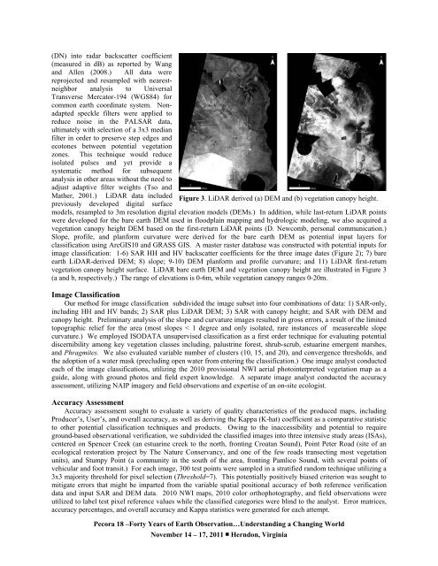This technique would reduce isolated pulses and yet provide a systematic method for subsequent analysis in other areas without the need to adjust adaptive filter weights (Tso and Mather, 2001.) LiDAR data included Figure 3. LiDAR derived (a) DEM and (b) vegetation canopy height. previously developed digital surface models, resampled to 3m resolution digital elevation models (DEMs.) In addition, while last-return LiDAR points were developed for the bare earth DEM used in floodplain mapping and hydrologic modeling, we also acquired a vegetation canopy height DEM based on the first-return LiDAR points (D. Newcomb, personal communication.) Slope, profile, and planform curvature were derived for the bare earth DEM as potential input layers for classification using ArcGIS10 and GRASS GIS. A master raster database was constructed with potential inputs for image classification: 1-6) SAR HH and HV backscatter coefficients for the three image dates (Figure 2); 7) bare earth LiDAR-derived DEM; 8) slope; 9-10) DEM planform and profile curvature; and 11) LiDAR first-return vegetation canopy height surface. LiDAR bare earth DEM and vegetation canopy height are illustrated in Figure 3 (a and b, respectively.) The range of elevations is 0-6m, while vegetation canopy ranges 0-20m. Image Classification Our method for image classification subdivided the image subset into four combinations of data: 1) SAR-only, including HH and HV bands; 2) SAR plus LiDAR DEM; 3) SAR with canopy height; and SAR with DEM and canopy height. Preliminary analysis of the slope and curvature images resulted in gross errors, a result of the limited topographic relief for the area (most slopes < 1 degree and only isolated, rare instances of measureable slope curvature.) We employed ISODATA unsupervised classification as a first order technique for evaluating potential discernibility among key vegetation classes including, palustrine forest, shrub-scrub, estuarine emergent marshes, and Phragmites. We also evaluated variable number of clusters (10, 15, and 20), and convergence thresholds, and the adoption of a water mask (precluding open water from entering the classification.) One image analyst conducted each of the image classifications, utilizing the 2010 provisional NWI aerial photointerpreted vegetation map as a guide, along with ground photos and field expert knowledge. A separate image analyst conducted the accuracy assessment, utilizing NAIP imagery and field observations and expertise of an on-site ecologist. Accuracy Assessment Accuracy assessment sought to evaluate a variety of quality characteristics of the produced maps, including Producer’s, User’s, and overall accuracy, as well as deriving the Kappa (K-hat) coefficient as a comparative statistic to other potential classification techniques and products. Owing to the inaccessibility and potential to require ground-based observational verification, we subdivided the classified images into three intensive study areas (ISAs), centered on Spencer Creek (an estuarine creek to the north, fronting Croatan Sound), Point Peter Road (site of an ecological restoration project by The Nature Conservancy, and one of the few roads transecting most vegetation units), and Stumpy Point (a community in the south of the area, fronting Pamlico Sound, with several points of vehicular and foot transit.) For each image, 300 test points were sampled in a stratified random technique utilizing a 3x3 majority threshold for pixel selection (Threshold=7). This potentially positively biased criterion was sought to mitigate errors that might be imparted from the variable spatial positional accuracy of both reference verification data and input SAR and DEM data. 2010 NWI maps, 2010 color orthophotography, and field observations were utilized to label test pixel reference values while the classified categories were blind to the analyst. Error matrices, accuracy percentages, and overall accuracy and Kappa statistics were generated for each attempt. Pecora 18 –Forty Years of Earth Observation…Understanding a Changing World November 14 – 17, c 2011 ￭ Herndon, Virginia d
Results of the image classification are shown in map form in Figure 4 a-d, depicting the overall mosaic of classes. The SAR-only classification (4a) performed exceptionally well qualitatively with respect to marsh, shrubscrub, and palustrine forest extent and pattern (overall Kappa 0.742). The SAR-only classification yielded an overall accuracy of 80.7% with relatively high user’s accuracy by class (lowest for water with 63.3% while vegetation ranged 71.9% for shrub-scrub to 89.7% for marshes.) The SAR and DEM classification (4b) identified an overabundance of Phragmites, particularly in the Spencer Creek north area (overall Kappa 0.52). The SAR+DEM combination suffered low accuracy with Phragmites (user’s accuracy 42.8%) and marshes (54.4%), likely as a fundamental result of low-lying fringe vegetation being indetermine for interpolated bare earth LiDAR points. SAR and canopy height classification (4c) is visually good, with moderate error in overestimating the extent of Phragmites and open water within Spencer Creek (Kappa = 0.726). SAR+canopy height classified data was superior to SAR+DEM, with better Phragmites results (user’s accuracy 61.1%) and much improved shrub-scrub accuracy (72.8%.) Finally, the SAR imagery with DEM and canopy height included resulted in a good overall upland classification and modest error, visually, among the water and Phragmites. This image (4d) nonetheless identified forest and schrub-scrub discernment very well (Kappa overall 0.744). The overall accuracy for this composite classification using SAR, DEM, and vegetation canopy height was 81.33%, with a surprising disappointment with confusion of RESULTS AND DISCUSSION c d water (60% user’s accuracy). This result is nonetheless very promising, as incorporating a more robust shoreline water mask or infrared-based spectral mask would dramatically reduce this source of confusion (found mianly with commission errors, water being classified as Phragmites.) However, it is equally possible that Phragmites is so dynamic in this area, that is in truth was present at the time imagery was collected. Our field visit with FWS staff and on-site ecologists from The Nature Conservancy (TNC) revealed that the some large areas of Phragmities had just been sprayed by aerial application of herbicides. As a result, the interpretation that open water was not this type vegetation could be in error. Other vegetation was not sprayed, buoying our inference that this initial methodology and combination of data sources could provide a robust and effective method for coastal wetland mapping. CONCLUSIONS a b Figure 4. Results of four image classifications a) SAR-only, b) SAR with DEM, c) SAR with canopy height, and d) SAR with DEM and canopy height. Although results reported in this project are preliminary, we suggest that the literature and convergence of SAR, LiDAR, and geospatial analysis are now mature to the point that heretofore methods for regional wetland inventorying and mapping are highly promising. This project has shown that good accuracy and even high user’s Pecora 18 –Forty Years of Earth Observation…Understanding a Changing World November 14 – 17, 2011 ￭ Herndon, Virginia
Page 1 and 2: ABSTRACT COASTAL WETLAND MAPPING US
Page 3: (pocosins, swamp forests, and pond

coastal wetland mapping using time series sar imagery and ... - asprs

Create successful ePaper yourself

Delete template?

Save as template?