dem users manual - asprs

ABSTRACT
WHAT’S NEW IN THE 2 ND EDITION OF ASPRS’ DEM USERS MANUAL
David F. Maune, Ph.D., CP
Remote Sensing Project Manager
Dewberry & Davis
8401 Arlington Blvd.
Fairfax, VA 22031-4666
dmaune@dewberry.com
The 1 st edition of Digital Elevation Model Technologies and Applications: The DEM Users Manual was published
by ASPRS in 2001. It answered such fundamental questions as “What’s a DEM? What’s a TIN? What’s the
difference between a DEM, DTM and DSM? What is a hydro-enforced DEM? What DEM technology is best for
my needs? How do I know what to ask for to ensure these needs are satisfied? How do I determine that I received
the quality data I paid for? Why can’t we just refer to contour intervals like we used to? How can I understand the
acronyms, terminology, and accuracy standards that seem so confusing?” The 1 st edition answered all such
questions and many more, but the 2 nd edition is much better, not only updating the original chapters, but adding new
chapters, new subjects, and providing sample digital datasets and viewer software on a DVD for users and students
to visualize and “play with” actual data on their own computers ― making this new edition much more valuable as
an academic text book. This paper summarizes the changes in the 2 nd edition, published in 2006.
2 ND EDITION CHAPTERS
DEM technologies have significantly improved over the past five years between publication of the 1 st and 2 nd
editions of the DEM Users Manual. Accuracy standards and guidelines have been published that require DEM users
and producers alike to understand the new terminology and criteria used for quality assessment. The Editor and
authors are convinced that this 2 nd edition will be even more popular than the 1 st edition because the new edition
includes sample digital datasets from each of the technology chapters and from many of the supporting chapters as
well. The following summarizes the major focus of each chapter and major changes between the 1 st and 2 nd editions.
Chapter 1: Introduction
Chapter 1 explains DEM terminology, presents a tutorial on 3-D surface concepts, and provides an introduction
to tides. It is important for DEM users to understand the concepts of mass points and breaklines, triangulated
irregular networks (TINs), how uniformly-spaced DEMs are produced from mass points and breaklines (or from
TINs), and the impact of tides on DEM data in coastal areas. It is also important for DEM users to understand the
differences between digital surface models (DSMs) and digital terrain models (DTMs). Whereas DEMs are often
synonymous with DTMs, the “DEM umbrella” includes bathymetric DEMs and irregularly spaced mass points and
breaklines, TINs, digital contours, and other forms of digital elevation data. This 2 nd edition has improved
information on breaklines, contours, hydrologic enforcement and hydrologic conditioning, and the latest 18.6-year
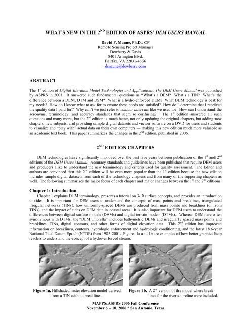
National Tidal Datum Epoch (NTDE) from 1983-2001. Figures 1a and 1b are examples of how better graphics help
readers to understand the concept of a hydro-enforced stream.
Figure 1a. Hillshaded raster elevation model derived
from a TIN without breaklines.
MAPPS/ASPRS 2006 Fall Conference
November 6 – 10, 2006 * San Antonio, Texas
Figure 1b. A 2 nd version of the model where break-
lines for the river shoreline were included.

Chapter 2: Vertical Datums
Chapter 2 explains why there are so many vertical datums used in the United States and why the “official”
North American Vertical Datum of 1988 (NAVD 88) is normally the only one that ought to be used for topographic
applications. It also explains the different tidal datums and how they are used. It is essential that DEM users
understand what the geoid is, the difference between ellipsoid heights and orthometric heights, and reasons why
DEM users should not combine data sets that are referenced to different datums. This is the only chapter with
relatively minor changes between the 1 st and 2 nd editions.
Chapter 3: Accuracy Standards and Guidelines
Chapter 3 explains the National Standard for Spatial Data Accuracy (NSSDA) and compares it with the
traditional National Map Accuracy Standard (NMAS) published in 1947, as well as the ASPRS Standard for Large
Scale Maps published in 1990 (ASPRS 90), both of which were replaced by the NSSDA. Chapter 3 also explains
the relevant standards for hydrographic surveys and the new National Ocean Service “Hydrographic Surveys
Specifications and Deliverables.” This 2 nd edition also includes the new Appendix A, Aerial Mapping and
Surveying, to FEMA’s “Guidelines and Specifications for Flood Hazard Mapping Partners;” the National Digital
Elevation Program (NDEP) “Guidelines for Digital Elevation Data;” and the “ASPRS Guidelines, Vertical Accuracy
Reporting for Lidar Data,” the covers of which are shown in Figures 2a, 2b and 2c. If you don’t know the meanings
of Fundamental Vertical Accuracy (FVA), Consolidated Vertical Accuracy (CVA) and Supplemental Vertical
Accuracy (SVA), Chapter 3 explains what you need to know; and Chapter 12 (DEM Quality Assessment) provides
actual examples of FVA, CVA and SVA statistics and reporting.
Figure 2a. New FEMA Guidelines Figure 2b. New NDEP Guidelines Figure 2c. New ASPRS Guidelines
Chapter 4: National Elevation Dataset
Chapter 4 explains the National Elevation Dataset (NED) which includes the best available standard DEMs
produced and/or distributed nationwide by USGS, comprising the elevation layer of The National Map. NED data
are available to the public at minimal cost, and all users are encouraged to share their data sets with the NED which
places DEM data in the public domain. This 2 nd edition does a better job explaining the three NED resolution layers
available, and how such data can be obtained by the public. Samples of NED data are provided on the DVD
included with this 2 nd edition. Figure 3 helps explain procedures for obtaining NED data.
Chapter 5: Photogrammetry
Chapter 5 has been rewritten to incorporate the latest information from the 5 th Edition of the Manual of
Photogrammetry published by ASPRS. In addition to film cameras, it addresses the latest airborne digital systems
and satellite imagery. For production of digital elevation data, it addresses planning considerations, georeferencing
and aerotriangulation, photogrammetric data collection methods, post processing, quality control, data deliverables,
supporting technologies, calibration procedures, capabilities and limitations compared with competing and/or
complementary technologies, user applications, cost considerations, and technological advancements for the future.
MAPPS/ASPRS 2006 Fall Conference
November 6 – 10, 2006 * San Antonio, Texas

Figure 3. Web-based seamless data distribution system (http://seamless.usgs.gov/) for viewing and downloading of
NED products (left). Large area coverage of NED products available on hard media (right).
Samples of photogrammetric mass points, breaklines and contours are provided on the DVD included with the
manual. Figure 4 provides examples of images that help readers understand a major advantage of softcopy
workstations, i.e., their ability to superimpose all elevation points, and even contours, for review against the actual
ground form, and the ability to selectively review existing, new, and changed data in the same stereoscopic display.
Figure 4. Review of automated terrain extraction by superimposing color-coded crosses to show post accuracies.
MAPPS/ASPRS 2006 Fall Conference
November 6 – 10, 2006 * San Antonio, Texas

Chapter 6: IFSAR
Chapter 6 explains the capabilities and limitations of Interferometric Synthetic Aperture Radar (IFSAR), both
airborne and spaceborne. This technology sees through clouds, is less weather dependent that other technologies,
and acquires elevation data sets of large areas at relatively low costs. It is important that DEM users understand that
elevations derived from x-band IFSAR are initially the elevations of top surfaces (treetops and rooftops) and not the
bare-earth terrain, so if you need DSMs of large areas, this technology may be best for you. DTMs can be produced
from IFSAR DSMs, and a sample IFSAR data set, including an orthorectified radar image, is included on the DVD
that accompanies this 2 nd edition. Figure 5 helps explain how Synthetic Aperture Radar (SAR) works.
Figure 5. The 3-D world is collapsed to 2-D in conventional SAR imaging. After image formation, the radar return
is resolved into an image in range-azimuth coordinates. This figure shows a profile of the terrain at constant
azimuth, with the radar flight track into the page.
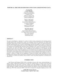
Chapter 7: Topographic and Terrestrial Lidar
Chapter 7 is improved significantly from the 1 st edition, especially in describing different laser systems and how
they work, modern sensors with very high pulse repetition rates, and explaining what a lidar point cloud is. This 2 nd
edition includes entirely new sections on lidargrammetry and ground-based lidar (terrestrial laser scanning) for
which there are nearly 2000 systems in use worldwide today, providing high resolution scanned images of
infrastructure so detailed that every pixel has its own 3-D coordinate. Many different sample lidar datasets are
provided on the DVD included with this 2 nd edition, including topographic and terrestrial lidar and fly-throughs.
Figure 6a shows a point cloud from an airborne lidar sensor, color-coding different lidar returns from the trees and
ground. Figure 6b shows a terrestrial lidar dataset (terrestrial laser scan) what looks like a photograph, except that
every pixel has 3-D coordinates so that as-built measurements are quickly and accurately surveyed.
Figure 6a. Topographic lidar “point clouds,” colorcoded
for 1 st through 4 th returns. Many 1 st returns
(yellow) reach the ground, whereas some of the 3 rd
returns (red) are still in the trees and don’t penetrate.
Figure 6b. High-resolution laser image of a fluid catalytic
cracker (FCC) in a refinery captured with a phased-based
scanner. Each pixel has 3-D x/y/z coordinates.
MAPPS/ASPRS 2006 Fall Conference
November 6 – 10, 2006 * San Antonio, Texas

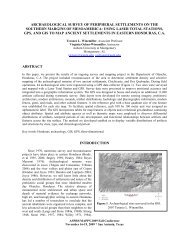
Chapter 8: Airborne Lidar Bathymetry
Chapter 8 documents in detail how this rapidly emerging airborne
lidar bathymetry (ALB) technology is complementary to both sonar and
topographic lidar. ALB systems are able to survey the terrain above and
below the water surface down to a depth limited by the clarity of the water.
ALB is ideal for operations in clear water to depths of 50 meters and near
the land/shore interface for a wide range of near-shore surveying and
engineering applications where sonar may be limited and/or inefficient.
The 2 nd edition includes a considerable number of updates from the 1 st
edition. The enclosed DVD includes a sample ALB dataset. Figure 7 helps
explain how ALB technology works.
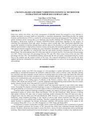
Chapter 9: Sonar
Chapter 9 explains the basic principles of sonar systems and
compares the various kinds of sonars in use today, including vertical
beam, multibeam, interferometric, and side-scan sonar. It compares
these technologies with competing and complementary technologies.
Figure 8. Digital Terrain Model on chart of Eastern Long
Island Sound in 2003, by NOAA Ship Thomas Jefferson.
MAPPS/ASPRS 2006 Fall Conference
November 6 – 10, 2006 * San Antonio, Texas
Figure 7. Schematic diagram of the
effects of scattering on the ALB’s green
lidar beam.
The 2 nd edition has much better graphics than the 1 st
edition of this manual, helping the topographic maping
community to better understand the bathymetric
and hydrographic surveying community, including
similarities and differences. The DVD accompanying
this 2 nd edition includes interesting examples of multibeam
and side-scan sonar and ancillary data.
Figure 8 shows a sample DTM of Eastern Long
Island Sound. It is interesting to note that the
procedures used for QA/QC of bathymetric data are
very similar to procedures used for QA/QC of
topographic data.
Chapter 9 does an excellent job of showing the
similarities and differences in mapping the terrain both
above and below the water’s surface.
Chapter 10: Enabling Technologies
Chapter 10 supports all the technologies described in Chapters 5 through 9 and answers the question of how
such high geopositioning accuracies are achievable. This chapter includes updated sections on precise Global
Positioning System (GPS) positioning on rapidly-moving platforms; GPS-aided inertial navigation systems; direct
georeferencing systems for airborne remote sensing; and motion sensing systems for multibeam sonar bathymetry.
Chapter 11: DEM User Applications
Chapter 11 provides detailed explanations, plus numerous graphic examples, of how digital elevation data are
used in innovative ways for diverse mapping applications; transportation applications (land, air and sea); underwater
and other technical applications; military, commercial and individual applications. The 2 nd edition includes a new
section on coastal mapping applications (shoreline delineation, sea level rise, coastal management, coastal
engineering, and coastal inundation) and a new section on geological applications of digital elevation data. The
DVD accompanying this 2 nd edition includes an interesting 3-D fly-through of a virtual city (Detroit, MI).
Chapter 12: DEM Quality Assessment
Chapter 12 has been largely re-written to address new accuracy standards and guidelines published by FEMA,
NDEP and ASPRS since the 1 st edition. This chapter addresses Quality Assurance/Quality Control (QA/QC) goals
and definitions; quantitative procedures (with example statistics and graphics for a lidar dataset) for assessing digital
elevation data accuracy in accordance with FEMA, NDEP and ASPRS guidelines and accuracy reporting consistent
with NSSDA requirements; different procedures used for qualitative assessments of digital topographic data at
macro and micro levels (with issues and examples); and procedures used by NOAA for quality assessment of digital

hydrographic data. Tables 1 through 4 provide sample dataset calculations of FVA, CVA, SVA and other accuracy
reporting statistics from the quantitative assessment of a lidar dataset.
Table 1 ― DTM Acceptance Criteria from Sample Project Quality Plan
Table 2 ― FVA, CVA and SVA at 95% Confidence Level
Table 3 ― 5% CVA Outliers Larger than 95 th Percentile
Table 4 ― Descriptive Statistics by Land Cover Category
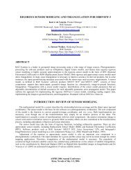
Figure 9 shows errors detected from Dewberry’s independent QA/QC assessments of elevation datasets. Figure
9a illustrates a scan line with high elevations, merged with adjacent scan lines which had the correct elevations; this
tile also was initially classified as bare-earth terrain but it is clear that vegetation still exists within this tile. Figure
9b illustrates a processing error by the vendor where an antenna offset was not applied when reducing the data.
Figures 9c, 9d and 9e show the results of over-smoothing. Figure 9c shows correct processing in the north
(Area A), over-smoothing in the south (Area B). Figure 9d uses cross sections that show a stream in the north and a
pseudo-levee in the south. Figure 9e is an orthophoto that shows the DTM should depict a stream throughout.
MAPPS/ASPRS 2006 Fall Conference
November 6 – 10, 2006 * San Antonio, Texas

Figure 9a. Uncleaned
artifacts (vegetation)
and scan line error.
Figure 9b. Wrong
antenna offset was
used for one tile.
Figure 9c. Area A is
noisy but correct.
Area B is oversmoothed.
Figure 9d. Cross
sections show the
stream becomes a
pseudo-levee.
MAPPS/ASPRS 2006 Fall Conference
November 6 – 10, 2006 * San Antonio, Texas
Figure 9e. Orthophoto
shows reality;
DTM should depict
stream throughout.
Chapter 13: DEM User Requirements
Chapter 13 updates the popular User Requirements Menu with explanations of menu choices, further explains
the new accuracy standards (FVA, CVA and SVA), and provides example Statements of Work (SOWs) for users
who need help in documenting requirements for digital elevation data that also satisfy requirements of Appendix A,
Guidance for Aerial Mapping and Surveying, to FEMA’s “Guidelines and Specifications for Flood Hazard Mapping
Partners.” By popular demand, the User Requirements Menu and two example SOWs are included digitally (as
Word documents) on the DVD accompanying this 2 nd edition.
Chapter 14: Lidar Processing and Software
Chapter 14 is new for the 2 nd edition. It explains lidar software requirements and process flow, to include data
collection, raw data calibration and QA, data production of classified data, and high-level analysis of discrete
features, including automated feature extraction. This chapter peers into the future with regard to lidar software and
processing. Chapter 14 shows many pairs of before/after images to demonstrate the results of various lidar data
processing steps. Figure 10 is one such example where Figure 10a shows what contours would look like before a
double-line stream is hydro-enforced, and Figure 10b shows the contours after hydro-enforcement through the use of
3-D breaklines (polylines).
Figure 10a. Pre-hydro-enforced ground model.
Figure 10b. Hydro-enforced model.
Chapter 15: Sample Elevation Datasets
Chapter 15 is also totally new, and it is the most exciting addition to the 2 nd edition. It explains the viewer
software and sample datasets on the DVD included with the manual. Readers with a computer and DVD reader
should explore the contents of the DVD and view the impressive array of sample data, including: NED data (Chapter
4), photogrammetric data (Chapter 5), IFSAR data (Chapter 6), topographic lidar data (Chapter 7), terrestrial laser

scan data (Chapter 7), bathymetric lidar data (Chapter 8), and sonar data (Chapter 9). It also includes avi video flythroughs
of elevation data from multiple sources, including Pictometry imagery, topographic and terrestrial lidar.
The software and various datasets on the DVD are all explained in this exciting new chapter.
Appendices
Appendix A compiles over 350 acronyms used in the manual, and Appendix B provides nearly 400 definitions.
Thus, if a reader encounters an unfamiliar term and may not recall where that term was defined, look in Appendix B
where hundreds of terms are listed alphabetically, and defined. Appendix C is the color appendix, where all color
Figures are printed.
SUMMARY
It has long been the Editor’s goal that the 2 nd edition not only update the technical content of each chapter, but
also provide a DVD for users to gain some hands-on experience in “playing with” sample elevation datasets. This
DVD will hopefully be instrumental to the development of an exciting academic curriculum in which DEM
technologies and applications are taught to our future industry practitioners. Professors and students will not be
disappointed.
As with the 1 st edition, the new edition has been a voluntary labor of love by the various chapter authors, all of
whom are experts in their particular fields. Their efforts are truly appreciated
The 2 nd edition is dedicated to the memories of two special people who authored chapters in the 1 st and/or 2 nd
editions of the DEM Users Manual and who passed away prior to publication of the 2 nd edition. Ken Osborn was
the principal author of Chapter 4 (National Digital Elevation Program) in the 1 st edition; Ken passed away in March
of 2004. Bob Fowler was the principal author of Chapter 7 (Topographic Lidar) in the 1 st edition, and Chapter 7
(Topographic and Terrestrial Lidar) in the 2 nd edition; Bob passed away in July of 2006. Bob’s last email to the
Editor was when he concurred with the final manuscript of Chapter 7. Ken and Bob both dedicated their careers to
promote greater understanding of DEM technologies and applications and greater access to digital elevation data.
Both were true professionals and friends of the imaging and geospatial information communities that comprise the
“ASPRS family.”
MAPPS/ASPRS 2006 Fall Conference
November 6 – 10, 2006 * San Antonio, Texas