Rigorous Sensor Modeling and Triangulation for OrbView-3 - asprs
Rigorous Sensor Modeling and Triangulation for OrbView-3 - asprs
Rigorous Sensor Modeling and Triangulation for OrbView-3 - asprs

You also want an ePaper? Increase the reach of your titles
YUMPU automatically turns print PDFs into web optimized ePapers that Google loves.
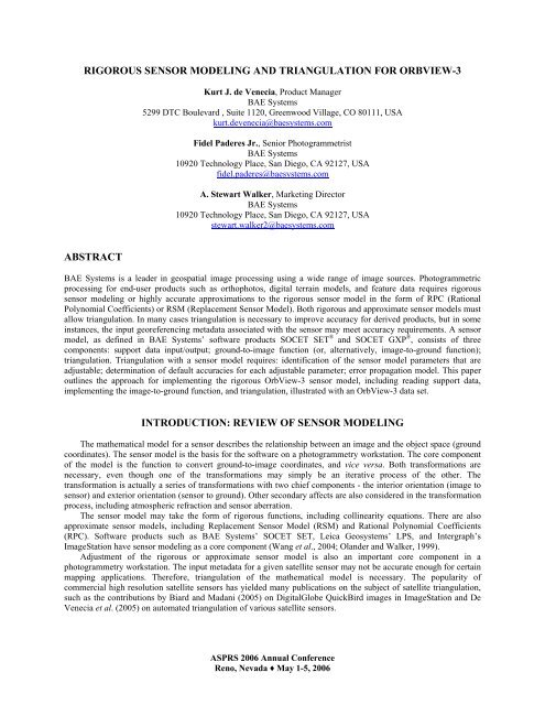
RIGOROUS SENSOR MODELING AND TRIANGULATION FOR ORBVIEW-3<br />
ABSTRACT<br />
Kurt J. de Venecia, Product Manager<br />
BAE Systems<br />
5299 DTC Boulevard , Suite 1120, Greenwood Village, CO 80111, USA<br />
kurt.devenecia@baesystems.com<br />
Fidel Paderes Jr., Senior Photogrammetrist<br />
BAE Systems<br />
10920 Technology Place, San Diego, CA 92127, USA<br />
fidel.paderes@baesystems.com<br />
A. Stewart Walker, Marketing Director<br />
BAE Systems<br />
10920 Technology Place, San Diego, CA 92127, USA<br />
stewart.walker2@baesystems.com<br />
BAE Systems is a leader in geospatial image processing using a wide range of image sources. Photogrammetric<br />
processing <strong>for</strong> end-user products such as orthophotos, digital terrain models, <strong>and</strong> feature data requires rigorous<br />
sensor modeling or highly accurate approximations to the rigorous sensor model in the <strong>for</strong>m of RPC (Rational<br />
Polynomial Coefficients) or RSM (Replacement <strong>Sensor</strong> Model). Both rigorous <strong>and</strong> approximate sensor models must<br />
allow triangulation. In many cases triangulation is necessary to improve accuracy <strong>for</strong> derived products, but in some<br />
instances, the input georeferencing metadata associated with the sensor may meet accuracy requirements. A sensor<br />
model, as defined in BAE Systems’ software products SOCET SET ® <strong>and</strong> SOCET GXP ® , consists of three<br />
components: support data input/output; ground-to-image function (or, alternatively, image-to-ground function);<br />
triangulation. <strong>Triangulation</strong> with a sensor model requires: identification of the sensor model parameters that are<br />
adjustable; determination of default accuracies <strong>for</strong> each adjustable parameter; error propagation model. This paper<br />
outlines the approach <strong>for</strong> implementing the rigorous <strong>OrbView</strong>-3 sensor model, including reading support data,<br />
implementing the image-to-ground function, <strong>and</strong> triangulation, illustrated with an <strong>OrbView</strong>-3 data set.<br />
INTRODUCTION: REVIEW OF SENSOR MODELING<br />
The mathematical model <strong>for</strong> a sensor describes the relationship between an image <strong>and</strong> the object space (ground<br />
coordinates). The sensor model is the basis <strong>for</strong> the software on a photogrammetry workstation. The core component<br />
of the model is the function to convert ground-to-image coordinates, <strong>and</strong> vice versa. Both trans<strong>for</strong>mations are<br />
necessary, even though one of the trans<strong>for</strong>mations may simply be an iterative process of the other. The<br />
trans<strong>for</strong>mation is actually a series of trans<strong>for</strong>mations with two chief components - the interior orientation (image to<br />
sensor) <strong>and</strong> exterior orientation (sensor to ground). Other secondary affects are also considered in the trans<strong>for</strong>mation<br />
process, including atmospheric refraction <strong>and</strong> sensor aberration.<br />
The sensor model may take the <strong>for</strong>m of rigorous functions, including collinearity equations. There are also<br />
approximate sensor models, including Replacement <strong>Sensor</strong> Model (RSM) <strong>and</strong> Rational Polynomial Coefficients<br />
(RPC). Software products such as BAE Systems’ SOCET SET, Leica Geosystems’ LPS, <strong>and</strong> Intergraph’s<br />
ImageStation have sensor modeling as a core component (Wang et al., 2004; Ol<strong>and</strong>er <strong>and</strong> Walker, 1999).<br />
Adjustment of the rigorous or approximate sensor model is also an important core component in a<br />
photogrammetry workstation. The input metadata <strong>for</strong> a given satellite sensor may not be accurate enough <strong>for</strong> certain<br />
mapping applications. There<strong>for</strong>e, triangulation of the mathematical model is necessary. The popularity of<br />
commercial high resolution satellite sensors has yielded many publications on the subject of satellite triangulation,<br />
such as the contributions by Biard <strong>and</strong> Madani (2005) on DigitalGlobe QuickBird images in ImageStation <strong>and</strong> De<br />
Venecia et al. (2005) on automated triangulation of various satellite sensors.<br />
ASPRS 2006 Annual Conference<br />
Reno, Nevada ♦ May 1-5, 2006
Replacing the rigorous sensor model with an RPC approximation is popular mainly <strong>for</strong> its simplicity. The<br />
January 2003 issue of Photogrammetric Engineering & Remote Sensing contained four papers discussing RPC <strong>and</strong><br />
RPC triangulation. An RPC model, especially when embedded in st<strong>and</strong>ard imagery <strong>for</strong>mats such as NITF, allows<br />
software developers to implement the RPC model once <strong>for</strong> any sensor using the st<strong>and</strong>ardized <strong>for</strong>mat. Un<strong>for</strong>tunately<br />
RPC modeling does not lend itself to long image segments where high frequency corrections cannot be accounted<br />
<strong>for</strong> in the st<strong>and</strong>alone RPC model. The Replacement <strong>Sensor</strong> Model (McGlone, 2004) is a promising extension to the<br />
RPC model. But, until the RSM is fully accepted by the end-user, data provider, <strong>and</strong> software developer<br />
communities, rigorous models will continue to be used <strong>for</strong> complex modeling of airborne <strong>and</strong> satellite sensors.<br />
ORBVIEW-3 SENSOR MODELING AND ASSOCIATED SUPPORT DATA<br />
The <strong>OrbView</strong>-3 satellite carries a linear array pushbroom sensor, providing one meter panchromatic <strong>and</strong> four<br />
meter multispectral imagery. GeoEye sells imagery <strong>and</strong> metadata at varying levels of processing. There are currently<br />
eight <strong>OrbView</strong>-3 products, from BASIC imagery to Orthorectified products (ORTHO). This paper focuses on<br />
<strong>OrbView</strong>-3 BASIC Enhanced Panchromatic Imagery, which includes enhanced telemetry metadata.<br />
Cooperation between the data provider <strong>and</strong> the photogrammetry software supplier is essential to underst<strong>and</strong>ing<br />
<strong>and</strong> implementing the rigorous sensor model <strong>for</strong> a specific sensor. In the case of <strong>OrbView</strong>-3 imagery, agreements<br />
were signed between BAE Systems <strong>and</strong> ORBIMAGE (now GeoEye), then technical material <strong>and</strong> sample imagery<br />
were provided by ORBIMAGE. <strong>OrbView</strong>-3 BASIC Enhanced Imagery including enhanced telemetry data was sent<br />
to BAE Systems along with ground control <strong>and</strong> documentation describing the imagery <strong>and</strong> metadata. Clearly,<br />
cooperation in both business <strong>and</strong> technical aspects is mutually beneficial <strong>for</strong> the data provider (GeoEye) <strong>and</strong> data<br />
user (BAE Systems) – GeoEye wishes to sell imagery products <strong>and</strong> BAE Systems wishes to sell image exploitation<br />
software to mapping <strong>and</strong> intelligence agencies <strong>and</strong> commercial companies.<br />
Support data includes in<strong>for</strong>mation such as sensor location, velocity, orientation angles, focal length, time of<br />
acquisition, <strong>and</strong> camera calibration data. Support data are often supplied as auxiliary files to the raw imagery. In the<br />
past imagery <strong>and</strong> metadata were typically re<strong>for</strong>matted in the photogrammetry workstation into a common <strong>for</strong>mat <strong>for</strong><br />
convenient use by the image processing software solutions such as SOCET SET, but today the image providers are<br />
typically delivering their imagery in common <strong>for</strong>mats such as NITF <strong>and</strong> TIFF. There<strong>for</strong>e, the imagery is often used<br />
directly <strong>for</strong> photogrammetric processing in the software. The associated image metadata is normally stored in a<br />
binary or ASCII <strong>for</strong>mat. Documentation provided by ORBIMAGE details the metadata definition <strong>and</strong> <strong>for</strong>mat. The<br />
SOCET SET <strong>and</strong> SOCET GXP software products use the <strong>OrbView</strong>-3 imagery <strong>and</strong> metadata directly without the<br />
need to re<strong>for</strong>mat either input data source. Since triangulation is typically required by end-users of the<br />
photogrammetry software, a solution providing updated sensor parameters must be provided. In the case of SOCET<br />
SET <strong>and</strong> SOCET GXP, the updated (triangulated) sensor parameters are stored in a separate ASCII support file.<br />
The sensor model converts ground space locations to image space locations, or vice versa. The ground space<br />
coordinates are in the <strong>for</strong>m of Earth-Centered-Earth-Fixed (ECEF) coordinates in meters. The image coordinates are<br />
sub-pixel line <strong>and</strong> sample coordinates. The trans<strong>for</strong>mations are used in nearly every photogrammetric process, from<br />
simply moving the cursor on an image to creating products such as orthophotos. The <strong>OrbView</strong>-3 sensor model<br />
documentation provided by ORBIMAGE outlines the image-to-ground trans<strong>for</strong>mation. There<strong>for</strong>e, the direct imageto-ground<br />
trans<strong>for</strong>mation was implemented in SOCET SET <strong>and</strong> SOCET GXP with the ground-to-image<br />
implemented as an iterative computation of the image-to-ground. The <strong>OrbView</strong>-3 documentation outlines the<br />
projective image-to-ground trans<strong>for</strong>mation as<br />
where<br />
G 1 A k<br />
O<br />
= A + M a<br />
(1)<br />
G<br />
A is the unknown object space coordinate triplet in the ECEF WGS84 coordinate system in meters<br />
O<br />
A is the instantaneous sensor position triplet in the ECEF WGS84 coordinate system in meters<br />
interpolated from the ephemeris metadata<br />
k is a scalar<br />
M is the 3x3 image-to-ground rotation matrix based on instantaneous attitude in<strong>for</strong>mation in the <strong>for</strong>m of<br />
quaternion values from the attitude metadata<br />
ASPRS 2006 Annual Conference<br />
Reno, Nevada ♦ May 1-5, 2006
a is the imaging vector consisting of image space coordinates <strong>and</strong> focal length trans<strong>for</strong>med to meters<br />
using interior orientation coefficients provided in the <strong>OrbView</strong>-3 metadata.<br />
Implementation in software of a satellite sensor model including triangulation is typically an 8-10 week task,<br />
encompassing design, code, <strong>and</strong> test prior to release in a specified software version. Technical cooperation <strong>and</strong><br />
communication between BAE Systems <strong>and</strong> ORBIMAGE resulted in a smooth development cycle. Complete details<br />
regarding the trans<strong>for</strong>mation (equation 1) were provided by ORBIMAGE <strong>and</strong> it is provided here to allow discussion<br />
of the triangulation <strong>for</strong> <strong>OrbView</strong>-3 implemented in SOCET SET. In addition to the direct projective trans<strong>for</strong>mation<br />
model in equation 1 are secondary affects such as atmospheric correction <strong>and</strong> vehicle aberration.<br />
ORBVIEW-3 SENSOR MODEL TRIANGULATION<br />
The triangulation function provides a mechanism <strong>for</strong> updating the interior <strong>and</strong> exterior orientation elements <strong>for</strong><br />
the <strong>OrbView</strong>-3 sensor’s metadata. The multi-sensor triangulation function in SOCET SET requires:<br />
Identification of which parameters of the sensor model are adjustable<br />
Determination of whether the adjustment provides corrections or absolute values<br />
Determination of the names <strong>for</strong> the adjustable parameters <strong>for</strong> a logical user interface<br />
Determination of the default accuracies <strong>for</strong> each adjustable parameter<br />
Determination of the perturbation values <strong>for</strong> the parameters, to compute partial derivatives numerically.<br />
Based on the <strong>OrbView</strong>-3 documentation <strong>and</strong> engineering experience with satellite pushbroom sensors, 23<br />
parameters were chosen <strong>for</strong> adjustment. All adjustable parameters of the <strong>OrbView</strong>-3 sensor model within SOCET<br />
SET are corrections to the actual values provided in the image metadata. The 23 <strong>OrbView</strong>-3 sensor model<br />
parameters consist of five corrections <strong>for</strong> interior orientation <strong>and</strong> 18 corrections <strong>for</strong> the six elements of exterior<br />
orientation. The five interior orientation elements are non-time dependent, while the six exterior orientation<br />
elements are quadratic functions of acquisition time. The model <strong>and</strong> triangulation assume the time duration of<br />
acquisition is relatively short. If larger segments are to be triangulated, then additional parameters may need to be<br />
included. The additional parameters used in other satellite pushbroom sensor models in SOCET SET include an<br />
along-track correction to the attitude <strong>and</strong> position in the <strong>for</strong>m of a finite element correction profile. Details of the<br />
five triangulated parameters <strong>for</strong> interior orientation are<br />
where<br />
⎡ x<br />
⎢<br />
= ⎢ y<br />
⎢<br />
⎣ f<br />
⎤ ⎡ x<br />
⎥ ⎢<br />
⎥ = ⎢y<br />
⎥ ⎢<br />
⎦ ⎣<br />
δ<br />
+ x ⎤ 1 S<br />
δ ⎥<br />
+ y S⎥<br />
δ<br />
f ⎥<br />
⎦<br />
δ δ<br />
0<br />
δ<br />
a<br />
δ<br />
δ<br />
δ<br />
0 1<br />
δ<br />
a is the correction to the imaging vector in meters<br />
δ δ<br />
δ<br />
x , y , <strong>and</strong> f are the corrections to the image x, y coordinates <strong>and</strong> focal length, respectively<br />
δ δ<br />
x0<br />
<strong>and</strong> y0<br />
are the triangulated offset corrections to the image x, y coordinates<br />
δ δ<br />
x1<br />
<strong>and</strong> y1<br />
are the triangulated linear corrections to the image x, y coordinates<br />
S is the input sample coordinate <strong>for</strong> the image-to-ground trans<strong>for</strong>mation.<br />
The nine triangulated parameters <strong>for</strong> exterior orientation attitude corrections are<br />
ASPRS 2006 Annual Conference<br />
Reno, Nevada ♦ May 1-5, 2006<br />
(2)
where<br />
where<br />
δ δ<br />
ω , ϕ , <strong>and</strong> κ<br />
δ<br />
δ δ δ<br />
δ 2<br />
⎡ω<br />
⎤ ⎡ω<br />
⎤ ⎡ ⎤ ⎡ ⎤<br />
0 ω1<br />
TC<br />
ω2TC<br />
⎢ δ ⎥ ⎢ δ ⎥ ⎢ δ ⎥ ⎢ δ 2 ⎥<br />
⎢ϕ<br />
⎥ = ⎢ϕ0<br />
⎥ + ⎢ϕ1<br />
TC<br />
⎥ + ⎢ϕ2<br />
TC<br />
⎥<br />
⎢ δ ⎥ ⎢ δ ⎥ ⎢ δ ⎥ ⎢ δ 2 ⎥<br />
⎣κ<br />
⎦ ⎣κ0<br />
⎦ ⎣κ1<br />
TC<br />
⎦ ⎣κ<br />
2TC<br />
⎦<br />
are the corrections to the image-to-ground Euler orientation angles, omega, phi, <strong>and</strong><br />
kappa, respectively, whose initial values are assumed zeros<br />
δ δ δ<br />
ω0 , ϕ0<br />
, <strong>and</strong> κ0<br />
are the triangulated offset correction values <strong>for</strong> omega, phi, <strong>and</strong> kappa, respectively<br />
δ δ δ<br />
ω1 , ϕ1<br />
, <strong>and</strong> κ1<br />
are the triangulated linear (velocity) correction values <strong>for</strong> omega, phi, <strong>and</strong> kappa,<br />
respectively<br />
δ δ δ<br />
ω2 , ϕ2<br />
, <strong>and</strong> κ2<br />
are the triangulated non-linear (acceleration) correction values <strong>for</strong> omega, phi, <strong>and</strong><br />
kappa, respectively<br />
TC is the time at the given input line coordinate with origin at image center.<br />
The exterior orientation positional corrections are<br />
A<br />
δ<br />
⎡X<br />
⎢<br />
= ⎢Y<br />
⎢<br />
⎣ Z<br />
δ<br />
δ<br />
δ<br />
δ δ<br />
δ 2<br />
⎤ ⎡X<br />
⎤ ⎡ ⎤ ⎡ ⎤<br />
0 X1<br />
Tc<br />
X 2Tc<br />
⎥ ⎢ δ ⎥ ⎢ δ ⎥ ⎢ δ 2 ⎥<br />
⎥ = ⎢Y0<br />
⎥ + ⎢Y1<br />
Tc<br />
⎥ + ⎢Y2<br />
Tc<br />
⎥<br />
⎥ ⎢ δ ⎥ ⎢ δ ⎥ ⎢ δ 2 ⎥<br />
⎦ ⎣ Z0<br />
⎦ ⎣ Z1<br />
Tc<br />
⎦ ⎣ Z2<br />
Tc<br />
⎦<br />
δ<br />
A is the correction <strong>for</strong> the sensor position vector in ECEF WGS84 meters<br />
δ δ<br />
δ<br />
X , Y , <strong>and</strong> Z<br />
are corrections to the sensor position in ECEF WGS84 meters, respectively<br />
δ δ<br />
δ<br />
X 0 , Y0<br />
, <strong>and</strong> Z0<br />
are the triangulated offset correction values <strong>for</strong> the sensor position<br />
δ δ<br />
δ<br />
X1<br />
, Y1<br />
, <strong>and</strong> Z1<br />
are the triangulated linear (velocity) correction values <strong>for</strong> the sensor position<br />
δ δ<br />
δ<br />
X 2 , Y2<br />
, <strong>and</strong> Z2<br />
are the triangulated non-linear (acceleration) correction values <strong>for</strong> the sensor position<br />
T C is the time at the given input line coordinate with origin at image center.<br />
Equation 1 can be updated based on the triangulation components outlined in equations 2-4. The new image-toground<br />
function is<br />
G O δ 1<br />
A = A + A + k<br />
M<br />
δ ( a + a )<br />
δ<br />
where M is the 3x3 correction rotation matrix defined by image-to-ground Euler angle corrections<br />
δ δ δ<br />
ω , ϕ , <strong>and</strong> κ from equation 3. The M rotation matrix is <strong>for</strong>med from the quaternion values interpolated based<br />
on time (T ) from the attitude metadata. All other parameters are defined in equations 1-4 above.<br />
ASPRS 2006 Annual Conference<br />
Reno, Nevada ♦ May 1-5, 2006<br />
δ<br />
M<br />
(3)<br />
(4)<br />
(5)
ORBVIEW-3 MULTI-SENSOR TRIANGULATION EXAMPLE<br />
Tests of the <strong>OrbView</strong>-3 sensor model <strong>and</strong> triangulation were per<strong>for</strong>med with the imagery, metadata <strong>and</strong> ground<br />
control points provided by ORBIMAGE during the development phase of the sensor model. Two additional<br />
<strong>OrbView</strong>-3 BASIC Enhanced Imagery scenes with enhanced telemetry were subsequently sent to BAE Systems <strong>for</strong><br />
testing the SOCET SET Multi-<strong>Sensor</strong> <strong>Triangulation</strong> (MST) with overlapping imagery from two additional satellite<br />
sensors – IKONOS RPC <strong>and</strong> QuickBird Basic. The dataset used <strong>for</strong> testing consists of six images from three<br />
different sensors taken over Denver, Colorado USA. An overview of the imagery is provided in Table 1.<br />
Table 1. Overview of the six images used <strong>for</strong> triangulation. The six images were acquired from three different<br />
satellites <strong>and</strong> are modeled by three different sensor models in SOCET SET <strong>and</strong> SOCET GXP.<br />
Imagery<br />
IKONOS (2)<br />
Pan 11-bit/b<strong>and</strong> NITF<br />
Stereo Epipolar RPC <strong>Sensor</strong> Model<br />
Thumbnail Footprints<br />
Ground Sample Dist: 1.0 m<br />
Size (lines x samples): 12252x9843<br />
12252x9843<br />
The two images overlap by 100% <strong>and</strong> are<br />
same pass stereo.<br />
QuickBird (2)<br />
Basic Panchromatic 11-bit TIFF<br />
Physical Pushbroom <strong>Sensor</strong> Model<br />
Ground Sample Distance: 0.7 m<br />
Size (lines x samples): 28592x27552<br />
29888x27552<br />
<strong>OrbView</strong>-3 (2)<br />
Basic Panchromatic 11-bit/pixel TIFF<br />
Physical Pushbroom <strong>Sensor</strong> Model<br />
Ground Sample Distance: 0.98 m<br />
Size (lines x samples): 34406x8016<br />
30879x8016<br />
Some cloud cover on the bottom of one<br />
of the images.<br />
SOCET SET MST requires proper default settings <strong>for</strong> the accuracy of the parameters of the input imagery.<br />
These are determined at the time the sensor model is implemented. The accuracies <strong>and</strong> adjusted parameters <strong>for</strong> each<br />
image <strong>and</strong>/or sensor can be changed by the operator within the MST application, but <strong>for</strong> an automated process the<br />
accuracies <strong>and</strong> parameters should be well defined. With proper accuracies <strong>for</strong> the selected parameters, the<br />
ASPRS 2006 Annual Conference<br />
Reno, Nevada ♦ May 1-5, 2006
triangulation can be per<strong>for</strong>med on multiple images <strong>and</strong> sensors using tie points only in the fully weighted least<br />
squares bundle adjustment.<br />
Automatic Point Measurement (APM) provides a mechanism to measure tie points automatically between<br />
overlapping imagery regardless of the image <strong>for</strong>mat or sensor type. APM was per<strong>for</strong>med on the six input images<br />
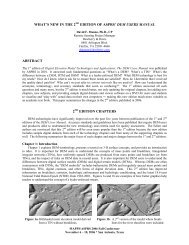
using a regular grid tie point pattern. The results <strong>for</strong> the tie point distribution <strong>and</strong> number are displayed in Figure 1.<br />
Figure 1. Tie points after SOCET SET APM <strong>and</strong> MST bundle adjustment with blunder detection. The zero ray tie<br />
points were eliminated as part of blunder detection. The maximum number of overlaps from the input imagery is<br />
five. The three five ray points can be seen in the center of the block, which is also the location of the high resolution<br />
orthophoto used to check the absolute accuracy of the block. The check point orthophoto footprint is shown in black.<br />
An important element in the MST fully weighted least squares bundle adjustment is automatic blunder<br />
detection. Enabling this feature detected <strong>and</strong> deleted 42 points from the six image block: these points are depicted in<br />
red in Figure 1. The resultant RMS of the tie points was just under one pixel. It was determined after analysis of the<br />
graphical display of residuals with associated imagery that the long <strong>OrbView</strong>-3 image strips were being constrained<br />
too tightly based on the a priori accuracy estimates <strong>for</strong> the parameters. There<strong>for</strong>e, the accuracy values <strong>for</strong> the<br />
exterior orientation elements <strong>for</strong> the offset <strong>and</strong> linear terms in equations 3 <strong>and</strong> 4 were increased (loosened) to allow<br />
more adjustment <strong>for</strong> these parameters. The resultant RMS <strong>for</strong> pixel space residuals decreased to 0.86 pixels.<br />
Check points were used to determine the absolute accuracy of the six image multi-sensor triangulation. The<br />
check points were derived from a high resolution orthomosaic that was created from digital frame images <strong>and</strong><br />
LIDAR courtesy of Merrick <strong>and</strong> Company. The high resolution orthomosaic has a ground sample distance of 15<br />
centimeters. The check points were manually measured in the satellite imagery. Each check point fell within the<br />
five-image overlap region as shown in Figure 1. Table 2 outlines the horizontal check point differences.<br />
ASPRS 2006 Annual Conference<br />
Reno, Nevada ♦ May 1-5, 2006<br />
Rays Color Tie<br />
Points<br />
0 42<br />
2 102<br />
3 27<br />
4 14<br />
5 3
Table 2. Horizontal check points derived from a 15 cm orthomosaic, which was created from digital frame<br />
imagery <strong>and</strong> an associated LIDAR surface. Each check point fell within the five-image overlap region (see<br />
Figure 1). MST computed the difference between the check point original coordinates <strong>and</strong> the multi-ray<br />
intersected check point coordinates.<br />
Check Point<br />
Original<br />
Coordinates<br />
Check Point<br />
Computed<br />
Coordinates<br />
ASPRS 2006 Annual Conference<br />
Reno, Nevada ♦ May 1-5, 2006<br />
Check Point<br />
Differences<br />
(meters)<br />
Point Longitude/<br />
Number Latitude<br />
1 Longitude -104:59:19.917 -104:59:19.983 1.572<br />
Latitude +39:44:23.581 +39:44:23.498 2.552<br />
2 Longitude -104:59:34.602 -104:59:34.568 -0.795<br />
Latitude +39:44:24.226 +39:44:24.110 3.576<br />
3 Longitude -104:59:55.875 -104:59:55.867 -0.198<br />
Latitude +39:44:29.071 +39:44:28.993 2.404<br />
4 Longitude -104:59:39.400 -104:59:39.400 -0.010<br />
Latitude +39:44:41.672 +39:44:41.661 0.347<br />
5 Longitude -104:59:18.934 -104:59:18.884 -1.183<br />
Latitude +39:44:52.649 +39:44:52.634 0.481<br />
6 Longitude -104:59:10.123 -104:59:10.135 0.286<br />
Latitude +39:44:59.406 +39:44:59.339 2.070<br />
7 Longitude -104:58:56.380 -104:58:56.377 -0.073<br />
Latitude +39:44:51.083 +39:44:51.048 1.069<br />
8 Longitude -104:58:56.492 -104:58:56.429 -1.516<br />
Latitude +39:44:35.699 +39:44:35.685 0.449<br />
9 Longitude -104:58:52.050 -104:58:52.023 -0.637<br />
Latitude +39:44:23.994 +39:44:23.912 2.524<br />
10 Longitude -104:59:05.486 -104:59:05.518 0.774<br />
Latitude +39:44:35.659 +39:44:35.647 0.379<br />
11 Longitude -104:59:26.834 -104:59:26.857 0.535<br />
Latitude +39:44:32.052 +39:44:31.993 1.837<br />
12 Longitude -104:59:16.928 -104:59:16.955 0.637<br />
Latitude<br />
RMS<br />
+39:44:44.524 +39:44:44.489 1.091<br />
Total Longitude<br />
RMS<br />
0.848<br />
Latitude 1.874<br />
CONCLUSION<br />
Development of a rigorous sensor model <strong>for</strong> a photogrammetric software solution requires cooperation between<br />
data provider <strong>and</strong> software supplier. Underst<strong>and</strong>ing the physical parameters of the sensor is important in determining<br />
how parameters will be adjusted in the triangulation process.<br />
An RPC model, especially when embedded in st<strong>and</strong>ard imagery <strong>for</strong>mats such as NITF, allows developers to<br />
implement the RPC model once. Only testing is required when data providers launch <strong>and</strong> deliver subsequent image<br />
products in these st<strong>and</strong>ard <strong>for</strong>mats. Un<strong>for</strong>tunately RPC modeling does not lend itself to long image segments, where<br />
high frequency corrections cannot be accounted <strong>for</strong> in the RPC model. Until a replacement sensor model is<br />
embraced by data providers, photogrammetry software suppliers, <strong>and</strong> end-users, the rigorous sensor model will<br />
continue to be the core component of a photogrammetry software solution.
ACKNOWLEDGEMENTS<br />
The authors would like to thank the data providers: ORBIMAGE <strong>and</strong> Space Imaging (now GeoEye);<br />
DigitalGlobe; <strong>and</strong> Merrick <strong>and</strong> Company.<br />
REFERENCES<br />
Biard, J., <strong>and</strong> M. Madani (2005). H<strong>and</strong>ling of DigitalGlobe QuickBird images in Intergraph ImageStation. In:<br />
Conference Proceedings, 2005 ASPRS Annual Conference, March 7-11, 2005, Baltimore, Maryl<strong>and</strong>,<br />
unpaginated CD-ROM, 7 pp.<br />
De Venecia, K., R. Racine, <strong>and</strong> A.S. Walker (2005). End-to-end photogrammetry <strong>for</strong> non-professional<br />
photogrammetrists. In: Conference Proceedings, 2005 ASPRS Annual Conference, March 7-11, 2005,<br />
Baltimore, Maryl<strong>and</strong>, unpaginated CD-ROM, 10 pp.<br />
Fraser, C. S. <strong>and</strong> H. B. Hanley (2003). Bias compensation in rational functions <strong>for</strong> IKONOS satellite imagery.<br />
Photogrammetric Engineering & Remote Sensing, 69(1):53-57.<br />
Grodecki, J., <strong>and</strong> G. Dial (2003). Block adjustment of high-resolution satellite images described by rational<br />
polynomials. Photogrammetric Engineering & Remote Sensing, 69(1):59-68.<br />
Kaichang D., M. Ruijin, <strong>and</strong> Rong Xing Li (2003). Rational functions <strong>and</strong> potential <strong>for</strong> rigorous sensor model<br />
recovery. Photogrammetric Engineering & Remote Sensing, 69(1):33-41.<br />
McGlone, J.C. (ed.) (2004). Manual of Photogrammetry, Fifth Edition. American Society <strong>for</strong> Photogrammetry <strong>and</strong><br />
Remote Sensing, Bethesda, Maryl<strong>and</strong>, pp. 887-943.<br />
Ol<strong>and</strong>er, N. F., <strong>and</strong> A.S. Walker (1998). <strong>Modeling</strong> spaceborne <strong>and</strong> airborne sensors in software. In: International<br />
Archives of Photogrammetry <strong>and</strong> Remote Sensing. Cambridge-Engl<strong>and</strong>. Vol. 32 Part 2, pp. 223-228.<br />
Toutin, T. (2003). Error tracking in IKONOS geometric processing using a 3D parametric model. Photogrammetric<br />
Engineering & Remote Sensing, 69(1):43-51.<br />
Wang, Y., Y. Xinghe, M. Stojic, <strong>and</strong> B. Skelton (2004). Toward higher automation <strong>and</strong> flexibility in commercial<br />
digital photogrammetric systems. In: International Archives of Photogrammetry <strong>and</strong> Remote Sensing.<br />
Istanbul-Turkey. Vol. 35 Part B2, pp 838-840.<br />
SOCET SET® <strong>and</strong> SOCET GXP® are registered trademarks of BAE Systems National Security Solutions Inc.<br />
All rights reserved.<br />
ASPRS 2006 Annual Conference<br />
Reno, Nevada ♦ May 1-5, 2006