3.5 Space Curves in Matlab
3.5 Space Curves in Matlab
3.5 Space Curves in Matlab

You also want an ePaper? Increase the reach of your titles
YUMPU automatically turns print PDFs into web optimized ePapers that Google loves.
<strong>3.5</strong> <strong>Space</strong> <strong>Curves</strong> <strong>in</strong> <strong>Matlab</strong><br />
Section <strong>3.5</strong> <strong>Space</strong> <strong>Curves</strong> <strong>in</strong> <strong>Matlab</strong> 239<br />
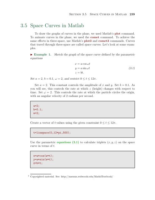
To draw the graphs of curves <strong>in</strong> the plane, we used <strong>Matlab</strong>’s plot command.<br />
To animate curves <strong>in</strong> the plane, we used the comet command. To achieve the<br />
same effects <strong>in</strong> three-space, use <strong>Matlab</strong>’s plot3 and comet3 commands. <strong>Curves</strong><br />
that travel through three-space are called space curves. Let’s look at some examples.<br />
◮ Example 1. Sketch the graph of the space curve def<strong>in</strong>ed by the parametric<br />
equations<br />
x = a cos ωt<br />
y = a s<strong>in</strong> ωt<br />
z = bt.<br />
Set a = 2, b = 0.1, ω = 2, and restrict 0 ≤ t ≤ 12π.<br />
(3.1)<br />
Set a = 2. This constant controls the amplitude of x and y. Set b = 0.1. As<br />
you will see, this controls the rate at which z (height) changes with respect to<br />
time. Set ω = 2. This controls the rate at which the particle circles the orig<strong>in</strong>,<br />
with an angular velocity of 2 radians per second.<br />
a=2;<br />
b=0.1;<br />
w=2;<br />
Create a vector of t-values us<strong>in</strong>g the given constra<strong>in</strong>t 0 ≤ t ≤ 12π.<br />
t=l<strong>in</strong>space(0,12*pi,500);<br />
Use the parametric equations (3.1) to calculate triplets (x, y, z) on the space<br />
curve <strong>in</strong> terms of t.<br />
x=a*cos(w*t);<br />
y=a*s<strong>in</strong>(w*t);<br />
z=b*t;<br />
1<br />
Copyrighted material. See: http://msenux.redwoods.edu/Math4Textbook/
240 Chapter 3 Plott<strong>in</strong>g <strong>in</strong> <strong>Matlab</strong><br />
To get a sense of the motion, use the comet3 command.<br />
comet3(x,y,z)<br />
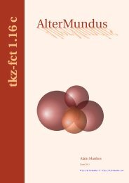
To provide a f<strong>in</strong>ished plot, use <strong>Matlab</strong>’s plot3 command, then add axes labels<br />
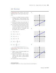
and a title. The follow<strong>in</strong>g commands will produce the helix shown <strong>in</strong> Figure 3.1<br />
plot3(x,y,z)<br />
xlabel(’x-axis’)<br />
ylabel(’y-axis’)<br />
zlabel(’z-axis’)<br />
title(’x = 2 cos(t), y = 2 s<strong>in</strong>(t), z = 0.1t.’)<br />
Figure 3.1. The space curve determ<strong>in</strong>e by the parametric<br />
equations (3.1) is called a helix.<br />
Let’s look at another example.<br />
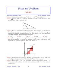
◮ Example 2. Suppose that a ship travels from the south pole to the north<br />
pole keep<strong>in</strong>g a fixed angle to all meridians. Then the path traveled is described<br />
by the parametric equations
Section <strong>3.5</strong> <strong>Space</strong> <strong>Curves</strong> <strong>in</strong> <strong>Matlab</strong> 241<br />
x =<br />
y =<br />
z = −<br />
cos t<br />
√ 1 + α 2 t 2<br />
s<strong>in</strong> t<br />
√ 1 + α 2 t 2<br />
Set α = 0.2 and restrict −12π ≤ t ≤ 12π.<br />
αt<br />
√ 1 + α 2 t 2 .<br />
(3.2)<br />
Set α = 0.2 and create a vector of t-values subject to the constra<strong>in</strong>t −12π ≤<br />
t ≤ 12π.<br />
alpha=0.2;<br />
t=l<strong>in</strong>space(-12*pi,12*pi,500);<br />
Use the parametric equations (3.2) to compute the positions (x, y, z) on the<br />
spherical spiral as a function of time t.<br />
x=cos(t)./sqrt(1+alpha^2*t.^2);<br />
y=s<strong>in</strong>(t)./sqrt(1+alpha^2*t.^2);<br />
z=alpha*t./sqrt(1+alpha^2*t.^2);<br />
Use comet3 to animate the motion, then follow this with <strong>Matlab</strong>’s plot3 command.<br />
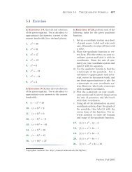
This will produce the spherical spiral shown <strong>in</strong> Figure 3.2.<br />
plot3(x,y,z)<br />
Handle Graphics<br />
Many space curves are closely related with one or another particular class of<br />
surfaces. In the case of the spherical spiral, one would <strong>in</strong>tuit a close relationship<br />
with a sphere. So, let’s draw a sphere of appropriate radius, then superimpose<br />
the spherical spiral of Example 2.<br />
In the section on Parametric Surfaces, we saw the parametric equations of a<br />
sphere of radius r, which we repeat here for convenience.
242 Chapter 3 Plott<strong>in</strong>g <strong>in</strong> <strong>Matlab</strong><br />
Figure 3.2. The path taken by the ship is an example of a<br />
spherical spiral.<br />
x = r s<strong>in</strong> φ cos θ<br />
y = r s<strong>in</strong> φ s<strong>in</strong> θ<br />
z = r cos φ<br />
Set r = 1 and create a grid of (φ, θ) pairs, where 0 ≤ φ ≤ π and 0 ≤ θ ≤ 2π.<br />
r=1;<br />
phi=l<strong>in</strong>space(0,pi,30);<br />
theta=l<strong>in</strong>space(0,2*pi,40);<br />
[phi,theta]=meshgrid(phi,theta);<br />
(3.3)<br />
Use the parametric equations (3.3) to compute each po<strong>in</strong>t (x, y, z) on the surface<br />
of the sphere as a function of each grid pair (φ, θ).<br />
x=r*s<strong>in</strong>(phi).*cos(theta);<br />
y=r*s<strong>in</strong>(phi).*s<strong>in</strong>(theta);<br />
z=r*cos(phi);<br />
Now, plot the sphere with the mesh command.
mhndl=mesh(x,y,z)<br />
Section <strong>3.5</strong> <strong>Space</strong> <strong>Curves</strong> <strong>in</strong> <strong>Matlab</strong> 243<br />
The command mhndl=mesh(x,y,z) stores a “handle” to the mesh <strong>in</strong> the variable<br />
mhandl 2 . A handle is a numerical identifier associated with an object we<br />
place on the figure w<strong>in</strong>dow. We’ve left the command mhndl=mesh(x,y,z) unsuppressed<br />
(no semicolon), so you can look <strong>in</strong> <strong>Matlab</strong>’s command w<strong>in</strong>dow to see<br />
the numerical value stored <strong>in</strong> mhndl.<br />
Remember, mhndl is a “handle” that po<strong>in</strong>ts at the mesh object we’ve just<br />
plotted. We can obta<strong>in</strong> a full list of property-value sett<strong>in</strong>gs of this mesh by<br />
execut<strong>in</strong>g the command get(mhndl). <strong>Matlab</strong> will respond with a huge list of<br />
property-value pairs for the current mesh. We are <strong>in</strong>terested <strong>in</strong> three of these pairs:<br />
EdgeColor, EdgeAlpha, and FaceAlpha. We are go<strong>in</strong>g to set the edgecolor<br />
to a shade of gray, and we’re go<strong>in</strong>g to make the edges and faces transparent to<br />
a certa<strong>in</strong> degree. To set these property-value pairs, use <strong>Matlab</strong>’s set command.<br />
The three consecutive dots are used by <strong>Matlab</strong> as a l<strong>in</strong>e cont<strong>in</strong>uation character.<br />
They <strong>in</strong>dicate that you <strong>in</strong>tend to cont<strong>in</strong>ue the current command on the next l<strong>in</strong>e.<br />
set(mhndl,...<br />
’EdgeColor’,[0.6,0.6,0.6],...<br />
’EdgeAlpha’,0.5,...<br />
’FaceAlpha’,0.5)<br />
If you type get(mhndl) at the prompt <strong>in</strong> the <strong>Matlab</strong> command w<strong>in</strong>dow, you will<br />
see that these property-value pairs are changed to the sett<strong>in</strong>gs we made above.<br />
We will change the aspect ratio with the axis equal command, which makes<br />
the surface look truly spherical. We also turn off the axes with the axis off<br />
command.<br />
axis equal<br />
axis off<br />
We reuse the parametric equations (3.2) form Example 2 to compute po<strong>in</strong>ts<br />
(x, y, z) on the spherical spiral as a function of t.<br />
2 You could use the variable m_hndl or mhandle or any variable you wish for the purpose of<br />
stor<strong>in</strong>g a handle to the mesh.
244 Chapter 3 Plott<strong>in</strong>g <strong>in</strong> <strong>Matlab</strong><br />
alpha=0.2;<br />
t=l<strong>in</strong>space(-12*pi,12*pi,500);<br />
x=cos(t)./sqrt(1+alpha^2*t.^2);<br />
y=s<strong>in</strong>(t)./sqrt(1+alpha^2*t.^2);<br />
z=alpha*t./sqrt(1+alpha^2*t.^2);<br />
Instead of us<strong>in</strong>g the plot3 command, we will use the l<strong>in</strong>e command. The l<strong>in</strong>e<br />
command is used to append graphics to the plot without eras<strong>in</strong>g what is already<br />
there. When you use the l<strong>in</strong>e command, there is no need to use the hold on<br />
command.<br />
lhndl=l<strong>in</strong>e(x,y,z)<br />
Look <strong>in</strong> <strong>Matlab</strong>’s command w<strong>in</strong>dow to see that a numerical value has been assigned<br />
to the variable lhndl. This is a numerical identifier to the spherical spiral<br />
just plotted. Use get(lhndl) to obta<strong>in</strong> a list of property-value sett<strong>in</strong>gs for the<br />
spherical spiral. We are <strong>in</strong>terested <strong>in</strong> two of these pairs: Color and L<strong>in</strong>eWidth,<br />
which we will now change with <strong>Matlab</strong>’s set command.<br />
set(lhndl,...<br />
’Color’,[0.625,0,0],...<br />
’L<strong>in</strong>eWidth’,2)<br />
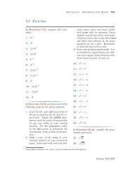
These commands change the spherical spiral to a dark shade of red and thicken<br />
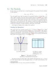
the spiral to 2pts. The result is shown <strong>in</strong> Figure 3.3. Because we changed the<br />
Alpha sett<strong>in</strong>gs (transparency) of the edges and faces of the sphere, note that we<br />
can “see through” the sphere to a certa<strong>in</strong> extent, mak<strong>in</strong>g the spherical spiral on<br />
the far side of the sphere visible.<br />
Viviani’s Curve<br />
Many new curves can be fromed from the <strong>in</strong>tersection of two surfaces. For example,<br />
all of the conic sections (circle, ellipse, parabola, and hyperbola) are determ<strong>in</strong>ed<br />
by how a plane <strong>in</strong>tersects a right-circular cone (we will explore these conic<br />
sections <strong>in</strong> the exercises).
Section <strong>3.5</strong> <strong>Space</strong> <strong>Curves</strong> <strong>in</strong> <strong>Matlab</strong> 245<br />
Figure 3.3. Superimpos<strong>in</strong>g the spherical spiral on a transparent<br />
sphere.<br />
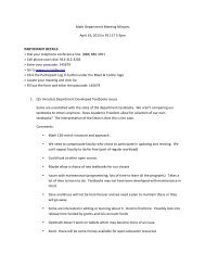
Such is the case with a space curve known as Viviani’s Curve, which is the<br />
<strong>in</strong>tersection of a sphere of radius 2r (centered at the orig<strong>in</strong>) and a right-circular<br />
cyl<strong>in</strong>der of radius r that is shifted r units along either the x- or y-axis.<br />
The equation of the sphere is x 2 + y 2 + z 2 = 4r 2 . We know that this sphere<br />
can be produced by the parametric equations<br />
x = 2r s<strong>in</strong> φ cos θ<br />
y = 2r s<strong>in</strong> φ s<strong>in</strong> θ<br />
z = 2r cos φ.<br />
(3.4)<br />
We offer the follow<strong>in</strong>g construction with few comments. It is similar to what we<br />
did <strong>in</strong> Example 2.<br />
r=1;<br />
phi=l<strong>in</strong>space(0,pi,30);<br />
theta=l<strong>in</strong>space(0,2*pi,40);<br />
[phi,theta]=meshgrid(phi,theta);<br />
x=2*r*s<strong>in</strong>(phi).*cos(theta);<br />
y=2*r*s<strong>in</strong>(phi).*s<strong>in</strong>(theta);<br />
z=2*r*cos(phi);<br />
Handle graphics are employed to color edges.
246 Chapter 3 Plott<strong>in</strong>g <strong>in</strong> <strong>Matlab</strong><br />
mhndl1=mesh(x,y,z)<br />
set(mhndl1,...<br />
’EdgeColor’,[0.6,0.6,0.6])<br />
axis equal<br />
axis off<br />
A circle of radius r centered at the orig<strong>in</strong> has equation x 2 + y 2 = r 2 . If we plot<br />
the set of all (x, y, z) such that x 2 + y 2 = r 2 , the result is a right-circular cyl<strong>in</strong>der<br />
of radius r. Replace x with x − r to get (x − r) 2 + y 2 = r 2 , which will shift<br />
the cyl<strong>in</strong>der r units <strong>in</strong> the x-direction. One f<strong>in</strong>al question rema<strong>in</strong>s. How can we<br />
parametrize the cyl<strong>in</strong>der (x − r) 2 + y 2 = r 2 ?<br />
It’s fairly straightforward to show that the parametric equations<br />
x = r cos t<br />
y = r s<strong>in</strong> t<br />
(<strong>3.5</strong>)<br />
produce a circle of radius r centered at the orig<strong>in</strong> 3 . This can be verified with<br />
<strong>Matlab</strong>’s comet or plot command 4 . To shift this r units <strong>in</strong> the x-direction add<br />
r to the equation for x to obta<strong>in</strong><br />
x = r + r cos t<br />
y = r s<strong>in</strong> t.<br />
Thus, the parametric equations of the right-circular cyl<strong>in</strong>der (x − r) 2 + y 2 = r 2<br />
are<br />
x = r + r cos t<br />
y = r s<strong>in</strong> t<br />
z = z.<br />
The key to plott<strong>in</strong>g the cyl<strong>in</strong>der <strong>in</strong> <strong>Matlab</strong> is to realize that x, y, and z are<br />
functions of both t and z. That is,<br />
x(t, z) = r + r cos t<br />
y(t, z) = r s<strong>in</strong> t<br />
z(t, z) = z.<br />
Therefore, the first task is to create a grid of (t, z) pairs.<br />
(3.6)<br />
It will suffice to let 0 ≤ t ≤ 2π. That should trace out the circle. If we hope<br />
to see the <strong>in</strong>tersection of the sphere (radius 2r) and the cyl<strong>in</strong>der, we will need to<br />
x2 + y2 = r2 cos2 t + r2 s<strong>in</strong> 2 t = r2 (cos2 t + s<strong>in</strong> 2 t) = r2 3<br />
.<br />
4<br />
And axis equal.
Section <strong>3.5</strong> <strong>Space</strong> <strong>Curves</strong> <strong>in</strong> <strong>Matlab</strong> 247<br />
have the cyl<strong>in</strong>der at least as low and high <strong>in</strong> the z-directions as is the sphere of<br />
radius 2r. Thus, limit −2r ≤ z ≤ 2r. After creat<strong>in</strong>g these vectors, we then create<br />
a grid of (t, z) pairs.<br />
t=l<strong>in</strong>space(0,2*pi,40);<br />
z=l<strong>in</strong>space(-2*r,2*r,20);<br />
[t,z]=meshgrid(t,z);<br />
Use the parametric equations (3.6) to produce po<strong>in</strong>ts (x, y, z) on the cyl<strong>in</strong>der<br />
as a function of the grid pairs (t, z).<br />
x=r+r*cos(t);<br />
y=r*s<strong>in</strong>(t);<br />
z=z;<br />
Hold the graph and plot the cyl<strong>in</strong>der. Handle graphics are used to color the edges.<br />
A view is set that allows the visualization of the <strong>in</strong>tersection of the sphere and<br />
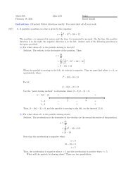
cyl<strong>in</strong>der. The result<strong>in</strong>g image is shown <strong>in</strong> Figure 3.4.<br />
hold on<br />
mhndl2=mesh(x,y,z)<br />
set(mhndl2,...<br />
’EdgeColor’,[0.8,0,0])<br />
view(50,20)<br />
Now, how do we get the parametrization of the curve of <strong>in</strong>tersection? Recall<br />
the equations of the sphere and cyl<strong>in</strong>der.<br />
x 2 + y 2 + z 2 = 4r 2<br />
(x − r) 2 + y 2 = r 2<br />
If we expand and simplify the second equation, we get<br />
x 2 − 2rx + y 2 = 0.<br />
If we subtract this result from the first equation, we obta<strong>in</strong><br />
z 2 + 2rx = 4r 2 .
248 Chapter 3 Plott<strong>in</strong>g <strong>in</strong> <strong>Matlab</strong><br />
Figure 3.4. The <strong>in</strong>tersection of the sphere and cyl<strong>in</strong>der is<br />
called Viviani’s Curve.<br />
Note that all po<strong>in</strong>ts on Viviani’s curve must fall on the cyl<strong>in</strong>der, where x =<br />
r + r cos t. Substitute this <strong>in</strong>to the last result.<br />
This can be written<br />
z 2 + 2r(r + r cos t) = 4r 2<br />
z 2 + 2r 2 + 2r 2 cos t = 4r 2<br />
z 2 = 4r 2<br />
z 2 = 2r 2 − 2r 2 cos t.<br />
1 − cos t<br />
2<br />
<br />
,<br />
and the half angle identity s<strong>in</strong> 2 (t/2) = (1 − cos t)/2 leads to<br />
z 2 = 4r 2 s<strong>in</strong> 2 (t/2).<br />
Normally, we should now say z = ±2r s<strong>in</strong>(t/2), but we will go with z = 2r s<strong>in</strong>(t/2)<br />
<strong>in</strong> the follow<strong>in</strong>g set of parametric equations for Viviani’s Curve.<br />
x = r + r cos t<br />
y = r s<strong>in</strong> t<br />
z = 2r s<strong>in</strong>(t/2).<br />
(3.7)<br />
Note that the period of z = 2r s<strong>in</strong>(t/2) is T = 4π, so if we go with only 0 ≤ t ≤ 2π,<br />
we will only get positive values of z and the lower half of the curve will not be<br />
shown 5 . Thus, we use 0 ≤ t ≤ 4π.
t=l<strong>in</strong>space(0,4*pi,200);<br />
Section <strong>3.5</strong> <strong>Space</strong> <strong>Curves</strong> <strong>in</strong> <strong>Matlab</strong> 249<br />
Use the parametric equation (3.7) to compute po<strong>in</strong>ts (x, y, z) on Viviani’s Curve<br />
<strong>in</strong> terms of t.<br />
x=r+r*cos(t);<br />
y=r*s<strong>in</strong>(t);<br />
z=2*r*s<strong>in</strong>(t/2);<br />
We plot the curve and record its “handle.” We then use handle graphics to color<br />
the curve black ([0, 0, 0] is black) and set the l<strong>in</strong>e width at 2 po<strong>in</strong>ts.<br />
vhndl=l<strong>in</strong>e(x,y,z)<br />
set(vhndl,...<br />
’Color’,[0,0,0],...<br />
’L<strong>in</strong>eWidth’,2)<br />
view(50,20)<br />
Sett<strong>in</strong>g the same view used <strong>in</strong> Figure 3.4 produces the image <strong>in</strong> Figure <strong>3.5</strong>.<br />
Figure <strong>3.5</strong>. The <strong>in</strong>tersection of the cyl<strong>in</strong>der and sphere is<br />
the curve of Viviani.<br />
5<br />
The reader should verify this statement is true.
250 Chapter 3 Plott<strong>in</strong>g <strong>in</strong> <strong>Matlab</strong><br />
You’ll want to click the rotate icon on the toolbar and use the mouse to rotate<br />
and twist the figure to verify that our parametrization of Viviani’s Curve is truly<br />
the <strong>in</strong>tersection of the sphere and cyl<strong>in</strong>der.
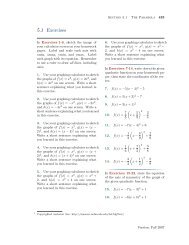
<strong>3.5</strong> Exercises<br />
In Exercises 1-6, perform each of the<br />
follow<strong>in</strong>g tasks.<br />
i. Sketch the space curve def<strong>in</strong>ed by<br />
the given set of parametric equations<br />
over the <strong>in</strong>dicated doma<strong>in</strong>.<br />
ii. Turn the box on, label each axis,<br />
and provide a title.<br />
1. On 0 ≤ t ≤ 1, sketch the Lissajous<br />
Curve<br />
x = 3 s<strong>in</strong>(4πt)<br />
y = 4 s<strong>in</strong>(6πt)<br />
z = 5 s<strong>in</strong>(8πt).<br />
2. On 0 ≤ t ≤ 1, sketch the Lissajous<br />
Curve<br />
x = 3 s<strong>in</strong>(4πt)<br />
y = 4 s<strong>in</strong>(10πt)<br />
z = 5 s<strong>in</strong>(14πt).<br />
3. On 0 ≤ t ≤ 2π, sketch the Torus<br />
Knot<br />
x = (6.25 + 3 cos 5t) cos 2t<br />
y = (6.25 + 3 cos 5t) s<strong>in</strong> 2t<br />
z = 3.25 s<strong>in</strong> 5t.<br />
4. On 0 ≤ t ≤ 2π, sketch the Torus<br />
Knot<br />
x = (7 + 2 cos 5t) cos 3t<br />
y = (7 + 2 cos 5t) s<strong>in</strong> 3t<br />
z = 3 s<strong>in</strong> 5t.<br />
5. On 0 ≤ t ≤ 6π, sketch the Trefoil<br />
Knot<br />
Section <strong>3.5</strong> <strong>Space</strong> <strong>Curves</strong> <strong>in</strong> <strong>Matlab</strong> 251<br />
x = cos t(2 − cos(2t/3))<br />
y = s<strong>in</strong> t(2 − cos(2t/3))<br />
z = − s<strong>in</strong>(2t/3).<br />
6. On 0 ≤ t ≤ 10π, sketch the C<strong>in</strong>quefoil<br />
Knot<br />
x = cos t(2 − cos(2t/5))<br />
y = s<strong>in</strong> t(2 − cos(2t/5))<br />
z = − s<strong>in</strong>(2t/5).<br />
In Exercises 7-10, we <strong>in</strong>vestigate the<br />
conic sections, each of which is the <strong>in</strong>tersection<br />
of a plane with a right circular<br />
cone. In each exercise, perform<br />
the follow<strong>in</strong>g tasks.<br />
i. Draw the right circular cone hav<strong>in</strong>g<br />
the parametric equations<br />
x = r cos θ<br />
y = r s<strong>in</strong> θ<br />
z = r,<br />
(3.8)<br />
where 0 ≤ θ ≤ 2π and −1 ≤ r ≤<br />
1. Use handle graphics to set the<br />
EdgeColor to a shade of gray.<br />
ii. Execute hold on to “hold” the surface<br />
plot of the right circular cone.<br />
Superimpose the plot of the given<br />
plane over the given doma<strong>in</strong>, then<br />
use <strong>Matlab</strong>’s handle graphics to set<br />
the EdgeColor to a s<strong>in</strong>gle color of<br />
your choice.<br />
iii. Click the rotate icon on the figure<br />
toolbar and rotate the figure to<br />
a view that emphasizes the conic<br />
section (curve of <strong>in</strong>tersection) and<br />
note the azimuth and elevation. Use
252 Chapter 3 Plott<strong>in</strong>g <strong>in</strong> <strong>Matlab</strong><br />
these components <strong>in</strong> the view(ax,el)<br />
<strong>in</strong> your script to obta<strong>in</strong> an identical<br />
view. Label the axes and provide<br />
a title that <strong>in</strong>cludes the name<br />
the conic section that is the <strong>in</strong>tersection<br />
of the given plane and the<br />
right circular cone.<br />
7. Sketch the plane z = 1/2 over the<br />
doma<strong>in</strong><br />
D = {(x, y) : −1 ≤ x, y ≤ 1}.<br />
8. Sketch the plane z = 0.4y + 0.5<br />
over the doma<strong>in</strong><br />
D = {(x, y) : −1 ≤ x, y ≤ 1}.<br />
9. Sketch the plane z = y+0.25 over<br />
the doma<strong>in</strong><br />
D = {(x, y) : −1 ≤ x, y ≤ 1}.<br />
10. Sketch the plane x = 0.5 over<br />
the doma<strong>in</strong><br />
D = {(y, z) : −1 ≤ y, z ≤ 1}.<br />
11. Sketch the torus def<strong>in</strong>ed by the<br />
parametric equations<br />
x = (7 + 2 cos u) cos v<br />
y = (7 + 2 cos u) s<strong>in</strong> v<br />
z = 3 s<strong>in</strong> u.<br />
Set the EdgeColor to a shade of gray<br />
and add transparency by sett<strong>in</strong>g both<br />
FaceAlpha and EdgeAlpha equal<br />
to 0.5. Set the axis equal. Use <strong>Matlab</strong>’s<br />
l<strong>in</strong>e command to superimpose<br />
the torus knot hav<strong>in</strong>g parmetric equations<br />
x = (7 + 2 cos 5t) cos 2t<br />
y = (7 + 2 cos 5t) s<strong>in</strong> 2t<br />
z = 3 s<strong>in</strong> 5t<br />
over the time doma<strong>in</strong> 0 ≤ t ≤ 2π.<br />
Use handle graphics to set the Color<br />
of the torus knot to a color of your<br />
choice and set the L<strong>in</strong>eWidth to a<br />
thickness of 2 po<strong>in</strong>ts.<br />
12. Sketch the torus def<strong>in</strong>ed by the<br />
parametric equations<br />
x = (8 + 2 cos u) cos v<br />
y = (8 + 2 cos u) s<strong>in</strong> v<br />
z = 3 s<strong>in</strong> u.<br />
Set the EdgeColor to a shade of gray<br />
and add transparency by sett<strong>in</strong>g both<br />
FaceAlpha and EdgeAlpha equal<br />
to 0.5. Set the axis equal. Use <strong>Matlab</strong>’s<br />
l<strong>in</strong>e command to superimpose<br />
the torus knot hav<strong>in</strong>g parmetric equations<br />
x = (8 + 2 cos 11t) cos 3t<br />
y = (8 + 2 cos 11t) s<strong>in</strong> 3t<br />
z = 3 s<strong>in</strong> 11t<br />
over the time doma<strong>in</strong> 0 ≤ t ≤ 2π.<br />
Use handle graphics to set the Color<br />
of the torus knot to a color of your<br />
choice and set the L<strong>in</strong>eWidth to a<br />
thickness of 2 po<strong>in</strong>ts.<br />
13. Sketch the cone def<strong>in</strong>ed by the<br />
parametric equations<br />
x = r cos θ<br />
y = r s<strong>in</strong> θ<br />
z = r<br />
where 0 ≤ r ≤ 1 and 0 ≤ θ ≤ 2π.<br />
Set the EdgeColor to a shade of gray
and add transparency by sett<strong>in</strong>g both<br />
FaceAlpha and EdgeAlpha equal<br />
to 0.5. Set the axis equal. Use <strong>Matlab</strong>’s<br />
l<strong>in</strong>e command to superimpose<br />
the conical spiral hav<strong>in</strong>g parmetric equations<br />
x = t cos 20t<br />
y = t s<strong>in</strong> 20t<br />
z = t<br />
over the time doma<strong>in</strong> 0 ≤ t ≤ 1. Use<br />
handle graphics to set the Color of<br />
the conical spiral to a color of your<br />
choice and set the L<strong>in</strong>eWidth to a<br />
thickness of 2 po<strong>in</strong>ts.<br />
14. Sketch the cyl<strong>in</strong>der def<strong>in</strong>ed by<br />
the parametric equations<br />
x = 2 cos θ<br />
y = 2 s<strong>in</strong> θ<br />
z = z,<br />
where 0 ≤ z ≤ 5 and 0 ≤ θ ≤ 2π.<br />
Set the EdgeColor to a shade of gray<br />
and add transparency by sett<strong>in</strong>g both<br />
FaceAlpha and EdgeAlpha equal<br />
to 0.5. Set the axis equal. Use <strong>Matlab</strong>’s<br />
l<strong>in</strong>e command to superimpose<br />
the helix hav<strong>in</strong>g parmetric equations<br />
x = 2 cos 5t<br />
y = 2 s<strong>in</strong> 5t<br />
z = t,<br />
over the time doma<strong>in</strong> 0 ≤ t ≤ 5. Use<br />
handle graphics to set the Color of<br />
the helix to a color of your choice and<br />
set the L<strong>in</strong>eWidth to a thickness of<br />
2 po<strong>in</strong>ts.<br />
15. Challenge. The <strong>in</strong>tersection of<br />
a sphere and a plane that passes through<br />
Section <strong>3.5</strong> <strong>Space</strong> <strong>Curves</strong> <strong>in</strong> <strong>Matlab</strong> 253<br />
the center of the sphere is called a<br />
great circle. Sketch the equation of<br />
a sphere of radius 1, then sketch the<br />
plane y = x and show that the <strong>in</strong>tersection<br />
is a great circle. F<strong>in</strong>d the<br />
parametric equations of this great circle<br />
and add it to your plot.
254 Chapter 3 Plott<strong>in</strong>g <strong>in</strong> <strong>Matlab</strong><br />
<strong>3.5</strong> Answers<br />
1.<br />
3.<br />
t=l<strong>in</strong>space(0,1,200);<br />
x=3*s<strong>in</strong>(4*pi*t);<br />
y=4*s<strong>in</strong>(6*pi*t);<br />
z=5*s<strong>in</strong>(8*pi*t);<br />
plot3(x,y,z)<br />
box on<br />
view(135,30)<br />
t=l<strong>in</strong>space(0,2*pi,200);<br />
x=(6.25+3*cos(5*t)).*cos(2*t);<br />
y=(6.25+3\cos(5*t)).*s<strong>in</strong>(2*t);<br />
z=3.25*s<strong>in</strong>(5*t);<br />
plot3(x,y,z)<br />
box on<br />
view(135,30)<br />
5.<br />
t=l<strong>in</strong>space(0,6*pi,200);<br />
x=cos(t).*(2-cos(2*t/3));<br />
y=s<strong>in</strong>(t).*(2-cos(2*t/3));<br />
z=-s<strong>in</strong>(2*t/3);<br />
plot3(x,y,z)<br />
box on<br />
view(135,30)
7. Set the grid for the cone.<br />
theta=l<strong>in</strong>space(0,2*pi,40);<br />
r=l<strong>in</strong>space(-1,1,30);<br />
[theta,r]=meshgrid(theta,r);<br />
Use the parametric equations to<br />
compute x, y, and z.<br />
x=r.*cos(theta);<br />
y=r.*s<strong>in</strong>(theta);<br />
z=r;<br />
Draw the right circular cone <strong>in</strong> a<br />
shade of gray.<br />
mhndl=mesh(x,y,z)<br />
set(mhndl,...<br />
’EdgeColor’,[.6,.6,.6])<br />
Hold the surface plot and draw<br />
the plane z = 1/2.<br />
Section <strong>3.5</strong> <strong>Space</strong> <strong>Curves</strong> <strong>in</strong> <strong>Matlab</strong> 255<br />
hold on<br />
[x,y]=meshgrid(-1:0.2:1);<br />
z=0.5*ones(size(x));<br />
phndl=mesh(x,y,z);<br />
set(phndl,...<br />
’EdgeColor’,[0.625,0,0])<br />
Adjust orientation.<br />
axis equal<br />
view(116,38)<br />
Annotate the plot <strong>in</strong> the usual manner.<br />
The <strong>in</strong>tersection is a circle, as<br />
<strong>in</strong>dicated <strong>in</strong> the title.<br />
9. Set the grid for the cone.<br />
theta=l<strong>in</strong>space(0,2*pi,40);<br />
r=l<strong>in</strong>space(-1,1,30);<br />
[theta,r]=meshgrid(theta,r);<br />
Use the parametric equations to
256 Chapter 3 Plott<strong>in</strong>g <strong>in</strong> <strong>Matlab</strong><br />
compute x, y, and z.<br />
x=r.*cos(theta);<br />
y=r.*s<strong>in</strong>(theta);<br />
z=r;<br />
Draw the right circular cone <strong>in</strong> a<br />
shade of gray.<br />
mhndl=mesh(x,y,z)<br />
set(mhndl,...<br />
’EdgeColor’,[.6,.6,.6])<br />
Hold the surface plot and draw<br />
the plane z = y + 0.25.<br />
hold on<br />
[[x,y]=meshgrid(-1:0.1:1);<br />
z=y+0.25;<br />
phndl=mesh(x,y,z);<br />
set(phndl,...<br />
’EdgeColor’,[0.625,0,0])<br />
Adjust orientation.<br />
axis equal<br />
view(77,50)<br />
Annotate the plot <strong>in</strong> the usual manner.<br />
The <strong>in</strong>tersection is a parabola, as<br />
<strong>in</strong>dicated <strong>in</strong> the title.<br />
11. Set parameters a, b, and c.<br />
a=7;b=2;c=3;<br />
Set the grid for the torus.<br />
u=l<strong>in</strong>space(0,2*pi,20);<br />
v=l<strong>in</strong>space(0,2*pi,40);<br />
[u,v]=meshgrid(u,v);<br />
Use the parametric equations to<br />
compute x, y, and z.<br />
x=(a+b*cos(u)).*cos(v);<br />
y=(a+b*cos(u)).*s<strong>in</strong>(v);<br />
z=c*s<strong>in</strong>(u);<br />
Draw the torus <strong>in</strong> a shade of gray<br />
and add transparency. Set the perspective<br />
with axis equal.
mhndl=mesh(x,y,z);<br />
set(mhndl,...<br />
’EdgeColor’,[.6,.6,.6],...<br />
’FaceAlpha’,0.5,...<br />
’EdgeAlpha’,0.5);<br />
axis equal<br />
Compute x, y, and z for the torus<br />
knot over the requested time doma<strong>in</strong>.<br />
t=l<strong>in</strong>space(0,2*pi,200);<br />
x=(a+b*cos(5*t)).*cos(2*t);<br />
y=(a+b*cos(5*t)).*s<strong>in</strong>(2*t);<br />
z=c*s<strong>in</strong>(5*t);<br />
Plot the torus knot and change<br />
its color and l<strong>in</strong>ewidth.<br />
lhndl=l<strong>in</strong>e(x,y,z);<br />
set(lhndl,...<br />
’Color’,[.625,0,0],...<br />
’L<strong>in</strong>eWidth’,2)<br />
Adjust orientation.<br />
view(135,30)<br />
Annotate the plot <strong>in</strong> the usual<br />
manner.<br />
Section <strong>3.5</strong> <strong>Space</strong> <strong>Curves</strong> <strong>in</strong> <strong>Matlab</strong> 257<br />
13. Set the grid for the cone.<br />
r=l<strong>in</strong>space(0,1,20);<br />
theta=l<strong>in</strong>space(0,2*pi,40);<br />
[r,theta]=meshgrid(r,theta);<br />
Use the parametric equations to<br />
compute x, y, and z.<br />
x=r.*cos(theta);<br />
y=r.*s<strong>in</strong>(theta);<br />
z=r;<br />
Draw the cone <strong>in</strong> a shade of gray<br />
and add transparency. Set the perspective<br />
with axis equal.<br />
mhndl=mesh(x,y,z);<br />
set(mhndl,...<br />
’EdgeColor’,[.6,.6,.6],...<br />
’FaceAlpha’,0.5,...<br />
’EdgeAlpha’,0.5);<br />
axis equal
258 Chapter 3 Plott<strong>in</strong>g <strong>in</strong> <strong>Matlab</strong><br />
Compute x, y, and z for the conical<br />
spiral over the requested time doma<strong>in</strong>.<br />
t=l<strong>in</strong>space(0,1,200);<br />
x=t.*cos(20*t);<br />
y=t.*s<strong>in</strong>(20*t);<br />
z=t;<br />
Plot the concical spiral and change<br />
its color and l<strong>in</strong>ewidth.<br />
lhndl=l<strong>in</strong>e(x,y,z);<br />
set(lhndl,...<br />
’Color’,[.625,0,0],...<br />
’L<strong>in</strong>eWidth’,2)<br />
Adjust orientation.<br />
view(135,30)<br />
Annotate the plot <strong>in</strong> the usual<br />
manner.