3.5 Space Curves in Matlab

More documents

Recommendations

Info

$Math 50A February 18, 2011 Quiz #10 Name: David Arnold ...$

$College of the Redwoods Math Lab What is the Math Lab course? The$

$Math Department Meeting Minutes April 19, 2013 in PS 117 3-â€5pm ...$

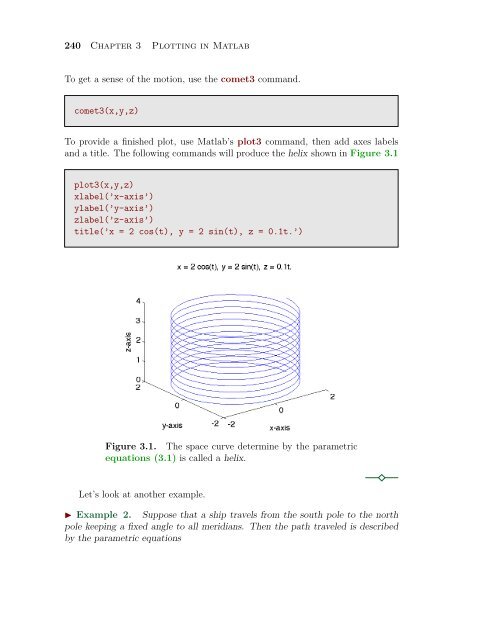
240 Chapter 3 Plotting in Matlab To get a sense of the motion, use the comet3 command. comet3(x,y,z) To provide a finished plot, use Matlab’s plot3 command, then add axes labels and a title. The following commands will produce the helix shown in Figure 3.1 plot3(x,y,z) xlabel(’x-axis’) ylabel(’y-axis’) zlabel(’z-axis’) title(’x = 2 cos(t), y = 2 sin(t), z = 0.1t.’) Figure 3.1. The space curve determine by the parametric equations (3.1) is called a helix. Let’s look at another example. ◮ Example 2. Suppose that a ship travels from the south pole to the north pole keeping a fixed angle to all meridians. Then the path traveled is described by the parametric equations
Section 3.5 Space Curves in Matlab 241 x = y = z = − cos t √ 1 + α 2 t 2 sin t √ 1 + α 2 t 2 Set α = 0.2 and restrict −12π ≤ t ≤ 12π. αt √ 1 + α 2 t 2 . (3.2) Set α = 0.2 and create a vector of t-values subject to the constraint −12π ≤ t ≤ 12π. alpha=0.2; t=linspace(-12*pi,12*pi,500); Use the parametric equations (3.2) to compute the positions (x, y, z) on the spherical spiral as a function of time t. x=cos(t)./sqrt(1+alpha^2*t.^2); y=sin(t)./sqrt(1+alpha^2*t.^2); z=alpha*t./sqrt(1+alpha^2*t.^2); Use comet3 to animate the motion, then follow this with Matlab’s plot3 command. This will produce the spherical spiral shown in Figure 3.2. plot3(x,y,z) Handle Graphics Many space curves are closely related with one or another particular class of surfaces. In the case of the spherical spiral, one would intuit a close relationship with a sphere. So, let’s draw a sphere of appropriate radius, then superimpose the spherical spiral of Example 2. In the section on Parametric Surfaces, we saw the parametric equations of a sphere of radius r, which we repeat here for convenience.
Page 1: 3.5 Space Curves in Matlab Section
Page 5 and 6: mhndl=mesh(x,y,z) Section 3.5 Space
Page 7 and 8: Section 3.5 Space Curves in Matlab
Page 9 and 10: Section 3.5 Space Curves in Matlab
Page 11 and 12: t=linspace(0,4*pi,200); Section 3.5
Page 13 and 14: 3.5 Exercises In Exercises 1-6, per
Page 15 and 16: and add transparency by setting bot
Page 17 and 18: 7. Set the grid for the cone. theta
Page 19 and 20: mhndl=mesh(x,y,z); set(mhndl,...

3.5 Space Curves in Matlab

Create successful ePaper yourself

Delete template?

Save as template?