3.5 Space Curves in Matlab
3.5 Space Curves in Matlab
3.5 Space Curves in Matlab

You also want an ePaper? Increase the reach of your titles
YUMPU automatically turns print PDFs into web optimized ePapers that Google loves.
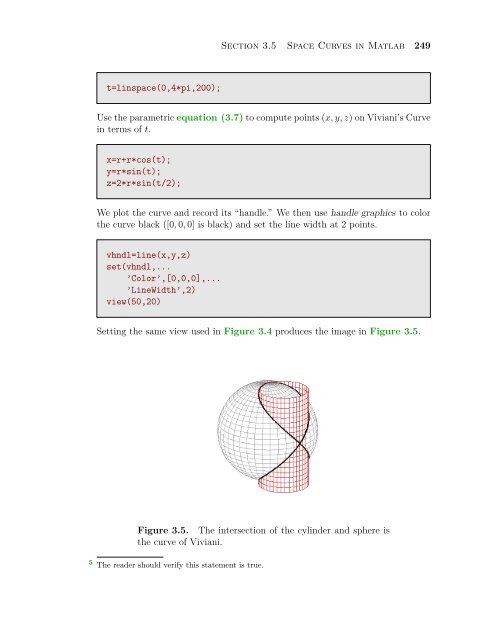
t=l<strong>in</strong>space(0,4*pi,200);<br />
Section <strong>3.5</strong> <strong>Space</strong> <strong>Curves</strong> <strong>in</strong> <strong>Matlab</strong> 249<br />
Use the parametric equation (3.7) to compute po<strong>in</strong>ts (x, y, z) on Viviani’s Curve<br />
<strong>in</strong> terms of t.<br />
x=r+r*cos(t);<br />
y=r*s<strong>in</strong>(t);<br />
z=2*r*s<strong>in</strong>(t/2);<br />
We plot the curve and record its “handle.” We then use handle graphics to color<br />
the curve black ([0, 0, 0] is black) and set the l<strong>in</strong>e width at 2 po<strong>in</strong>ts.<br />
vhndl=l<strong>in</strong>e(x,y,z)<br />
set(vhndl,...<br />
’Color’,[0,0,0],...<br />
’L<strong>in</strong>eWidth’,2)<br />
view(50,20)<br />
Sett<strong>in</strong>g the same view used <strong>in</strong> Figure 3.4 produces the image <strong>in</strong> Figure <strong>3.5</strong>.<br />
Figure <strong>3.5</strong>. The <strong>in</strong>tersection of the cyl<strong>in</strong>der and sphere is<br />
the curve of Viviani.<br />
5<br />
The reader should verify this statement is true.