3.5 Space Curves in Matlab
3.5 Space Curves in Matlab
3.5 Space Curves in Matlab

You also want an ePaper? Increase the reach of your titles
YUMPU automatically turns print PDFs into web optimized ePapers that Google loves.
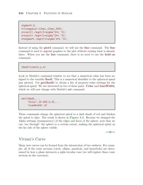
244 Chapter 3 Plott<strong>in</strong>g <strong>in</strong> <strong>Matlab</strong><br />
alpha=0.2;<br />
t=l<strong>in</strong>space(-12*pi,12*pi,500);<br />
x=cos(t)./sqrt(1+alpha^2*t.^2);<br />
y=s<strong>in</strong>(t)./sqrt(1+alpha^2*t.^2);<br />
z=alpha*t./sqrt(1+alpha^2*t.^2);<br />
Instead of us<strong>in</strong>g the plot3 command, we will use the l<strong>in</strong>e command. The l<strong>in</strong>e<br />
command is used to append graphics to the plot without eras<strong>in</strong>g what is already<br />
there. When you use the l<strong>in</strong>e command, there is no need to use the hold on<br />
command.<br />
lhndl=l<strong>in</strong>e(x,y,z)<br />
Look <strong>in</strong> <strong>Matlab</strong>’s command w<strong>in</strong>dow to see that a numerical value has been assigned<br />
to the variable lhndl. This is a numerical identifier to the spherical spiral<br />
just plotted. Use get(lhndl) to obta<strong>in</strong> a list of property-value sett<strong>in</strong>gs for the<br />
spherical spiral. We are <strong>in</strong>terested <strong>in</strong> two of these pairs: Color and L<strong>in</strong>eWidth,<br />
which we will now change with <strong>Matlab</strong>’s set command.<br />
set(lhndl,...<br />
’Color’,[0.625,0,0],...<br />
’L<strong>in</strong>eWidth’,2)<br />
These commands change the spherical spiral to a dark shade of red and thicken<br />
the spiral to 2pts. The result is shown <strong>in</strong> Figure 3.3. Because we changed the<br />
Alpha sett<strong>in</strong>gs (transparency) of the edges and faces of the sphere, note that we<br />
can “see through” the sphere to a certa<strong>in</strong> extent, mak<strong>in</strong>g the spherical spiral on<br />
the far side of the sphere visible.<br />
Viviani’s Curve<br />
Many new curves can be fromed from the <strong>in</strong>tersection of two surfaces. For example,<br />
all of the conic sections (circle, ellipse, parabola, and hyperbola) are determ<strong>in</strong>ed<br />
by how a plane <strong>in</strong>tersects a right-circular cone (we will explore these conic<br />
sections <strong>in</strong> the exercises).