K. Kobayashi and S. Tsumura

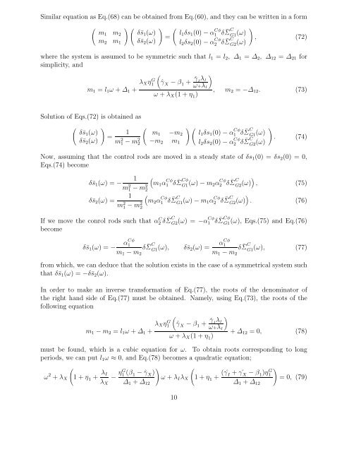
Similar equation as Eq.(68) can be obtained from Eq.(60), and they can be written in a form
m1 m2
m2 m1
δ¯s1(ω)
δ¯s2(ω)
=
l1δs1(0) − α Cφ
1 δ ¯ Σ C
G1 (ω)
l2δs2(0) − α Cφ
2 δ ¯ Σ C
G2(ω)
, (72)
where the system is assumed to be symmetric such that l1 = l2, ∆1 = ∆2, ∆12 = ∆21 for
simplicity, and
m1 = l1ω + ∆1 +
Solution of Eqs.(72) is obtained as
δ¯s1(ω)
δ¯s2(ω)
=
1
m 2 1 − m 2 2
λXη G 1
ˆγ X − β 1 + ˆγ IλI
ω + λX(1 + η 1)
m1 −m2
−m2 m1
ω+λI
, m2 = −∆12. (73)
l1δs1(0) − α Cφ
1 δ ¯ Σ C
G1(ω)
l2δs2(0) − α Cφ
2 δ ¯ Σ C
G2 (ω)
. (74)
Now, assuming that the control rods are moved in a steady state of δs1(0) = δs2(0) = 0,
Eqs.(74) become
1
δ¯s1(ω) =−
m2 1 − m2
m1α
2
Cφ
1 δ ¯ Σ Cφ
Cφ
G1 (ω) − m2α2 δ ¯ Σ C
G2 (ω) , (75)
1
δ¯s2(ω) =
m2 1 − m2
m2α
2
Cφ
1 δ ¯ Σ C
G1(ω) − m1α Cφ
2 δ ¯ Σ C
G2(ω)
. (76)
If we move the conrol rods such that αC 2 δ ¯ Σ C
G2(ω) =−α Cφ
1 δ ¯ Σ Cφ
G1(ω), Eqs.(75) and Eq.(76)
become
δ¯s1(ω) =− αCφ 1
δ
m1 − m2
¯ Σ C
G1 (ω), δ¯s2(ω) = αCφ 1
m1 − m2
δ ¯ Σ C
G1 (ω), (77)
from which, we can deduce that the solution exists in the case of a symmetrical system such
that δ¯s1(ω) =−δ¯s2(ω).
In order to make an inverse transformation of Eq.(77), the roots of the denominator of
the right hand side of Eq.(77) must be obtained. Namely, using Eq.(73), the roots of the
following equation
m1 − m2 = l1ω + ∆1 +
λXη G 1
ˆγ X − β 1 + ˆγ IλI
ω + λX(1 + η 1)
ω+λI
+ ∆12 =0, (78)
must be found, which is a cubic equation for ω. To obtain roots corresponding to long
periods, we can put l1ω ≈ 0, and Eq.(78) becomes a quadratic equation;
ω 2 + λX
1+η 1 + λI
λX
− ηG
1 (β1 − ˆγ X)
ω + λIλX 1+η1 +
∆1 + ∆12
(ˆγ I + γˆX − β1)η G 1
∆1 + ∆12
10
=0, (79)