K. Kobayashi and S. Tsumura

of time. Substituting these iodine and xenon into the steady state equations (55), namely
I 0 m + δIm(t) = ˆγ I
s
λI
I m (t), X0 m + δXm(t) = (ˆγ I +ˆγ X)sX m(t)
λX +ˆσ 00
XmsXm (t).
(109)
fictitious production rates sI m (t) and sXm (t) corresponding to the iodine and xenon densities,
respectively, for non-steady state, are calculated. Using these fictitious production rates,
two axial offsets are defined by
AOI = sI1(t) − sI 2(t)
sI 1(t)+sI 2(t) = δsI1(t) − δsI 2(t)
s0 1 + s0 ,
2
AOX = sX1 (t) − sX 2 (t)
sX 1 (t)+sX 2 (t) = δsX 1 (t) − δsX 2 (t)
s0 1 + s0 .
2
(110)
When the xenon oscillation exists, δs I m (t) and δsX m (t) as well as δs1(t) and δs2(t) are not
equal to zero, and the three axial offsets AOP , AOI and AOX take in general different values.
When all these three axial offsets become zero, the xenon oscillation stops and the system
returns to the steady state. Making use of this fact, a trajectory is plotted as a function of
time in a figure where the horizontal axis is AOP − AOX and the vertical axis is AOI − AOX,
and control rods are moved such that the state point on the trajectory moves to the origin
of the coordinates. In the method by Shimazu, the kinetics equations for neutrons are not
used, and only two point kinetics equations for iodine and xenon of Eqs.(56) and (57) are
solved. One of the advantages of this method is that it is easy to understand the xenon
oscillation and its control visually on a figure. In the present work, the kinetics equations
for neutrons are solved and special future of the axial offsets trajectory method can be
understood mathematically.
3. APPLICATION TO A ONE GROUP PROBLEM IN SLAB GEOMETRY
In order to investigate the applicability of the two point kinetics equations derived in the
preceding section analytically, we consider a simple one group problem in slab geometry.
3..1 CALCULATION OF COUPLING COEFFICIENTS
Let us calculate the kinetics parameters, the coupling coefficients analytically. The system
is assumed to be a coupled reactor of two symmetrical cores shown in Fig.1 in order to
compare the result with the previous one6) . Equation (4) for the importance function to
produce fission neutrons becomes
−D d2
+ Σa Gm(x) =νΣfδm(x), (111)
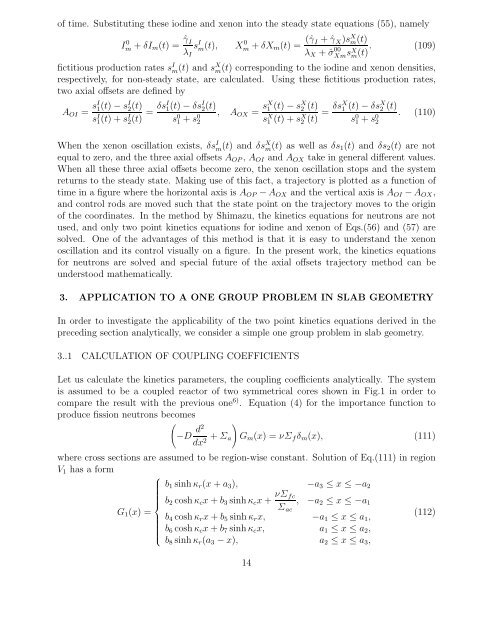
dx2 where cross sections are assumed to be region-wise constant. Solution of Eq.(111) in region
V1 has a form
⎧
b1 sinh κr(x + a3), −a3 ≤ x ≤−a2
⎪⎨ b2 cosh κcx + b3 sinh κcx +
G1(x) =
⎪⎩
νΣfc
, −a2 ≤ x ≤−a1
Σac
b4 cosh κrx + b5 sinh κrx, −a1 ≤ x ≤ a1,
b6 cosh κcx + b7 sinh κcx, a1 ≤ x ≤ a2,
b8 sinh κr(a3 − x), a2≤x≤a3, 14
(112)