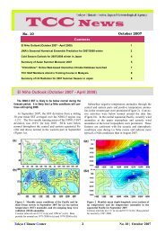
TCC News No. 30
TCC News No. 30
TCC News No. 30

Create successful ePaper yourself
Turn your PDF publications into a flip-book with our unique Google optimized e-Paper software.
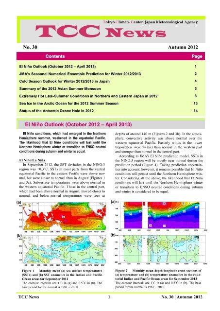
<strong>No</strong>. <strong>30</strong> Autumn 2012<br />
El Niño Outlook (October 2012 – April 2013)<br />
JMA’s Seasonal Numerical Ensemble Prediction for Winter 2012/2013<br />
Cold Season Outlook for Winter 2012/2013 in Japan<br />
Summary of the 2012 Asian Summer Monsoon<br />
Extremely Hot Late-Summer Conditions in <strong>No</strong>rthern and Eastern Japan in 2012<br />
Sea Ice in the Arctic Ocean for the 2012 Summer Season<br />
Status of the Antarctic Ozone Hole in 2012<br />
El Niño conditions, which had emerged in the <strong>No</strong>rthern<br />
Hemisphere summer, weakened in the equatorial Pacific.<br />
The likelihood that El Niño conditions will last until the<br />
<strong>No</strong>rthern Hemisphere winter or transition to ENSO neutral<br />
conditions during autumn and winter is equal.<br />
El Niño/La Niña<br />
In September 2012, the SST deviation in the NINO.3<br />
region was +0.3°C. SSTs in most parts from the central<br />
equatorial Pacific to the eastern Pacific were above normal,<br />
but were closer to normal than in August (Figures 1<br />
and 3a). Subsurface temperatures were above normal in<br />
the western equatorial Pacific. Those in the central part,<br />
which had been above normal in August, moved closer to<br />
normal, and below-normal temperatures were seen at<br />
(a)<br />
(b)<br />
Contents Page<br />
El Niño Outlook (October 2012 – April 2013)<br />
Figure 1 Monthly mean (a) sea surface temperatures<br />
(SSTs) and (b) SST anomalies in the Indian and Pacific<br />
Ocean areas for September 2012<br />
The contour intervals are 1˚C in (a) and 0.5˚C in (b). The<br />
base period for the normal is 1981 – 2010.<br />
<strong>TCC</strong> <strong>News</strong> 1 <strong>No</strong>. <strong>30</strong> | Autumn 2012<br />
(a)<br />
(b)<br />
depths of around 140 m (Figures 2 and 3b). In the atmosphere,<br />
convective activity was above normal over the<br />
western equatorial Pacific. Easterly winds in the lower<br />
troposphere were weaker than normal in the western part<br />
and stronger than normal in the central part.<br />
According to JMA's El Niño prediction model, SSTs in<br />
the NINO.3 region will be mostly near normal during the<br />
prediction period (Figure 4). Taking prediction uncertainties<br />
into account, however, it remains possible that El Niño<br />
conditions will persist until the <strong>No</strong>rthern Hemisphere winter.<br />
Considering all the above, the likelihood that El Niño<br />
conditions will last until the <strong>No</strong>rthern Hemisphere winter<br />
or transition to ENSO neutral conditions during autumn<br />
and winter is considered to be equal.<br />
Figure 2 Monthly mean depth-longitude cross sections of<br />
(a) temperature and (b) temperature anomalies in the equatorial<br />
Indian and Pacific Ocean areas for September 2012<br />
The contour intervals are 1˚C in (a) and 0.5˚C in (b). The base<br />
period for the normal is 1981 – 2010.<br />
1<br />
2<br />
4<br />
5<br />
8<br />
13<br />
14
(a) (b)<br />
Figure 3 Time-longitude cross sections of (a) SST and (b) ocean heat content (OHC) anomalies along the equator<br />
in the Indian and Pacific Ocean areas<br />
OHCs are defined here as vertical averaged temperatures in the top <strong>30</strong>0 m. The base period for the normal is 1981 – 2010.<br />
Western Pacific and Indian Ocean<br />
The area-averaged SST in the tropical western Pacific<br />
(NINO.WEST) region was below normal in<br />
September, and is likely to be near normal or below<br />
normal in the months ahead.<br />
The area-averaged SST in the tropical Indian<br />
Ocean (IOBW) region was near normal in September,<br />
and is likely to be near normal in the months ahead.<br />
(Ichiro Ishikawa, Climate Prediction Division)<br />
* The SST normals for the NINO.WEST region (Eq.<br />
– 15°N, 1<strong>30</strong>°E – 150°E) and the IOBW region (20°S<br />
– 20°N, 40°E – 100°E) are defined as linear extrapolations<br />
with respect to a sliding <strong>30</strong>-year period in<br />
order to remove the effects of long-term trends.<br />
According to JMA’s seasonal ensemble prediction<br />
system, convection is expected to be active over the<br />
tropical Indian Ocean and the central equatorial Pacific<br />
and inactive around the Maritime Continent and east of<br />
the Philippines. In association with active convection<br />
over the tropical Indian Ocean, the sub-tropical jet stream<br />
is expected to shift northward over the western part of<br />
the Eurasian Continent and air temperatures are expected<br />
to be above normal around South Asia. Conversely, negative<br />
anomalies of air temperature are expected over the<br />
mid-latitudes of the Eurasian Continent.<br />
Figure 4 Outlook of NINO.3 SST deviation produced by<br />
the El Niño prediction model<br />
This figure shows a time series of monthly NINO.3 SST deviations.<br />
The thick line with closed circles shows observed SST<br />
deviations, and the boxes show the values produced for the next<br />
six months by the El Niño prediction model. Each box denotes<br />
the range into which the SST deviation is expected to fall with a<br />
probability of 70%.<br />
JMA’s Seasonal Numerical Ensemble Prediction for Winter 2012/2013<br />
1. Introduction<br />
This article outlines JMA’s dynamical seasonal ensemble<br />
prediction for winter 2012/2013 (December 2012 –<br />
February 2013, referred to as DJF), which was used as a<br />
basis for the Agency’s operational cold-season outlook<br />
issued on 25 October, 2012. The outlook shown here is<br />
based on the seasonal ensemble prediction system of the<br />
Coupled atmosphere-ocean General Circulation Model<br />
(CGCM). See the column below for details of the system.<br />
Section 2 outlines global SST anomaly predictions, and<br />
Section 3 describes the circulation fields expected over<br />
the tropics and sub-tropics in association with these<br />
anomalies. Finally, the circulation fields predicted for the<br />
mid- and high latitudes of the <strong>No</strong>rthern Hemisphere are<br />
discussed in Section 4.<br />
<strong>TCC</strong> <strong>News</strong> 2 <strong>No</strong>. <strong>30</strong> | Autumn 2012
2. SST anomalies (Figure 5)<br />
Figure 5 shows predicted SSTs and their anomalies for<br />
DJF. Above-normal values are expected in the central part<br />
of the equatorial Pacific and the tropical Indian Ocean.<br />
3. Prediction for the tropics and sub-tropics (Figure 6)<br />
Figure 6 (a) shows predicted precipitation and related<br />
anomalies for DJF. In association with the SST anomaly<br />
pattern over the equatorial Pacific, precipitation is expected<br />
to be above normal over the central equatorial Pacific<br />
and below normal around the Maritime Continent<br />
and east of the Philippines. From the tropical Indian<br />
Ocean to Southeast Asia, above-normal precipitation is<br />
expected. However, the results of hindcast experimentation<br />
indicate that the level of prediction skill for precipitation<br />
around Southeast Asia is relatively low. Accordingly,<br />
the prediction of above-normal levels over Southeast Asia<br />
and the related response to the large-scale atmospheric<br />
circulation detailed later should be interpreted with caution.<br />
Velocity potential in the upper troposphere (200 hPa)<br />
(Figure 6 (b)) is expected to be negative (i.e., more divergent)<br />
over the tropical Indian Ocean and the central equatorial<br />
Pacific, reflecting active convection in these regions.<br />
Around the maritime continent, relatively positive<br />
(i.e., more convergent) anomalies are predicted, reflecting<br />
inactive convection.<br />
The stream function at 200 hPa (Figure 6 (c)) is generally<br />
expected to be negative (i.e., cyclonic) in the<br />
mid-latitudes of the <strong>No</strong>rthern Hemisphere, reflecting the<br />
zonal pattern of precipitation (i.e., active near the equator<br />
and inactive in the subtropics of the <strong>No</strong>rthern Hemisphere).<br />
From South to Southeast Asia, positive (i.e., an-<br />
<strong>TCC</strong> <strong>News</strong> 3 <strong>No</strong>. <strong>30</strong> | Autumn 2012<br />
SST<br />
(a)Precipitation (a)Precipitation<br />
(c)PSI200 (c)PSI200<br />
(b)CHI200 (b)CHI200<br />
Figure 5 Predicted SSTs (contours) and SST anomalies<br />
(shading) for December 2012 – February 2013 (ensemble<br />
mean of 51 members)<br />
ti-cyclonic) anomalies are expected, reflecting active<br />
convection from the tropical Indian Ocean to Southeast<br />
Asia. In association with this, the sub-tropical jet stream is<br />
expected to shift northward over the western part of the<br />
Eurasian Continent and above-normal air temperatures are<br />
expected around South Asia (not shown). However, the<br />
prediction of these anomalies around Southeast Asia<br />
should be interpreted with caution because they may be<br />
affected by active convection over Southeast Asia, which<br />
is predicted with insufficient reliability.<br />
Stream function anomalies at 850 hPa (Figure 6 (d)) are<br />
expected to be negative over the northern Indian Ocean in<br />
association with active convection in the region. Positive<br />
anomalies are predicted over the western tropical Pacific<br />
in association with inactive convection around the Maritime<br />
Continent and east of the Philippines.<br />
(d)PSI850 (d)PSI850<br />
Figure 6 Predicted atmospheric fields from 60°N – 60°S for December 2012 – February 2013 (ensemble<br />
mean of 51 members)<br />
(a) Precipitation (contours) and anomaly (shading). The contour interval is 2 mm/day.<br />
(b) Velocity potential at 200 hPa (contours) and anomaly (shading). The contour interval is 2 × 10 6 m 2 /s.<br />
(c) Stream function at 200 hPa (contours) and anomaly (shading). The contour interval is 16 × 10 6 m 2 /s.<br />
(d) Stream function at 850 hPa (contours) and anomaly (shading). The contour interval is 5 × 10 6 m 2 /s.
4. Prediction for the mid- and high latitudes of the<br />
<strong>No</strong>rthern Hemisphere (Figure 7)<br />
Around the Aleutian Low region, sea level pressure<br />
(SLP) anomalies (Figure 7(a)) are expected to be positive<br />
on the northern side and negative on the southern side,<br />
suggesting that the Aleutian Low will shift southward but<br />
its strength will be near normal. Conditions of the northwesterly<br />
winter monsoon are therefore expected to be near<br />
normal over East Asia. Negative anomalies of 500-hPa<br />
geopotential height (Figure 7(b)) are widely expected over<br />
the southern part of the Eurasian Continent, and this may<br />
(a)SLP (b)Z500 (c)T850<br />
-16 -12 -8 -4 0 4 8 12 16 -120 -90 -60 -<strong>30</strong> 0 <strong>30</strong> 60 90 120<br />
Figure 7 Predicted atmospheric fields from 20°N – 90°N for December 2012 – February 2013 (ensemble mean of 51 members)<br />
(a) Sea level pressure (contours) and anomaly (shaded). The contour interval is 4 hPa.<br />
(b) 500-hPa height (contours) and anomaly (shaded). The contour interval is 60 m.<br />
(c) 850-hPa temperature (contours) and anomaly (shaded). The contour interval is 3˚C.<br />
Category – 0 +<br />
<strong>No</strong>rthern Japan <strong>30</strong> 40 <strong>30</strong><br />
Eastern Japan 20 40 40<br />
Western Japan 20 40 40<br />
Okinawa and Amami 20 40 40<br />
Figure 8 Outlook for winter 2012/2013 temperature<br />
probability in Japan<br />
be attributable to active convection covering the area from<br />
the tropical Indian Ocean to Southeast Asia. Accordingly,<br />
lower-atmospheric temperatures are expected to be below<br />
normal over the mid-latitudes of the Eurasian Continent<br />
(Figure 7(c)). However, the prediction of negative anomalies<br />
around East Asia should be interpreted with caution<br />
because they may be affected by active convection over<br />
Southeast Asia, which is predicted with insufficient reliability.<br />
(Masayuki Hirai, Climate Prediction Division)<br />
-4 -3 -2 -1 0 1 2 3 4<br />
JMA’s Seasonal Ensemble Prediction System<br />
JMA operates a seasonal Ensemble Prediction System (EPS) using the Coupled atmosphere-ocean General Circulation Model<br />
(CGCM) to make seasonal predictions beyond a one-month time range. The EPS produces perturbed initial conditions by means of a<br />
combination of the initial perturbation method and the lagged average forecasting (LAF) method. The prediction consists of 51 members<br />
from the latest 6 initial dates (9 members are run every 5 days). Details of the prediction system and verification maps based on<br />
<strong>30</strong>-year hindcast experiments (1979 – 2008) are available at http://ds.data.jma.go.jp/tcc/tcc/products/model/.<br />
Cold Season Outlook for Winter 2012/2013 in Japan<br />
For winter 2012/2013, mean temperatures are likely to be<br />
above or near normal in eastern Japan, western Japan and<br />
Okinawa/Amami. Cold-season precipitation amounts are<br />
likely to be above or near normal in Okinawa/Amami.<br />
1. Outlook summary<br />
JMA issued its outlook for the coming winter over Japan<br />
in September and updated it in October. For winter<br />
2012/2013, mean temperatures are likely to be above or<br />
near normal in eastern Japan, western Japan and Okinawa/Amami<br />
with 40% probability for both categories (Figure<br />
8). Cold season precipitation amounts are likely to be<br />
above or near normal in Okinawa/Amami with 40%<br />
probability for both categories (Figure 9).<br />
Western<br />
Japan<br />
Okinawa/Amami<br />
Eastern<br />
Japan<br />
<strong>No</strong>rthern<br />
Japan<br />
<strong>TCC</strong> <strong>News</strong> 4 <strong>No</strong>. <strong>30</strong> | Autumn 2012
2. Outlook background<br />
JMA's coupled global circulation model predicts that<br />
the NINO.3 SST will be mostly near normal during the<br />
<strong>No</strong>rthern Hemisphere autumn and winter. Taking prediction<br />
uncertainties into account, however, it remains possible<br />
that El Niño conditions will persist until winter.<br />
Considering all the above, the likelihood that El Niño<br />
conditions will last until winter or transition to ENSO<br />
neutral conditions during autumn and winter is equal.<br />
In association with the SST anomaly pattern, some<br />
characteristics of the ensemble averaged atmospheric circulation<br />
anomaly pattern predicted by the model are similar<br />
to those of typical El Niño events in and around the<br />
tropics. For example, convection is expected to be inactive<br />
in the western tropical Pacific. In line with this, an anti-cyclonic<br />
circulation anomaly in the lower troposphere is<br />
predicted. There is a possibility that an anti-cyclonic circulation<br />
anomaly extending to the south of Japan will<br />
bring warm and humid air to the southern part of the<br />
country and create favorable conditions for cyclone gene-<br />
<strong>No</strong>rthern Japan<br />
Sea of Japan side<br />
Eastern Japan<br />
Sea of Japan side<br />
Western Japan<br />
Sea of Japan side<br />
Eastern Japan<br />
Pacific side<br />
Western Japan<br />
Pacific side<br />
Okinawa/Amami<br />
<strong>No</strong>rthern Japan<br />
Pacific side<br />
<strong>No</strong>rthern Japan<br />
Eastern Japan<br />
Western Japan<br />
Summary of the 2012 Asian Summer Monsoon<br />
1. Precipitation and temperature<br />
Four-month total precipitation amounts based on<br />
CLIMAT reports during the monsoon season (June – September)<br />
were above 200% of the normal around southern<br />
Pakistan, and were below 60% of the normal around Java<br />
Island (Figure 10). Values were mostly consistent with the<br />
distribution of OLR anomalies (Figure 12).<br />
Extremely heavy precipitation was seen around Mongo-<br />
Figure 10 Four-month precipitation ratios (%) from<br />
June to September 2012<br />
The base period for the normal is 1981 – 2010.<br />
sis there.<br />
Remarkable southward meandering of the jet stream<br />
over Japan is predicted in association with active convection<br />
around the Bay of Bengal. However, the model<br />
hindcast (<strong>30</strong> years from 1979 to 2008) suggests that the<br />
model’s skill is insufficient to predict convection around<br />
the Bay of Bengal. Moreover, the positive (negative)<br />
phase of the Arctic Oscillation (AO) tends to cause a<br />
weak (strong) winter monsoon and above-normal (below-normal)<br />
temperatures in northern Japan. However,<br />
the model results associated with the AO should be treated<br />
with caution because the spread of the AO index among<br />
ensemble members is large.<br />
Considering the prediction skill of the model’s results<br />
in the mid- and high-latitudes described above, it is most<br />
likely that El Niño characteristics will be observed around<br />
Japan in response to tropical conditions.<br />
(Takafumi Umeda, Climate Prediction Division)<br />
Category – 0 +<br />
Sea of Japan side <strong>30</strong> 40 <strong>30</strong><br />
Pacific side <strong>30</strong> 40 <strong>30</strong><br />
Sea of Japan side 40 <strong>30</strong> <strong>30</strong><br />
Pacific side <strong>30</strong> <strong>30</strong> 40<br />
Sea of Japan side <strong>30</strong> 40 <strong>30</strong><br />
Pacific side <strong>30</strong> <strong>30</strong> 40<br />
Okinawa and Amami 20 40 40<br />
Figure 9 Outlook for winter 2012/2013 precipitation probability<br />
in Japan<br />
lia in June and July and over Pakistan in September. In<br />
contrast, extremely light precipitation was seen in western<br />
India in June and around western Indonesia in August<br />
(figures not shown).<br />
Four-month mean temperatures for the same period<br />
were 1°C above the normal in northern Japan and from<br />
western Mongolia to northeastern India, and were 1°C<br />
below the normal from northeastern China to eastern<br />
Figure 11 Four-month mean temperature anomalies<br />
(°C) from June to September 2012<br />
The base period for the normal is 1981 – 2010.<br />
<strong>TCC</strong> <strong>News</strong> 5 <strong>No</strong>. <strong>30</strong> | Autumn 2012
Mongolia and in northern Pakistan (Figure 11).<br />
It was reported that heavy rains caused more than 1<strong>30</strong> fatalities<br />
in Bangladesh and more than 120 fatalities in northern<br />
India’s Assam region in June. It was also reported that<br />
heavy rains caused at least 100 fatalities in the Philippines<br />
due to typhoons and enhanced convective activity associated<br />
with monsoon in August. It was further reported that heavy<br />
rains from late August to September caused more than 450<br />
fatalities in Pakistan.<br />
2. Tropical cyclones<br />
During the monsoon season, 16 tropical cyclones (TCs) of<br />
tropical storm (TS) intensity or higher formed over the western<br />
<strong>No</strong>rth Pacific (Table 1). The number of formations was<br />
the same as the 1981 – 2010 average of 16.0. A total of 8<br />
among these 16 passed around the East China Sea and approached<br />
or hit China, the Korean Peninsula or Japan, while<br />
five approached or hit southern China or Viet Nam via the<br />
South China Sea. Two TCs hit the main islands of Japan.<br />
Typhoon Saola caused more than 70 fatalities throughout<br />
China and the Philippines, and Typhoon Kai-tak caused more<br />
than 35 fatalities throughout the Philippines and Viet Nam.<br />
<strong>No</strong>te: Disaster information is based on reports by governmental<br />
organizations (Bangladesh, China, India, Pakistan,<br />
the Philippines and Viet Nam).<br />
3. Monsoon activity and atmospheric circulation<br />
Convective activity (inferred from outgoing longwave radiation<br />
(OLR)) averaged for June – September 2012 was<br />
enhanced over the western Indian Ocean, Pakistan, northern<br />
India, the Bay of Bengal, the South China Sea and the tropical<br />
western Pacific, and was suppressed over western/southern<br />
India and the eastern Indian Ocean (Figure 12).<br />
According to the OLR indices (Table 2), convective activity<br />
averaged over the Bay of Bengal and in the vicinity of the<br />
Philippines (both core areas of monsoon-related active convection)<br />
was enhanced in the summer monsoon season except<br />
in August, and in particular, enhanced convective activity<br />
from the South China Sea to the area east of the Philippines<br />
persisted throughout the season (Figure 13). The<br />
large-scale active convection area of the monsoon showed a<br />
tendency to be shifted north and east of its normal position.<br />
The areas of active convection that were originally enhanced<br />
around the equatorial western Indian Ocean in the middle of<br />
August moved northward around India and reached Pakistan<br />
in early September (Figure 14 (a)).<br />
Table 1 Tropical cyclones forming over the western<br />
<strong>No</strong>rth Pacific from June to September 2012<br />
Number<br />
ID<br />
<strong>TCC</strong> <strong>News</strong> 6 <strong>No</strong>. <strong>30</strong> | Autumn 2012<br />
Name<br />
Date<br />
(UTC)<br />
Category 1)<br />
Maximum<br />
wind 2)<br />
(knots)<br />
T1203 MAWAR 6/1 – 6/6 TY 75<br />
T1204 GUCHOL 6/13 – 6/19 TY 100<br />
T1205 TALIM 6/17 – 6/20 STS 50<br />
T1206 DOKSURI 6/26 – 6/29 TS 40<br />
T1207 KHANUN 7/16 – 7/18 STS 50<br />
T1208 VICENTE 7/21 – 7/24 TY 80<br />
T1209 SAOLA 7/28 – 8/3 TY 70<br />
T1210 DAMREY 7/28 – 8/3 TY 70<br />
T1211 HAIKUI 8/3 – 8/9 TY 65<br />
T1212 KIROGI 8/6 – 8/10 STS 50<br />
T1213 KAI-TAK 8/13 – 8/18 TY 65<br />
T1214 TEMBIN 8/19 – 8/<strong>30</strong> TY 80<br />
T1215 BOLAVEN 8/20 – 8/29 TY 100<br />
T1216 SANBA 9/11 – 9/17 TY 110<br />
T1217 JELAWAT 9/20 – 10/1 TY 110<br />
T1218 EWINIAR 9/24 – 9/29 STS 50<br />
<strong>No</strong>te: Based on information from the RSMC Tokyo-Typhoon<br />
Center.<br />
1) Intensity classification for tropical cyclones<br />
TS: Tropical storm, STS: Severe tropical storm, TY: Typhoon<br />
2) Estimated maximum 10-minute mean wind<br />
Figure 12 Four-month mean outgoing longwave radiation<br />
(OLR) and its anomaly for June – September 2012<br />
The contours indicate OLR at intervals of 10 W/m 2 , and the<br />
color shading denotes OLR anomalies from the normal (i.e., the<br />
1981 – 2010 average). Negative (cold color) and positive (warm<br />
color) OLR anomalies show enhanced and suppressed convection<br />
compared to the normal, respectively. Original data provided<br />
by NOAA.<br />
Table 2 Summer Asian Monsoon OLR Index (SAMOI) from May to October 2012<br />
Asian summer monsoon OLR indices (SAMOI) are derived from OLR anomalies from May to October. SAMOI (A), (N) and<br />
(W) indicate the overall activity of the Asian summer monsoon, its northward shift and its westward shift, respectively. SAMOI<br />
definitions are as follows: SAMOI (A) = (–1) × (W + E); SAMOI (N) = S – N; SAMOI (W) = E – W. W, E, N and S indicate<br />
area-averaged OLR anomalies for the respective regions shown in the figure on the right normalized by their standard deviations.<br />
Summer Asian Monsoon OLR Index (SAMOI)<br />
SAMOI (A):<br />
Activity<br />
SAMOI (N):<br />
<strong>No</strong>rthward-shift<br />
SAMOI (W):<br />
Westward-shift<br />
May 2012 0.7 -0.9 -0.8<br />
Jun. 2012 0.7 1.2 -1.5<br />
Jul. 2012 1.0 0.3 -1.4<br />
Aug. 2012 -0.1 1.5 -1.0<br />
Sep. 2012 1.6 0.2 0.2<br />
Oct. 2012 -0.7 -1.2 -1.2
Figure 13 Time-series representation of the area-averaged OLR index (OLR-PH) around the Philippines<br />
(shown by the blue rectangle on the right: 10ºN – 20ºN, 110ºE – 140ºE)<br />
The OLR index (OLR-PH) consists of reversed-sign area-averaged OLR anomalies for the area around the Philippines<br />
normalized by the standard deviation. Positive and negative OLR index values indicate enhanced and suppressed<br />
convective activity, respectively, compared to the normal (i.e., the 1981 – 2010 average). The thick and thin<br />
blue lines indicate seven-day running mean and daily mean values, respectively.<br />
In the upper troposphere, the Tibetan High was pronounced<br />
around its central part (Figure 15 (a)). In the<br />
lower troposphere, a prominent monsoon trough stretching<br />
from the South China Sea to the Philippines was observed,<br />
and westerly winds were stronger than normal<br />
from the Bay of Bengal to the vicinity of the Philippines<br />
(Figure 15 (b)). Easterly vertical shear over the <strong>No</strong>rth Indian<br />
Ocean and southern Asia was stronger than normal<br />
(Figure 16). These characteristics of anomalous circulation<br />
indicate enhanced large-scale circulation related to<br />
the monsoon. The Pacific High in the lower troposphere<br />
was significantly enhanced to the east of Japan, bringing<br />
hot summer conditions to the country (Figure 15 (b)).<br />
(1-2: Kazuyoshi Yoshimatsu, 3: Shotaro Tanaka,<br />
Climate Prediction Division)<br />
References<br />
Webster, P. J., and S. Yang, 1992: Monsoon and ENSO:<br />
Selectively interactive systems. Quart. J. Roy. Meteor.<br />
Soc., 118, 877-926.<br />
Figure 14 Latitude-time cross section of the five-day running<br />
mean OLR from May to October 2012 ((a) India (65ºE – 85ºE<br />
mean), (b) area east of the Philippines (125ºE – 145ºE mean))<br />
The thick black lines indicate the climatological mean OLR<br />
(W/m 2 ) for the period from 1981 to 2010, and the shading denotes<br />
the OLR for 2012.<br />
Figure 15 Four-month mean stream function and its anomaly for June – September 2012<br />
(a) The contours indicate the 200-hPa stream function at intervals of 10 × 10 6 m 2 /s, and the color shading indicates 200-hPa stream<br />
function anomalies from the normal. (b) The contours indicate the 850-hPa stream function at intervals of 4 × 10 6 m 2 /s, and the color<br />
shading indicates 850-hPa stream function anomalies from the normal. The base period for the normal is 1981 – 2010. Warm (cold)<br />
shading denotes anticyclonic (cyclonic) circulation anomalies in the <strong>No</strong>rthern Hemisphere, and vice versa in the Southern Hemisphere.<br />
Figure 16 Time-series representation of the zonal wind shear index between 200 hPa and 850 hPa averaged over the <strong>No</strong>rth<br />
Indian Ocean and southern Asia (pink rectangle on the right: equator – 20ºN, 40ºE – 110ºE)<br />
The zonal wind shear index is calculated after Webster and Yang (1992). The thick and thin pink lines indicate seven-day running<br />
mean and daily mean values, respectively. The black line denotes the normal (i.e., the 1981 – 2010 average), and the gray shading<br />
shows the range of the standard deviation calculated for the time period of the normal.<br />
<strong>TCC</strong> <strong>News</strong> 7 <strong>No</strong>. <strong>30</strong> | Autumn 2012<br />
(a)<br />
(b)
Extremely Hot Late-Summer Conditions in <strong>No</strong>rthern and Eastern<br />
Japan in 2012<br />
<strong>No</strong>rthern and eastern Japan experienced extremely high<br />
temperatures in the late summer of 2012 due to the significantly<br />
enhanced <strong>No</strong>rth Pacific High to the east of the country.<br />
Record-high temperatures were set over northern Japan<br />
for three consecutive 10-day periods* from late August to<br />
mid-September. The 10-day mean sea surface temperature<br />
(SST) averaged over the area around northern Japan for<br />
mid-September was the highest on record for all 10-day<br />
periods of the year since 1985.<br />
* <strong>No</strong>te: There are three 10-day periods in each month,<br />
making a total of thirty-six in a year. The third nominal<br />
10-day period of each month may not in fact have only 10<br />
days (e.g., the third 10-day period of August covers 11<br />
days from the 21st to 31st).<br />
1. Surface climate conditions<br />
In northern and eastern Japan, hot sunny conditions<br />
prevailed from mid-August to mid-September, and temperatures<br />
remained significantly above normal for this<br />
time of the year (Figure 17). For example, Sapporo City<br />
in northern Japan’s Hokkaido region experienced very hot<br />
conditions every day from late August to mid-September,<br />
and daily mean temperatures persisted above the annual<br />
high of the climatological normal (Figure 18).<br />
The values of 10-day mean temperatures averaged over<br />
northern Japan were the highest on record for three consecutive<br />
10-day periods from late August to<br />
mid-September (Table 3, top). Those for eastern Japan<br />
were the second highest on record for late August and<br />
early September, and the value for mid-September tied<br />
the record-high set in 2011 (Table 3, bottom). Collection<br />
of 10-day mean temperature records for divisions of Japan<br />
began in 1961.<br />
2012 Jul. Aug. Sep.<br />
<strong>No</strong>rthern<br />
Japan<br />
Eastern<br />
Japan<br />
Western<br />
Japan<br />
Okinawa<br />
and<br />
Amami<br />
Figure 17 Time-series representation of five-day running<br />
mean temperature anomalies (unit: ˚C) for four divisions of<br />
Japan from 1 July to <strong>30</strong> September, 2012<br />
Anomalies are deviations from the 1981 – 2010 average.<br />
Table 3 Top three 10-day mean temperature anomalies<br />
(unit: ˚C) averaged over northern Japan (top) and eastern<br />
Japan (bottom) from late August to mid-September<br />
Collection of statistical records began in 1961. Anomalies are<br />
deviations from the 1981 – 2010 average, and the figures in red<br />
denote records for 2012.<br />
<strong>No</strong>rthern Japan Highest 2nd highest 3rd highest<br />
21 – 31 August +3.5 (2012) +3.1 (2010) +1.9 (2000)<br />
1 – 10 September +3.3 (2012) +3.1 (2010) +2.5 (2011)<br />
11 – 20 September +5.5 (2012) +2.0 (2000) +1.8 (2007)<br />
Eastern Japan Highest 2nd highest 3rd highest<br />
21 – 31 August +2.7 (2010) +2.1 (2012) +1.7 (2000)<br />
1 – 10 September +2.9 (2010) +1.5 (2012) +1.5 (1961)<br />
11 – 20 September +3.1 (2012) +3.1 (2011) +2.3 (2003)<br />
Figure 18 Time-series representation of five-day running mean temperatures in Sapporo from 3 August to 18<br />
September between 1961 and 2012<br />
The red and blue lines indicate values for 2012 and 2010 (the previous record for high temperatures in late summer),<br />
respectively. Green denotes the highest value among daily mean temperatures in the climatological normal (i.e., the<br />
1981 – 2010 average) for Sapporo.<br />
<strong>TCC</strong> <strong>News</strong> 8 <strong>No</strong>. <strong>30</strong> | Autumn 2012
2. Characteristic atmospheric circulation causing Japan’s<br />
hot late-summer conditions<br />
The significantly enhanced Pacific High to the east of<br />
Japan persisted from late August to mid-September 2012<br />
(Figures 19 and 20 (a)). <strong>No</strong>rthern and eastern Japan experienced<br />
extremely high temperatures due to southerly<br />
warm-air advection and sunny conditions (i.e.,<br />
above-normal amounts of solar radiation) attributed to the<br />
northward extension of this high.<br />
The Pacific High to the east of Japan in late August –<br />
mid-September was at its strongest for this time of the<br />
year since 1979 (Figure 20 (b)). The westerly jet stream in<br />
the upper troposphere showed significant northward meandering<br />
near Japan (Figure 21) in line with prominent<br />
anticyclonic circulation anomalies centered over the area<br />
to the northeast of the country (Figure 22). In association,<br />
negative anomalies of potential vorticity (PV) in the upper<br />
troposphere were centered northeast of Japan (Figure 23).<br />
Figure 19 Sea level pressure (SLP) averaged from 21 August to 20 September for (a) 2012, (b) the normal (i.e.,<br />
the 1981 – 2010 average) and (c) 2012 and anomalies (i.e., deviations from the normal)<br />
The contour interval is 2 hPa.<br />
Figure 20 (a) Time-series representation of five-day running mean values of SLP anomalies (unit: hPa) averaged<br />
over the area east of Japan (<strong>30</strong>˚N – 45˚N, 140˚E – 170˚E) from 1 August to <strong>30</strong> September, 2012, and (b) interannual<br />
variability of area-mean SLP anomalies averaged between 21 August and 20 September from 1979 to 2012<br />
Anomalies are deviations from the 1981 – 2010 average. The red rectangle in the panel on the left shows the period from<br />
21 August to 20 September, 2012.<br />
Figure 21 200-hPa wind vectors and zonal wind<br />
speeds averaged from 21 August to 20 September,<br />
2012<br />
The shading shows zonal wind speeds (unit: m/s).<br />
Figure 22 200-hPa stream function (contours) and<br />
anomalies (shading) averaged from 21 August to 20<br />
September, 2012<br />
The contour interval is 10 6 m 2 /s. Positive (warm color)<br />
and negative (cold color) stream function anomalies in<br />
the <strong>No</strong>rthern Hemisphere indicate anticyclonic and cyclonic<br />
circulation anomalies. Anomalies are deviations<br />
from the 1981 – 2010 average.<br />
<strong>TCC</strong> <strong>News</strong> 9 <strong>No</strong>. <strong>30</strong> | Autumn 2012
The enhanced anticyclone east of the country featured<br />
an equivalent barotropic structure and a warm air<br />
mass, and its vertical axis exhibited a slight northward<br />
tilt with height (Figure 24). It is presumed that upper-level<br />
PV anomalies induced the enhanced equivalent-barotropic<br />
anticyclone (Hoskins et al. 1985).<br />
In the upper troposphere, wave trains were seen<br />
along the Asian jet stream in association with the<br />
eastward propagation of Rossby wave packets (Figure<br />
25). Convective activity associated with the Asian<br />
summer monsoon was enhanced over the Arabian<br />
Sea, Pakistan, India and the Bay of Bengal (Figure<br />
26). According to statistical analysis, when convective<br />
activity is enhanced over these areas in and around<br />
South Asia from late August to mid-September, wave<br />
trains with anticyclonic circulation anomalies north of<br />
Japan tend to appear along the Asian jet stream (Figure<br />
27) as seen in 2012 (Figure 25). These trains are<br />
similar to those of the Silk Road pattern highlighted<br />
by T. Enomoto (Enomoto et al. 2003; Enomoto 2004).<br />
It can be presumed from the results of statistical analysis<br />
and research performed to date that active convection<br />
associated with monsoon activity in and<br />
around South Asia contributed to the development of<br />
the enhanced anticyclone near Japan through the<br />
eastward propagation of quasi-stationary Rossby wave<br />
packets along the Asian jet.<br />
Figure 25 200-hPa stream function anomalies (contours),<br />
200-hPa wave activity flux (vectors; unit: m 2 /s 2 ), and outgoing<br />
longwave radiation (OLR) anomalies averaged from<br />
21 August to 20 September, 2012<br />
“A” and “C” indicate the centers of anticyclonic and cyclonic<br />
circulation anomalies, respectively. The contour interval is 3 ×<br />
10 6 m 2 /s. Negative (cold color) and positive (warm color) OLR<br />
anomalies (unit: W/m 2 ) show enhanced and suppressed convection,<br />
respectively. Anomalies are deviations from the 1981 –<br />
2010 average. The wave activity flux is calculated after Takaya<br />
and Nakamura (2001).<br />
Figure 23 Potential vorticity on the 340 K isentropic<br />
surface (contours; unit: s -1 ) and normalized anomalies<br />
(shading) averaged from 21 August to 20 September, 2012<br />
Anomalies (i.e., deviations from the 1981 – 2010 average) are<br />
normalized by their standard deviations.<br />
Figure 24 The vertical-meridional section of stream<br />
function anomalies (contours; unit: 10 6 m 2 /s) and temperature<br />
anomalies (shading; unit: ˚C) averaged from 21<br />
August to 20 September, 2012, along the 150˚E meridian<br />
Anomalies are deviations from the 1981 – 2010 average.<br />
Figure 26 OLR anomalies averaged from 21 August to<br />
20 September, 2012<br />
The green and purple rectangles indicate the area around<br />
South Asia (5˚N – 35˚N, 50˚E – 90˚E) and the area northeast<br />
of the Philippines (10˚N – 25˚N, 120˚E –150˚E), respectively.<br />
Anomalies are deviations from the 1981 – 2010 average.<br />
<strong>TCC</strong> <strong>News</strong> 10 <strong>No</strong>. <strong>30</strong> | Autumn 2012
In late August and mid-September 2012, convective<br />
activity was enhanced northeast of the Philippines (Figure<br />
26); several typhoons formed in the area, moving<br />
northward over Okinawa (southwestern Japan) and the<br />
South China Sea (Figure 28). According to statistical<br />
analysis, wave trains tend to appear in the area from the<br />
Philippines to Japan and the northern Pacific in association<br />
with the variability of convective activity northeast<br />
of the Philippines from late August to mid-September<br />
(Figure 29). This teleconnection formation is called the<br />
Pacific-Japan (PJ) pattern (Nitta 1986; 1987). The outcomes<br />
of statistical analysis and research performed to<br />
date indicate that active convection northeast of the<br />
Philippines and typhoons contributed to the strength of<br />
the Pacific High over northern and eastern Japan.<br />
The possible primary factors contributing to Japan’s<br />
hot late-summer conditions are summarized in Figure<br />
<strong>30</strong>, but the related mechanisms have not yet been fully<br />
clarified.<br />
Figure 29 500-hPa geopotential height (contours;<br />
unit: m) regressed onto a time-series<br />
representation of area-averaged OLR values for<br />
the area northeast of the Philippines (purple<br />
rectangle: 10˚N – 25˚N, 120˚E – 150˚E) covering<br />
the period from 21 August to 20 September<br />
The contour interval is 3 m. The gray shading indicates<br />
a 95% confidence level. The base period<br />
for the statistical analysis is 1979 – 2011.<br />
Figure 28 Typhoons forming from late August to mid-September 2012<br />
Figure 27 200-hPa geopotential height (contours; unit: m)<br />
regressed onto a time-series representation of area-averaged<br />
OLR values in and around South Asia (green rectangle: 5˚N<br />
– 35˚N, 50˚E – 90˚E) for the period from 21 August to 20<br />
September, 2012<br />
The contour interval is 5 m. The gray shading indicates a 95%<br />
confidence level. The base period for the statistical analysis is<br />
1979 – 2011.<br />
Figure <strong>30</strong> Primary factors contributing to the hot late-summer conditions<br />
of 2012 in northern and eastern Japan<br />
<strong>TCC</strong> <strong>News</strong> 11 <strong>No</strong>. <strong>30</strong> | Autumn 2012
3. Sea surface temperatures around northern Japan<br />
Sea surface temperatures (SSTs) around northern Japan were significantly<br />
higher than normal (i.e., the 1981 – 2010 average) from late August to<br />
mid-September 2012 (Figure 31). The value of 10-day mean SSTs averaged<br />
for the area around Hokkaido (the white rectangle in Figure 31) for<br />
mid-September 2012 was 22.5˚C (preliminary), which was 4.6˚C above<br />
normal (Table 4) and exceeded the previous record of 21.4˚C set in late August<br />
2010 for all 10-day periods of the year since 1985. In the normal, SSTs<br />
in the area reach annual maximum levels in August and September. The<br />
values of area-averaged SSTs for the two consecutive 10-day periods of early<br />
and mid-September 2012 were the highest on record for the respective<br />
periods of the year since 1985 (Table 4; Figure 32).<br />
In the seas around Hokkaido, surface seawater was warmer than normal<br />
due to predominant sunny conditions (i.e., above-normal amounts of solar<br />
radiation) associated with the enhanced <strong>No</strong>rth Pacific High that caused record-breaking<br />
high temperatures in northern Japan. In addition, near-surface<br />
seawater was less mixed with cold seawater below it by surface winds, and<br />
ocean heat accumulated between the surface and just above 10 m in depth<br />
due to calm conditions associated with the enhanced Pacific High (Figure<br />
33). The record-high SSTs observed around Hokkaido can be attributed to<br />
these factors relating to the enhanced <strong>No</strong>rth Pacific High east of Japan.<br />
(1-2: Shotaro Tanaka, Climate Prediction Division,<br />
3: Satoshi Matsumoto: Office of Marine Prediction)<br />
References<br />
Enomoto, T., B. J. Hoskins, and Y. Matsuda, 2003: The formation mechanism of the<br />
Bonin high in August, Quart J. Roy. Meteor. Soc., 587, 157-178.<br />
Enomoto, T., 2004: Interannual variability of the Bonin high associated with the<br />
propagation of Rossby waves along the Asian jet. J. Meteor. Soc. Japan, 82,<br />
1019-1034.<br />
Hoskins, B., M. E. McIntyre, and A. W. Robertson, 1985: On the use and significance<br />
of isentropic potential vorticity maps, Quart J. Roy. Meteor. Soc., 111,<br />
877-946.<br />
Nitta, T., 1986: Long-term variations of cloud amount in the western Pacific region.<br />
J. Meteor. Soc. Japan, 64, 373-390.<br />
Nitta, T., 1987: Convective activities in the tropical western Pacific and their impact<br />
on the <strong>No</strong>rthern Hemisphere summer circulation. J. Meteor. Soc. Japan, 65,<br />
373-390.<br />
Takaya, K., and H. Nakamura, 2001: A formulation of a phase-independent<br />
wave-activity flux for stationary and migratory quasigeostrophic eddies on a zonally<br />
varying basic flow. J. Atom. Sci., 58, 608 – 627.<br />
Table 4 Record-high (preliminary) 10-day mean SSTs (unit: ˚C) averaged<br />
over the area around Hokkaido in northern Japan for early and mid-September<br />
The SST values for September 2012 are preliminary. Collection of statistical records<br />
began in 1985, since when SST statistics have been based on satellite observations in<br />
addition to ship observations. Anomalies are deviations from the 1981 – 2010 average.<br />
The area for the average is the white rectangle shown in Figure 31.<br />
Seas around<br />
Hokkaido<br />
Area-averaged<br />
SSTs<br />
Anomalies<br />
Previous record<br />
high<br />
1 – 10 September 21.8 +3.3 21.1 (2010)<br />
11 – 20 September 22.5 +4.6 20.1 (1999)<br />
Figure 32 Interannual variability of 10-day mean SSTs averaged<br />
over the area around Hokkaido (white rectangle shown<br />
in Figure 31) for late August (green line), early September<br />
(blue line) and mid-September (red line) from 1985 to 2012<br />
Figure 31 10-day mean SSTs (left) and anomalies<br />
(right) for late August (top), early September<br />
(middle) and mid-September 2012 (bottom)<br />
Anomalies are deviations from the 1981 – 2010<br />
average, and the unit for SSTs and anomalies is ˚C.<br />
The white rectangle indicates the target area around<br />
Hokkaido.<br />
Figure 33 Temperature profile for seawater<br />
between the surface and a depth of 50 m averaged<br />
over the area around Hokkaido (white rectangle<br />
shown in Figure 31) for mid-September of 2012<br />
(red line) and the 1985 – 2010 average (black line)<br />
Deviations from the 1985 – 2010 average were significant<br />
between the surface and just above 10 m in<br />
depth, and were small at 50 m in depth.<br />
<strong>TCC</strong> <strong>News</strong> 12 <strong>No</strong>. <strong>30</strong> | Autumn 2012
Sea Ice in the Arctic Ocean for the 2012 Summer Season<br />
The sea ice extent in the Arctic Ocean for the 2012 summer<br />
season was the smallest since 1979.<br />
On 5 March, 2012, the sea ice extent in the Arctic Ocean<br />
reached its annual maximum of 15.48 million square kilometers<br />
(nearly normal based on the 1981 – 2010 average;<br />
Figure 34) before decreasing at a nearly normal rate until the<br />
end of May. However, the rate of decrease in the Arctic<br />
Ocean has been rapid since early June, meaning that the sea<br />
ice extent there has been at or close to its minimum since<br />
mid-June. The rate of decrease is usually slow in August,<br />
but was rapid in August 2012.<br />
On 19 August, the sea ice extent was below<br />
4.31 million square kilometers, which was the<br />
second smallest recorded in 2007 since 1979,<br />
and reached 3.42 million square kilometers on 13<br />
September.<br />
Annual minimum sea ice extent in the Arctic<br />
Ocean<br />
When the sea ice extent in the Arctic Ocean<br />
reached its minimum, extents around the Canadian<br />
Archipelago, the Beaufort Sea, the Laptev<br />
Sea and the Kara Sea were considerably reduced.<br />
This made the ice-free area north of the <strong>No</strong>rth<br />
American continent and the Eurasian continent<br />
larger than it was in September 2007 (Figure 35).<br />
Summer weather conditions over the Arctic Ocean and<br />
factors behind the remarkable decrease in the sea ice<br />
extent<br />
The pressure pattern from June to August of 2012 featured<br />
a high-pressure area centered over Greenland and a<br />
low-pressure area near Siberia. Contributing to the remarkable<br />
decrease of the sea ice extent were higher-than-normal<br />
air temperatures over the Canadian Archipelago and the<br />
Beaufort Sea due to an inflow of warm southerly winds on<br />
the eastern side of the low-pressure area near Siberia. An<br />
early-August area of developed low pressure centered over<br />
the Arctic Ocean that caused sea ice to melt rapidly is considered<br />
to be another factor behind the remarkable decrease.<br />
The pressure patterns observed from June to August of 2007<br />
(when the second-smallest sea ice extent on record was observed)<br />
and from June to July of 2011 (when the<br />
third-smallest was observed), which featured a<br />
high-pressure area centered near the Beaufort Sea and a<br />
low-pressure area centered over Siberia, differed from that<br />
seen from June to August of 2012. The factors contributing<br />
to the decreases in the sea ice extent in 2007 and 2011 were:<br />
(1) warm winds flowing from the Bering Sea to the sea<br />
along Siberia; (2) westward movement of sea ice north of<br />
Siberia; and (3) sea ice flow out to the Atlantic Ocean via<br />
the sea east of Greenland (Figure 36). A long-term downward<br />
trend for the sea ice extent in the Arctic Ocean is seen<br />
(Figure 37). The factors causing the smallest sea ice extent<br />
for summer 2012 are considered to be the long-term trend of<br />
decrease and prevailing weather conditions.<br />
(Keiji Hamada, Office of Marine Prediction)<br />
Figure 34 Time-series representation of daily sea ice extents<br />
in the Arctic Ocean from 1 January 2007 to 25 September<br />
2012 and the normal (i.e., the 1981 – 2010 average)<br />
Figure 35 Annual minimum sea ice extents in the Arctic Ocean<br />
Annual minimum sea ice extents for 2007 (left), 2011 (center) and<br />
2012 (right)<br />
Figure 36 Schematic representation of summer weather<br />
patterns over the Arctic Ocean<br />
Left: weather patterns for 2007 and 2011; right: weather patterns<br />
for 2012<br />
Figure 37 Interannual variations of annual minimum<br />
sea ice extent in the Arctic Ocean<br />
The blue line indicates interannual variations of the annual<br />
minimum sea ice extent from 1979 to 2012. The dashed<br />
line indicates the trend for 1979 to 2012.<br />
<strong>TCC</strong> <strong>News</strong> 13 <strong>No</strong>. <strong>30</strong> | Autumn 2012
Status of the Antarctic Ozone Hole in 2012<br />
The ozone hole was at its smallest since the 1990s.<br />
The Antarctic ozone hole in 2012 was the smallest in<br />
terms of its annual maximum area since the 1990s (see the<br />
upper right panel in Figure 38) according to JMA’s analysis<br />
based on data from National Aeronautics and Space<br />
Administration (NASA) satellites. Higher temperatures in<br />
the lower stratosphere contributed to the smaller coverage<br />
of the hole during Antarctic spring. However, the hole is<br />
still large compared to its size in the early 1980s, which is<br />
consistent with the high levels of ozone-depleting substances<br />
in the Antarctic atmosphere.<br />
Over the last <strong>30</strong> years, the Antarctic ozone hole has<br />
appeared every year in Austral spring with a peak in September<br />
or early October. In 2012, it formed in mid-August<br />
and expanded rapidly from late August to early September,<br />
reaching its maximum size for the year on 22 September.<br />
At this time it covered 20.8 million square kilo-<br />
Any comments or inquiry on this newsletter and/or the <strong>TCC</strong><br />
website would be much appreciated. Please e-mail to<br />
tcc@met.kishou.go.jp.<br />
(Editors: Teruko Manabe, Ryuji Yamada and Kenji Yoshida)<br />
meters (upper left panel), which is 1.5 times the area of<br />
the Antarctic Continent. The gray shading in the bottom<br />
panels indicates the progress of the hole’s development<br />
and intensity this year.<br />
The ozone layer acts as a shield against ultraviolet radiation,<br />
which can cause skin cancer. The ozone hole first<br />
appeared in the early 1980s and reached its maximum size<br />
of 29.6 million square kilometers in 2000. Although this<br />
year’s was the smallest since the 1990s, the amount of<br />
ozone in the Antarctic region is expected to return to<br />
pre-1980 levels in the late 21st century according to<br />
WMO/UNEP Scientific Assessment of Ozone Depletion:<br />
2010. Close observation of the ozone layer on a global<br />
scale (including that over the Antarctic region) remains<br />
important.<br />
(Hiroaki Naoe, Ozone Layer Monitoring Office,<br />
Atmospheric Environment Division)<br />
Figure 38<br />
Antarctic ozone hole characteristics<br />
Upper left: Time-series representation of the daily ozone-hole area for 2012 (red line) and the 2002–2011 average<br />
(black line). The blue shading area represents the range of daily minima and daily maxima over the past 10 years.<br />
Upper right: Interannual variability in the annual maximum ozone-hole area. Bottom: Snapshots of total column ozone<br />
distribution on selected days in 2012; the ozone hole is shown in gray. These panels are based on data from NASA satellite<br />
sensors of the total ozone mapping spectrometer (TOMS) and ozone monitoring instrument (OMI).<br />
Tokyo Climate Center (<strong>TCC</strong>), Climate Prediction Division, JMA<br />
Address: 1-3-4 Otemachi, Chiyoda-ku, Tokyo 100-8122, Japan<br />
<strong>TCC</strong> Website: http://ds.data.jma.go.jp/tcc/tcc/index.html<br />
<strong>TCC</strong> <strong>News</strong> 14 <strong>No</strong>. <strong>30</strong> | Autumn 2012