Numerical Study of Passive and Active Flow Separation Control ...

More documents

Recommendations

Info

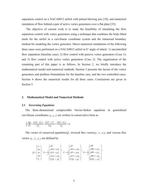
separation control on a NACA0012 airfoil with pulsed blowing jets [19], and numerical simulation of flow behind a pair of active vortex generators over a flat plate [33]. The objective of current work is to study the feasibility of simulating the flow separation control with vortex generators using a technique that combines the body-fitted mesh for the airfoil in a curvilinear coordinate system and the immersed boundary method for modeling the vortex generator. Direct numerical simulations of the following three cases were performed on a NACA0012 airfoil at 6° angle of attack: 1) uncontrolled flow separation (baseline case); 2) flow control with passive vortex generators (Case 1); and 3) flow control with active vortex generators (Case 2). The organization of the remaining part of this paper is as follows. In Section 2, we briefly introduce the mathematical model and numerical methods. Section 3 presents the layout of the vortex generators and problem formulations for the baseline case, and the two controlled cases. Section 4 shows the numerical results for all three cases. Conclusions are given in Section 5. 2. Mathematical Model and Numerical Methods 2.1 Governing Equations The three-dimensional compressible Navier-Stokes equations in generalized curvilinear coordinates ( ξ , η, ζ ) are written in conservative form as ( E E ) ( F F ) ( G G ) 1 ∂ Q ∂ − v ∂ − v ∂ − v + + + = 0 J ∂t ∂ξ ∂η ∂ζ The vector of conserved quantitiesQ , inviscid flux vector ( E , F , G ) , and viscous flux vector ( E , F , G ) are defined by v v v ⎛ ρ ⎞ ⎜ ⎟ ⎜ ρu ⎟ Q = ⎜ ρv ⎟ ⎜ ⎟ ⎜ ρw⎟ ⎜ ⎟ ⎝ Et ⎠ , ( ) ⎟⎟⎟⎟⎟⎟⎟ ⎛ ρU ⎞ ⎜ ⎜ ρUu + pξ x 1 ⎜ E = ⎜ ρUv + pξ y J ⎜ ρUw + pξ z ⎜ ⎝U Et + p ⎠ , ( ) ⎟⎟⎟⎟⎟⎟⎟ ⎛ ρV ⎞ ⎜ ⎜ ρVu + pη x 1 ⎜ F = ⎜ ρVv + pη y J ⎜ ρVw + pη z ⎜ ⎝V Et + p ⎠ 5 , ( ) ⎟⎟⎟⎟⎟⎟⎟ ⎛ ρW ⎞ ⎜ ⎜ ρWu + pζ x 1 ⎜ G = ⎜ ρWv + pζ y J ⎜ ρWw + pζ z ⎜ ⎝W Et + p ⎠ ,
⎛ ⎞ ⎜ 0 ⎛ ⎞ ⎟ ⎜ 0 ⎛ ⎞ ⎟ ⎜ 0 ⎟ ⎜τ ⎟ xxξ x + τ yxξ y + τ zxξ z , ⎜τ ⎟ xxη x + τ yxη y + τ zxη z , ⎜τ ⎟ xxζ x + τ yxζ y + τ zxζ z , 1 ⎜ ⎟ 1 ⎜ ⎟ 1 ⎜ ⎟ Ev = ⎜τ xyξ x + τ yyξ y + τ zyξ z ⎟ Fv = ⎜τ xyη x + τ yyη y + τ zyη z ⎟ Gv = ⎜τ xyζ x + τ yyζ y + τ zyζ z ⎟ J ⎜ ⎟ J ⎜ τ xzξ x + τ yzξ y + τ zzξ ⎜ ⎟ J z ⎟ ⎜ τ xzη x + τ yzη y + τ zzη ⎜ ⎟ z ⎟ ⎜ τ xzζ x + τ yzζ y + τ zzζ z ⎟ ⎜ ⎟ ⎝Q xξ x + Qyξ y + Qzξ ⎜ ⎟ z ⎠ ⎝Q xη x + Qyη y + Qzη ⎜ ⎟ z ⎠ ⎝Q xζ x + Qyζ y + Qzζ z ⎠ where ∂( ξ , η, ζ ) J = is the Jacobian of the coordinate transformation between the ∂( x, y, z) curvilinear ( ξ , η, ζ ) and Cartesian ( x y, z) , frames, and ξ x , ξ y , ξ z , η x , η y , η z , ζ x , ζ y , ζ are z coordinate transformation metrics. ρ is the density. The three components of velocity are denoted by u , v , and w . E is the total energy given by t E t p 1 = + ρ γ −1 2 2 2 2 ( u + v + w ) . The contravariant velocity components U , V , W are defined as U ≡ uξ + vξ + wξ x V ≡ uη + vη + wη x W ≡ uζ + vζ + wζ x y y y z z , z , . The terms Q x , Qy , Q in the energy equation are defined as z Q = −q + uτ + vτ + wτ x y x Q = −q + uτ + vτ + wτ z y Q = −q + uτ + vτ + wτ z xx xy xz xy yy yz xz yz zz , , ; The components of the viscous stress tensor and heat flux are denoted by τ , xx τ , yy τ , zz τ , xy τ , xz τ , and yz q , x q , q , respectively. y z In the dimensionless form, the reference values for length, density, velocities, 2 temperature, pressure and time are L , r ρ , r U , r T , r ρ rU , and r r r U L / , respectively, where the subscript “r” denotes the reference quantities. The dimensionless parameters, including 6
Page 1 and 2: Numerical Study of Passive and Acti
Page 3 and 4: Keywords: flow separation, passive
Page 5: flat plate [34, 35]. Other experime
Page 9 and 10: Viscous terms are taken into accoun
Page 11 and 12: velocity. The negative value is sho
Page 13 and 14: Fig. 5. Streamline of steady flow p
Page 15 and 16: (Case 2), the motion of two vortex
Page 17 and 18: Angle of attack α 6° 4. Numerical
Page 19 and 20: airfoil is shown in Fig. 14. The ne
Page 21 and 22: (a) streamwise vorticity (dark colo
Page 23 and 24: (a) x = 0.163C 22 (b) x = 0.217C Fi
Page 25 and 26: Fig. 20. Mean pressure coefficient
Page 29 and 30: at x = 0.217C shows a wave packet w
Page 31 and 32: of the airfoil at this angle of att
Page 35 and 36: I x = 0.312C 5. Concluding Remarks
Page 37 and 38: cylinder using the immersed boundar

Numerical Study of Passive and Active Flow Separation Control ...

Create successful ePaper yourself

Delete template?

Save as template?