e?Lx:>cP\^l - University of Utah

t 

t 

e?Lx:>cP\^l 

HEAT FLOW AND GEOTHERMAL POTENTIAL OF KANSAS 

by 

David D. Blackwell 

and 

John L. Steele 

Department of Geological Sciences 

Southern Methodist University 

Dallas, Texas 75275 

Final Report 

for 

Kansas State Agency Contract No. 949 

March, 1981

i 

*• 

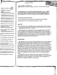
HEAT FLOW AND GEOTHERMAL POTENTIAL OF KANSAS 

ABSTRACT 

Temperature, thennal conductivity measurements and heat flow 

values are presented for fovir holes originally drilled for water 

resovirces investigations bythe D.S. Geological Survey. These holes 

cut most of the sedimentary section and were cased and allowed to 

reach tenperature equilibrium. Several types of geophysical logs 

were also run for these holes. Temperature data from an additional 

5 wells are also presented. Temperature gradients in the sedimentary 

section vary over a large range (over 4:1), and there are significantly 

different temperatures at the same depth in different portions of the 

state. Tanperatures as high as 34"c occur at a depth of 500 m in 

the south-central portion of the state and 28*C or lower in other peurts 

of the state. In addition to cuttings measurements, thermal conductivities 

were estimated fron geophysical well log parameters; the results are 

useful and more use of the technique is suggested. Using these results 

geophysical well logs can be used to predict temperatures as a function 

of depth in areas for which no temperatures are available if heat flow 

is assumed. The extreme veiriation in gradients observed in the holes 

occur because of the leurge contrast in thermal conductivity values. 

Shale thermal conductivity values appeeu: to have been overestimated in 

the past and the Paleozoic shales in Kansas have thermal conductivity 

values of about 1.18 ± 0.03 Whi"lK"l. On the high side, evaporite and 

dolomite units have thermal conductivities of over 4 Wta~^K~i. In spite 

of the large variations of gradient the heat flow values i throughout the

holes do not vary more then 10% and any water flow effects which might 

be present due to the lateral motion on any of the aquifers are less 

than 10%. The best estimates for heat flow in the four holes come 

from the carbonate units below the base of the Pennsylvanian and the 

values range from 48 mWtn~2 to 62 mWta~2. Two of the holes were drilled 

to basement and correlation of the heat flow with the basement radio 

activity suggest that the heat flow-heat production line postulated 

for Midcontinent by Roy et al^ (1968a) applies to these data. Because 

of the low thermal conductivity of the shales the radiogenic pluton 

concept should apply to the Midcontinent. Thus if very radioactive 

plutons can be identified, much higher temperatures may occvur in the 

sedimentary section then has been thought possible in the past. However, 

the past overestimation of shale conductivity values suggests that 

some previous high heat flow values in the Midcontinent are probably 

not correct and the high gradients are merely due instead to normal heat 

flow and very low thermal conductivity values. In spite of its presence 

in the Midcontinent region there could be significant use of geothermal 

energy in Kansas for space heating, thermal assistemce and heat pump 

applications because the temperatures in the sedimentary section in much 

of Kansas are in excess of 40'C.

INTRODUCTION 

At the present time there are only two published heat flow 

measurements available for the state of Kansas. A value of 63 mWhi 

was measured near the central part of the state at Lyons, Ksmsas 

(Sass et al., 1971a) and a value of 59^- mWlm"^ was estimated for a 

site near Syracuse by Birch (1947). In addition a heat flow value 

of 59 inWln"^ was published by Roy et al. (1968b) for a site in extreme 

northeastern Oklahoma near the Kansas border. On a regional basis 

the eastem part of Kansas should be part of the Central Stzdsle 

Region, an area of the North American continent characterized by a 

single linear relation between heat flow and heat production (Roy et aX, 

1968a). In this area, unless heat flow values are disturbed, they are 

directly related to the heat production of the basement underlying the 

site where the heat flow measurement was made. 

There is a suggestion from regional data that heat flow may increase 

toward the west in the Great Plains province and that the high heat flow 

characteristic of the southern Rocky Mountains may extend east of the 

mountains some distance (Blackwell, 1969; Combs and Simmons, 1973; see 

Lachenbruch and Sass, 1977; Blackwell, 1978). Extensive thermal studies 

are in progress in the state of Nebraska but the results are preliminary 

at this time (Gosnold, 1980). Heat flow values may be quite high in 

the western part of the state. Swanberg and Morgan (1979) published a 

heat flow map for the United States based on a correlation of heat flow 

and silica water temperatures. In this map they have a data gap for the 

state of Kcmsas, but extrapolation from data outside the state implies

that the heat flow may be greater than 65 mWta"^ in the western part 

of the state and less than 65 mWm~2 in the eastern part of the state. 

While no heat flow measurements were made as part of this study in 

western Kansas in the area presumed to be characterized by heat flow 

above that characteristic of the Central Stable Region, the data 

presented here do bear on the heat flow values in the Great Plains and 

this topic will be discussed in a subsequent section. 

The plan of the U.S. Geological Survey to drill four deep hydro- 

logic tests in Kansas prompted Dr. Don Steeples to propose a geothermal 

study in these wells; this study has been carried out by the authors 

of this report. These wells offer a unique opportunity to make detailed 

and accurate heat flow measurements in Kansas. These wells were drilled 

through the Arbuckle Group to within a few feet of basement and two 

of the holes were deepened on into the basement ^nd core samples collect 

ed of the basement rock. Because of the depth of the four holes and 

because of the fact that they have been cased through most of their 

depth and left undisturbed to reach temperature equilibrium, it is 

possible to get highly accurate, stable temperature measurements through 

the complete sedimentary section. This opportunity does not arise 

very often in the Midcontinent in spite of the fact that thousands of 

wells have been drilled there, because most of the holes were drilled for 

petroleum exploration and are not available for equilibrium temperature 

studies. Water wells are usually somewhat shallower and thus do not cut 

nearly as thick a section or approach the basement; furthermore possible 

circtdation effects may disturb the temperatures within the wells. In

addition an extensive suite of geophysical logs were obtained for 

each of the holes (gamma-ray, travel time, density, neutroji porosity, 

electric, etc) and cuttings were collected at frequent intervals. The 

holes which were drilled to the Arbuckle Group or deeper by the 

U.S. Geological Survey are 12S/17E-13bbd, 13S/2W-32ccc, 18S/23E-18dcd 

and 31S/20E-22cac. In addition 5 other holes were logged as part of 

this study. For these holes cutting samples and geophysical logs 

are not available, but the additional holes offer useful supplementary 

information on the temperature regime in other parts of Kansas.

MEASUREMENT TECHNIQUES 

The holes were logged to a maximum depth of 1045 m with a truck 

mounted logging system or to 565 m with portable hand operated equip 

ment. Most of the holes were logged with a digital recording system 

attached to the output of the digital volt meter attached to a thermistor 

probe and the output of a digital depth encoder. Temperattures were 

calculated from the measured resistance values and gradients were 

calculated using the two data sets. Temperatures were measured to 

the nearest 0.001°C at depth intervals of 1 m, allowing a very 

detailed look at gradients in the sedimentary section. Logging rates 

were quite slow, 4 m per minute, so that equilibrium temperatures were 

obtained. Roy eib al. (1968b) and many subsequent authors have illustrated 

the detail which can be obtained in sedimentary rocks using such 

continuously recording equipment. The detailed temperature measurements 

are listed in Appendix A along with temperature-depth curves for each 

hole logged. 

Thermal conductivity measurements were made on cuttings from three 

of the holes drilled by the U.S. Geological Svirvey. These results are 

given in Appendix B. Only cuttings were available for the sedimentary 

section so the measurements were made using the chip technique of 

Sass et al. (1971b). Core samples were available frcsn basement rock at 

two of the sites and heat production and thermal conductivity were 

measured on the core samples. These data will be discussed below. Heat 

production measurements were made using a 256 channel gamma-ray pulse- 

height analysis system (Gosnold, 1976). Core sample thermal conductivity 

measurements were made using conventional divided-bar techniques (Roy et aL, 

4 '

1968b). A major problem arose in the use of the chip technique to 

measure thermal conductivities for some of the units in the sedimentary 

section. Because of the strong anisotropy of the layered silicates 

making up the shales it proved impossible to obtain the correct in situ 

thermal conductivity values of the shales using cutting samples. In 

preparing the cylinders with the mixture of water and cuttings it 

appears that many of the fragments of shale will end up randomly 

orientated whereas of course in the gro\ind the orientation is strongly 

preferred. The result is that the calculated ixi situ conductivity 

is far too high; this point is discussed in much more detail below. 

In the tables showing interval thermal conductivity values, these 

values have been corrected for temperature effects in- the deeper parts 

of the holes. These effects approach 0.15 Wm K for the bottom part 

of hole 13S/2W-32CCC (see Robertson, 1975).

GEOTHERMAL GRADIENTS 

Geothermal gradients were obtained in 10 relatively deep holes 

(375 - 1045 m) throughout the eastern 2/3 of the state of Kansas. In 

all of these holes the temperatures as a function of depth show a very 

close relationship to lithologic variations. Because of this corre 

lation and the typically thin individual beds characteristic of the 

Pennsylvemian section cut by most of the holes, it is very difficult 

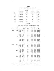
to generalize the results. The hole locations and pertinent information 

are shown in Table 1 and on Figure 1, a generalized index map of 

Kansas. The holes will be individually discussed preceding in order 

from northwest to southeast. All of the data have been plotted on the 

same depth, temperature and gradient scales to facilitate comparisons 

from hole to hole. The deeper holes have been plotted on two depth 

scales, 0-600 eind 500-1100 m to increase the resolution and allow full 

page plots of the shallower holes on the same scale as the deeper holes. 

Bar graphs of gradient are shown for each hole. For the most detailed 

logs, which were digitally recorded, temperatures are plotted at 2 m 

intervals. 

Figure 2 shows a detailed temperature-depth curve and bar graph 

of gradient for hole 9S/20W-27bdc in Rooks County. This hole was 

logged to the end of our cable at 1045 m. The upper part of the hole 

cuts Cretaceous rocks overlying a relatively thick Permian section. The 

units which are most clearly identifiable on the temperature-depth and 

gradient plots in Figures 2a and 2b are the shales. The water table 

was just above 100 m and the first reliable gradients are below 105 m.

TABLE 1. Location data for holes logged. 

Township/Range 

-Section 

9S/20W-27bdc 

12S/17E-13bbd 

13S/ 2W-32CCC 

18S/23E-18dcd 

198/ 8W-23 * 

19S/ 8W-26 * 

25S/ 4E-34dad 

253/ 8E-36acc 

25S/13E-24add 

30S/24E- 2ddd 

31S/20E-22cac 

North 

Latitude 

39°14.7' 

39°00.8' 

38°52.3' 

38''28.6' 

38°23.0' 

38"'22.0' 

37°49.8' 

37°50.0' 

37»51.6' 

37°27.4* 

37°19.8' 

Data from Sass et al. (1971). 

West 

Longitude 

99°32.6' 

95°28.7' 

97°34.5' 

94»54.3' 

98°10.0' 

98°10.0' 

99°58.3' 

96°28.6' 

95°55.4' 

94°44.5' 

95°12.4' 

Hole Name 

Rooks Co. 

Big Spgs. 

Smokyhill 

Watson-1 

LK-1 

LK-2 

Butler Co. 

Sallyard 9 

T.E. Bird 

Frontenac 

USGS-Bst 

Date Logged 

11/15/80 

6/ 5/80 

6/ 5/80 

1/ 9/80 

11/17/70 

11/17/70 

11/19/80 

11/19/80 

11/18/80 

1/10/80 

6/ 4/80 

Collar 

Elevation 

689 m 

365 m 

369 m 

256 m 

525 m 

512 m 

405 m 

402 m 

308 m 

289 m 

285 m 

Depth 

Logged 

1045 m 

565 m 

1044 m 

385 m 

229 m 

328 m 

737 m 

384 m 

441 m 

340 m 

550 m

. J - . . 

4._._4. 

Syracuse 

i^ 

FIGURE 1. 

! 

I 

i 

n- •r"- 

^• 

h—4' 

I 

I- 

I 

4—-1- 

y-y—y- 

I3S/ 2W-^ccc 

--! i 

! i ! i 

! l9S/8W-26^ i 

.,- L,....l i 

I I-X.-J """ 

1 \ -i 

I 

r- 

i i 

i ! 

I I 

0 

L 

KM 

i, RS/l7E-(3bbd D U.T- 

i 

I* 

•T—•? i - r 

l8S/23E-l8dcdr> 

i ^ !-- 

I ^1 

! _25s/8E-36ac9 

253/ 4'e-34dado JO b J 

: 25S/l3E-24oddi , 

r- 

/ 

I 

r 

I i30S/24E- 2dddo 

! i j—oi 

r'3lS/l0E-22cac 

Index map of sites of published heat flow values (solid circles) and sites of holes 

discussed in this report (open circles). 

IOO 

1 

I 

CO

cn 

cc 

LU 

LU 

LU 

Q 

100 

200 

300 

400 

500 

600 

.12 

TEMPERfiTURE, OEG C 

16 20 24 28 

— I — I — I — I — I — I — I — I — I — I — I — f 

I .1 r I L-J I 

T 1 1 1 1 1 T 

K 9S/20H-27BDC 

U/15/80 

GRflD., DEG C/KM 

FTfiiiRF. ?A- Temperature-depth and gradient-depth curves for hole 9S/20W-27bdc. Two-meter gradient 

intervals are plotted. ' ' •• 

ô

a-) 

D: 

ijj 

\— 

u I 

2; 

Q. 

UJ 

Q 

TEMPERfiTURE, DEG C 

500 .24 28 32 36 40 

T—I—I—p£i—r—r T—I—r 

600 

700 

800 

900 

1000 

1100 

% 

% 

%. 

% 

T T—r ""^ T—I—r 

44 

* 9S/20W-27BDC _ 

11/15/80 

GRRD., DEG C/KM 

' I I U_J I I I I L I I I I I I L J I ' I ' L 

FIGURE 2B. Temperature-depth and gradient-depth curves for hole 9S/20W-27bdc. Two-meter gradient 

intervals are plotted. 

70

There a section 60 m thick between 105 m and 165 m has a mean gradient 

of 50.5 ± 0.3"c/km. Below that section the gradient drops to approximately 

37.5 ± 0.5''C/kmto a depth of 221 m at which point the gradient drops 

to values generally less tham SO'c/km, which continue to the bottom of 

the hole. The only exception is a zone of higher gradient between 

300-340 m and a few local intervals of higher gradient between 900 and 

1000 m. The Cretaceous-Permicui unconformity is at a depth of about 

450 m and the Pennsylvanian-Permian contact is at a depth of approximately 

900 m in this hole. The mean gradient in the Cretaceous section 

(105-450 m) is 27.3 ± 1.8*C/km. In the Permian section (450-900 m) the 

mean gradient is 24.2 ± O.S'C/kmand in the Pennsylvanian section (900- 

1045 m) the mean gradient is 33. 6 ± 0.3°C/km. In the Pennsylvanian section 

the gradients are variable ranging from 45°C/km in the predominantly shale 

units to 25°C/km in the more limestone rich units. Temperatures 

are somewhat lower in this hole then in most of the other holes logged, 

either because of a higher thermal conductivity for the Permian section, 

which includes more sandstone and evaporite deposits than the Pennsylvanian, 

or because of a lower heat flow at this site than at the remainder of 

the sites. The thermal conductivity hypothesis is favored. 

Hole 12S/17E-13bbd, although drilled into Precambriah basement at 

a depth of 910 m, was logged only to a depth of 565 m. A second attempt 

was made to log the hole to total depth, but it was being used by the 

U.S. Geological Survey and was inaccessible. The temperature-depth 

data and a bar graph of gradient for this hole are shown in Figure 3. 

The gradient in the Pennsylvanian section between 120 m and 521 m ranges 

11

CO 

DC 

LU 

l_ 

LU 

a. 

LU 

Q 

100 

12 

0 

200 - 

300 

400 

500 

600 

TEMPERATURE, DEG C 

16 20 24 28 

1—J—I—j—I—I—I—I—I—I—I—j—I—I—I—I—I—I—r 

« 12S/17E-13BBD 

6/ 5/80 

I ' « ' « 1 L_l « « ' ' ' I L 1-J. J L 

32 


T—I—n r—I—r 

^ 

T_ 

2. 

^ 

t=5: 

^ 

7=^ 

J I I I I L 

FIGURE 3. Temperature-depth and gradient-depth curves for hole 12S/17E-13bbd. Five-meter gradient 

70

from 25'*C/km to just over 40'*C/km and averages 32.1 ± 1.0°C/)an. In 

the Pre-Pennsylvanian carbonate section below 520 m(to 565 m) the mean 

gradient is 17.1 ± 0.1°C/km. 

Temperature-depth curves and bar graphs of gradient for hole 

13S/12W-32CCC are shown in Figure 4. This hole was drilled for the 

U.S. Geological Survey to a depth of 1117 m and was logged to a depth of 

1044 m. The stratigraphic section in the upper part of this hole is 

similar to hole 12S/17E-13bbd; however, temperature data from the 

deeper section were also obtained. When this hole was logged an 

injection test had recently been completed, and in the bottom part of 

the hole the temperatures were unstable, apparently because of this 

test. The gradients averaged over 15 m intervals are fairly character 

istic of those in the rock (see Figure 4c), but the 2 m interval 

gradients are very variable as the hole tends toward equilibrium. 

Some of the injected fluid may have entered the formation around 920 m 

resulting in the very low gradients in that section of the hole. The 

mean gradient between 100 and 280 m in the Permian section is 28.5 ± 

0.6''c/km. The mean gradient in the Pennsylvanian section (280-792 m) 

is 31.9 ± 0.6''c/km. Below 792 m in the Pre-Pennsylvanian section the 

units are more monolithologic and there is a good correlation between 

lithology and gradient (Figure 4c). The section of high gradient between 

558-598 m corresponds to the Lawrence shale. The gradient in this section 

is 48.6 ± 0.1°C/km. The mean gradient between 736 and 796 m in the 

Cherokee shale is 36.9 ± 0.2°G/km while the mean gradient in the 

Chattanooga shale between 862 and 912 m is 52.1 + Cl^C/km. 

13

(T) 

OC 

LU 

h- 

LU 

Q_ 

LU 

a 

100 

200 

300 

400 

500 

600 

J 2 

0 

TEMPERfiTURE, DEG C 

16 20 24 28 

T T 

1—I—r r T—I—I—I—I—I—r 

J I L J__J I I I I I I I 

T—r T—I—r 

)K 133/ 2M-32CCC _ 

6/ 5/80 

32 


T 1—-i r 

- cL P 

5. t—,, 

1 i 

1. c 

- £ ^ 

T 

J I I I L 

10 70 

FIGURE 4A. Temperature-depth and gradient-depth curves for hole 13S/2W-32ccc. Five-meter gradient 

intervals are plotted.

CO 

GC 

LU 

l~ 

LU 

Q. 

LU 

a 

50 cf^ 

600 - 

700 

800 

9D0 

1000 


32 36 40 44 

ran—I—I—I—I—I—I—1—I—I—I—I—I—r 

X IBS/ 2U-32CCC 

11/17/80 

GRAD., DEG C/KM 

1100 r * ' I 1 I • I ' I > « L J I I cn 

FIGURE 4B. Temperature-depth and gradient-depth curves for hole 13S/2W-32ccc. Two-meter gradient 

intervals are plotted. -•—-—=

^ 700 

OC 

LU 

I— 

LU 

O. 

LU 

a 900 

1000 

1100 

TEMP 

DEG C 

32 36 40 

T—I—I—I—I—j—I—I—I—I—I—r 

13S/ 2U-32CCC 

15 POIHT flVERflGE 

44 48 

"]|—I—I—r- 

J I I I I I L-J L-J I L J^-J I I I L 

I I I I 

GRADIENT 

DEG C/KM 

' ' « • ' ' ' ' • » ' ' ' • o> 

35 70 

FIGURE 4C. Temperature-depth and gradient-depth curves for hole 13S/2W-32ccc. Fifteen-meter running 

average gradient values are plotted.

The mean gradient in the limestone units ranges from 15 to 25*'C/km. 

This hole was logged just into the Arbuckle Group (top at 1026 m). 

The detailed geology and heat flow for this hole will be discussed in 

the following section. 

Hole 18S/23E-18dcd was also one of the holes drilled for the 

U.S. Geological Survey. At the time of the first logging it had 

collapsed at 395 ro and we were unable to go deeper; during a second attempt 

to log the hole, the hole was inaccessible due to muddy conditions of 

the surrounding field. We intend to relog this hole when conditions 

allow. The temperature-depth curve and a bar graph of gradient are 

shown in Figure 5. This hole shows generally high gradients,ranging 

between 37 and 57*'c/]cm and averaging 51.08 ± 1.2"C/km,between 100 m and 

220 m, the Mississippian-Pennsylvanian contact. The gradient drops 

abruptly to average 22.7"± 0.7°C/km in the remainder of the hole, with 

the exception of a 15 m section in the Chattanooga shale. The average 

gradient in the Chattanooga shale (360-375 m) is 52.5 +^ 0.1°C/km. There 

is a negative gradient section near the bottom of the hole which reflects 

a drilling or injection disturbance. The mean gradient for the bottom 

of the hole below the Chattanooga shale is only 14.5°c/km although it is 

poorly determined. This section is predominately dolomite as discussed in the 

section on heat flow. The hole was drilled into basement and bottomed 

at 666 m. Basement thermal conductivity and heat production data cure 

discussed below. 

Hole 19S/8W-26 was logged and the data presented by Sass et al. 

(1971a). The temperature-depth and gradient data are shown in Figure 6; 

17

cc 

LU 

LU 

100 

200 

300 

Q. 

LU 

CD 400 

500 

J 2 

TEMPERATURE, DEG C GRAD., DEG C/KM 

16 20 24 28 32 

T T 

1 — I — I — I — I — I — I — I — I — I — I — I — I — I — I — I — r 

m 18S/23E-I80C0 > 

1/ 9/80 

500 ' ' ' ' ' ' ' • ^ •- « « ' « ' I L-J I L 

T 1 r—*T 1 r 

«=c 

J I I L 

0 70 

FIGURE 5. Teii5)erature-depth and gradient-depth curves for hole 18S/23E-18dcd. 2.5-meter gradient 


^ 

00

(Ji 

cc 

LU 

H- 

LU 

CL 

LU 

Q 

100 

200 

300 

400 

500 

600 

12 

0 


16 20 24 28 

T — I — I — I — I — I — I — J — I — I — I — I — I — I — I — I — I — I — r 

3K 195/ 8H-26 

11/17/70 

» ' ' ! ' ' ' I I I ' ' ' ' I I I I L 

32 


T 1 1 r 

5" 

• - - ^ 

Z^ 

Iz. 

^ 

J L J L_-J I 

70 

FIGURE 6. Temperature-depth and gradient-depth curves for hole 19S/8W-26 (Sass et al., 1971a). 

^

this hole was drilled in Permian age rocks with the section of the 

hole between 220 and 305 m in salt deposits. Because of the high 

thermal conductivity of the salt a low gradient of only 14''c/km is 

observed within this interval. 

Three holes were logged along a more or less east-west section 

in south center part of the state, holes 25S/4E-34dad, 25S/8E-36acc and 

25S/13E-23add. These holes are predominately in Pennsylvanian age 

rocks and have the highest temperatures in the 400-500 m depth range 

observed in any of the holes logged. In large part the high temperatures 

are due to the greater abundance -of shale of low thermal conductivity in 

the geologic section encountered in these holes. The temperatvure-depth 

curves and bar graphs of gradient for the first two holes are shown in 

Figures 7a and 7b and 8. The mean gradient for hole 25S/4E-34dad 

between 200 and 737 m is 35.6 ± ce'c/km. The gradients for 25S/4E-34dad 

are quite variable; this hole was an abandoned oil well and some of 

the irregularity may be related to past production effects. The character 

of the gradient variations changes abruptly at 310 m. At this point 

a ball of mud or some other material apparently attached itself to the 

probe severely lengthening the time constant of the probe and resulting 

in the marked change in behavior. The fluid level in hole 25S/8E-36acc 

was at 195 m and logging did not begin until below that depth. The mean 

gradient for that hole is 38.0 ± 0.4''C/km between 200 and 390 m. 

A temperature-depth cuirve and a gradient bar graph for hole 

25S/13E-24add are shown in Figure 9. In this hole there is a variation 

of 10-20 m interval gradients from about 25 to 55''c/km. From a comparison 

20

(n 

cc 

LU 

zc 

h- 

DL 

LU 

a 

100 

200 

300 

400 

500 

600 

J 4 


18 22 26 30 

T T—I—r M ' ' I T—I—I—j—I—I—r 

34 

* 255/ 4E-34DRD - 

11/19/80 

' ' ' i L—I I I I I I I 1 1 L J L 


0 35 70 

FIGURE 7A. Temperature-depth and gradient-depth curves for hole 25S/4E-34dad. 


Two-meter gradient 

to

CO 

CE 

UJ 

h- 

LU 

rc 

I— 

d. 

LU 

a 

50(?« 

600 

700 - 

800 

900 - 

1000 

1100 


40 44 48 

-i—I—J—I—I—I—I—I—I—r 

* 253/ 4E-340flO 

11/19/80 

J I L J I L J I L J I I J I I 


I I I I I I an I I I I I 

« ' ' I I I ' I I I ' I I 

35 70 

FIGURE 7B. Temperature-depth and gradient-depth curves for hole 25S/4E-34dad. Two-neter gradient 


to

CO 

CE 

LU 

h- 

LU 

CL 

LU 

Q 

100 

200 

300 

400 

500 

Ol I I 1 

600' ' ' ' 


16 20 24 28 

T—I—r T T — I — I — I — I — I — I — I — I — r 

« 255/ 8E-36flCC 

11/19/80 

I I I I I I. I I I I I I J I L 

32 


T 1 1 1 1 r 

' I ' I I.. I 

0 70 

FIGURE 8. Temperature-depth and gradient-depth curves for hole 25S/8E-36acc. Two-meter gradient 

intervals are piottea. '—'—'—' —.—-= - 

(O

CO 

cc 

LU 

\— 

LU 

CL 

LU 

Q 

100 

200 

300 

400 

500 

14 

0 

TEMPERATURE, DEG C GRAD., DEG C/KM 

18 22 26 30 34 

mn*—I—I—I—I—I—I—I—I—I—I—I—I—I—I—I—I—r 

nn 25S/l3E-24flOD _ 

11/18/80 

\ " 

I I I I I I r I I I I I 

600 L-J I L-J L_J L-J—J I I I I I I I I I I I I I I I I I I i I I I I I 1 I 

0 35 70 

FIGURE 9. Temperature-depth and gradient-depth curves for hole 25S/13E-24add. Two-meter gradient 

xntervals are plotted. 

^-E 

to

with the gamma-ray log it is clear that these high gradients are closely 

correlated with sections of the hole which have higher gamma-ray 

activity, i.e., the shale sections. The sections of lower gamma-ray 

activity are predominately limestone although there may be some sand 

stone represented by lower gamma-ray activity as well. The contacts 

between the shales and limestones appear quite sharp on the gamma-ray 

log above 150 m and not so sharp on the temperature log below 150 m. 

This may be due to mud collecting on the probe and increasing the time 

constant, because this long time constant type behavior is not observed 

in the other holes logged (except hole 25S/4E-34dad, see above) or in 

the upper part of this hole. The mean gradient for the hole between 

40-441 m is 42.2 ± O.g'C/km. 

The only water well logged was hole 30S/24E-2ddd. This hole was 

logged to a depth of 340 m. The temperature and gradient data are 

shown in Figure 10. Because the hole is an abandoned water well the 

gradients may be disturbed by water circulation. From the shape of the 

temperature-depth curve there appears to be borehole upflow between the 

bottom and about 220 m. Not much is known of the section in this hole, 

but it is probably predominantly carbonate. The temperatures are quite 

low probably because it is one of holes furthest to the east where the 

Pennsylvanian section is thinnest. The mean gradient between 105 and 

340 m is 19.7 ± l.e'c/km. 

Extensive data are available for hole 31S/20E-22cac, one of the 

holes drilled by the U.S. Geological Survey. This hole was logged to 

the drilled depth of 550 m (1804 ft.). The results are shown in Figure 11. 

25

CO 

cc 

LU 

LU 

CL 

LU 

Q 

100 

200 

300 

400 

500 

600 

_12 


16 20 24 28 

T 1 1 1—I 1—T T r-T—I—I—I—r T 1—I—r 

m 30S/24E- 2000 

1/10/80 

J I I I I I ' I I I ' J L . I l.l .1 

32 


I I I I I I I I I I I I I 

:Z 

' ' ' ' ' ' ' « ' ' ' ' ' 

35 70 

FIGURE 10. Temperature-depth and gradient-depth curves for hole 30S/24E-2ddd. 2.5-meter gradient 


to 

(Tt

CO 

GC 

LU 

1— 

LU 

CL 

LU 

Q 

100 

200 

300 

400 

500 

600 

0 12 

1—I—r 

TEMPERATURE, DEG. C 

16 20 24 28 32 

n—j—I—I—I—j—I—I—I—I—I—I—r- 

» 3lS/20E-22CflC _ 

6/ 4/80 

O 31S/20E-22CflC - 

11/19/80 

' • ' J I L J L . I . J I L 


I I I I I I j I I I I I I 

i 

- ^ 

s=? 

' ' ' ' ' ' ' ' 

35 

FIGURE 11. Temperature-depth and gradient-depth curves for hole 31S/20E-22cac. Five-meter gradient 

int-oruala ffre> p^^^*-t•pf\, 

y=' 

^ . 

I ' ' 

70 

to

The gradients between 95 m and 205 m are quite high, averaging 

53.4 ± 1.5"c/km. Below 205 m the gradients average less then 20''C/km. 

The 205 m depth is the contact of the Pennsylvanian section with the 

predominantly limestone-dolomite section of Mississippian and older 

age. At the bottom of the hole there are two negative temperature 

excursions which are related either to drilling, to injection, or 

to some small water flow existing in the hole previous to drilling. 

Because of the thinness of the high thermal conductivity section, 

temperatures at depth are relatively low in this hole. 

Using the data obtained directly from the logs a table of 

temperatures at various depths was prepared and is shown in Table 2. 

Temperatures are shown at depths of 400, 500, 750 and 1000 m 

where available. Extrapolations have not been made except for very 

short depth intervals. Where extrapolations have been made the nximbers 

are given in parentheses. Most of the holes were logged to a depth 

of 400 m but only about 2/3 of then are logged to a depth of 500 m. 

A contour map of temperature at 500 m is shown in Figure 12. At this 

depth temperatures are highest in the southern third of the state except 

along the Missouri boundary. Temperature differences approach e^C 

at a depth of 500 m. The mean surface temperature for almost all of 

the stations is between 13 and 15"C and thus the mean greuJients to 

500 m range from approximately 40'*C/km in the areas of highest 

temperature to only 28''c/km in the north-central portion of the state. 

However, these gradients cannot necessarily be projected to 

greater depths. It is clear that vertical gradient variations are 

28

TABLE 2. Temperatures CO measured at selected depths. Extrapolated 

tenêratures are in parentheses. 

Location 

9S/20W-27bdc 

12S/17E-13bbd 

13S/ 2W-32CCC 

18S/23E-18dcd 

19S/ 8W-26 

25S/ 4E-34dad 

25S/ 8E-36acc 

25S/13E-24add 

30S/24E- 2ddd 

31S/20E-22cac 

0 

(14.0) 

13.9 

14.0 

(13.0) 

15.0 

(14.0) 

(13.0) 

14.0 

(15.0) 

15.0 

400 

26.2 

25.7 

25.8 

27.3 

(25.5) 

28.4 

29.5 

30.8 

25.0 

28.6 

Depth (meters) 

500 

28.4 

29.4 

29.1 

(30.0) 

32.2 

(34.0) 

30.0 

750 

34.2 

37.1 

40.7 

1000 

41.8 

45.2 

to 

iO

TEMPERATURES AT 500 METERS 

0 

L 

IOO 

FIGURE 12. Isotherms at 500 meters. Temperatures are in °c. 

KM 

30,0 

o

due to lithology and so very large variations in gradient will occur 

with depth. Fiirthermore there may be variations of heat flow related 

to other factors such as basement radioactivity. In order to evaluate 

some of these other variations,heat flow values were calculated for 

several of the holes. These heat flow values are discussed in the 

following section. 

31

HEAT FLOW 

Heat flow values have been calculated for the four holes drilled 

by the U.S. Geological Survey. Thermal conductivity measurements were 

made on cutting samples collected from 3 of the 4 holes. The detailed 

results of the measurements are contained in Appendix B. Suites of 

geophysical logs were run in all four of the holes, so log data were 

available to calculate the average iji situ porosity for correction of 

the bulk thermal conductivity to the i^ situ thermal conductivity. The 

gradient segments chosen for averaging were selected from comparison 

of the temperature-depth logs discussed in the previous section to the 

geophysical logs and the geological analysis of cuttings from the wells. 

In most cases there is very good correlation between the gradient 

and lithology, although in the Pennsylvanian section there is such a 

rapid vertical variation of lithology that in most cases the temperature 

data are not detailed enough to be identified with the individual units. 

This rapid vertical variation leads to difficulty in calculating heat 

flow because it is almost impossible to isolate intervals composed only 

of one lithology over which heat flow values can be reliably calculated. 

Where temperatures were measured in the Mississippieui and older carbonate 

section, the. thicker monolithologic units are suitable for heat flow 

calculations and the most reliable values come from these sections of the 

drill holes. The data for interval gradient, harmonic average thermal 

conductivity, and heat flow for each of the four holes are shown in 

TaQjles 3 through 6. Generalized lithology for each of the intervals is 

also listed. In general the mean gradients in the carbonate sections of 

32

all the holes sure almost identical, averaging 20 to 2l''C/km in sections 

which are predominantly limestone and 14 to 17'*C/km in sections which 

include dolomite. Gradients in the predomincintly shale sections range 

from 35 to 53''C/km. 

The results of interval geothermal gradient and heat flow calcula 

tions for hole 12S/17E-13bbd are shown in Table 3. Unfortunately only 

a short section of temperature data in the carbonate section, below 

520 m, is available 2md thus the gradient is poorly determined. Consequently 

the heat flow calculated for that interval, 48 mWln~2, is poorly determined. 

The heat flow values calculated in the upper section of the hole are 

much higher. This situation is discussed in the following paragraphs. 

The results for hole 13S/20W-22ccc are shown in Table 4. Heat flow 

values calculated for the various carbonate sections range from 49-60 mWm""^ 

and average 57 mWm"^. As was the case for hole 12S/17E-13bbd the heat 

flow values in the upper sections of the hole are significantly higher. 

However, in hole 13S/20W-32ccc the Chattanooga shale has 

a gradient of 52.2'*C/km and an apparent heat flow of 124 mWta-2, between 

carbonate units with gradients of 17 and 20°C/fem and heat flow values of 

49-60 mWhi"^, The Sylvan shale section has a gradient of 46''C/km and an apparent 

heat flow of 98 mWhi~2 with the carbonate units on either side having 

gradients of 17.3 and 21.0''c/km and heat flow values 49 and 58 mWm"^. since 

the heat flow is the same on either side of these two shale units the only 

conclusion that is consistent with the data is that the thermal conductivity 

of the Chattanooga shale is about 1.1- 1.2 Wn K and the 

conductivity of the Sylvan shale is about 1.3 Wm K . The data for hole 

33

TABLE 3. Interval thermal conductivity, geothermal gradient and heat flow for hole 12S/17E-13bbb. 

The thermal conductivity in column (2) is the value inferred from the best average heat 

flow divided by the gradient for that interval. Standard error listed under values. 

Depth Interval 

meters 

120 - 145 

145 - 165 

165 

180 

260 

315 

520 

— 

- 

- 

- 

^ 

180 

260 

315 

520 

565 

Thermal Conductivity 

JL J- 

8 

15 

BEST HEAT FLOW VALUE 

9 

0.10 

0.10 

0.10 

0.10 

0.06 

Wm~"'"K~ 

(1) 

2.36 

0.10 2.91 

0.10 2.16 

2.23 

0.12 

2.56 

0.10 

2.51 

0.15 

2.79 

0.15 

(2) 

1.17 

1.85 

1.30 

1.64 

1.88 

1.34 

Gradient 

mKm 

41.0 

0.1 

26.0 

0.1 

37.0 

0.1 

29.2 

0.5 

25.5 

0.3 

35.8 

0.4 

17.1 

0.1 

Heat Flow 

mWtn -2 

97 

76 

80 

65 

65 

89.7 

48 

48 

5 

Generalized 

Lithology 

Lawrence Shale 

Predominantly limestone 

Predominantly shale 



Cherokee Shale 

Limestone and dolomite

TABLE 4. Interval thermal conductivity, geothermal gradient and heat flow for hole 13S/2W-32ccc. 

The values included in the heat flow averages are indicated by the asterisks. The thermal 

conductivity in column (2) is the value inferred from the best average heat flow divided 

by the gradient for that interval. Standard error listed under values. 


meters 

110 - 150 

150 - 275 

150 - 455 

455 - 555 

558 - 598 

598 - 634 

634 - 644 

644 - 694 

694 - 710 

710 - 736 

736 - 796 

796 - 862 

862 - 912 

912 - 942 

944 - 970 

970 -1044 


N (t> 

2 

4 

2 

1 

1 

3 

1 

2 

3 

2 

2 

2 

0.16 

0.12 

0.09 

0.09 

0.06 

0.06 

0.09 

0.09 

0.10 

0.06 

0.09 

0.05 

Wm" K~ 

(1) 

1.93 

2.20 

0.15 

2.44 

2.25 

2.60 

2.45 

2.47 

2.31 

2.92 

2.30 

2.82 

2.70 

(2) 

1.17 

1.54 

1.09 

1.25 

Gradient 

mKm 

25.5 

0.3 

29.0 

0.2 

34.4 

1.0 

27.4 

0.3 

48.6 

0.1 

26.9 

0.1 

31.3 

0.1 

27.5 

0.1 

34.6 

0.1 

25.3 

0.1 

37.0 

0.2 

20.4 

0.3 

52.2 

0.1 

17.3 

0.1 

45.5 

0.1 

21.0 

Heat Flow 

r_-2 

mWm 

5 0.06 2.73 

0.25 

57* 

BEST HEAT FLOW VALUE 57 

6 

49 

64 

119 

61 

81 

67 

62 

86 

60* 

120 

49* 

123 

Generalized 

Lithology 

Shale and limestone 

Limestone and shale 



Lawrence Shale 

Limestone 

Conglomerate and shale 

Limestone and shale 


Sandstone 


Mississippian Limestone 

Chattanooga Shale 

Hunton Group 

Sylvan Shale 

. 

Viola & Arbuckle.Group 

Ul

18S/23E-18dcd are shown in TeJsle 5. The heat flow calculated for the 

carbonate section is 60 mWta~2. The gradients in the Cherokee Shale 

and Chattanooga Shale are 52*'C/km and the directly calculated heat 

flow values are over 110 mWta~2. The heat flow on either side of the 

Chattanooga Shale is identical. If the true thermal conductivity for 

these two units is 1.15 ± 0.5 Win~lK~l then the heat flow in the shale 

units would be the same as in the carbonate units. 

The data for hole 31S/20E-22cac are shown in Table 6. Thermal 

conductivity measurements were made on samples from the Arbuckle Group. 

The rock is a dense dolomite with a high thermal conductivity so that 

even though a large interval (290-550 m) has a low gradient, the heat 

flow is the highest (by only 3%) of all the values obtained. The 

gradients are slightly higher in the limestone section of the hole 

above the dolomite, and much higher (by a factor of over 4) in the 

Cherokee Shale. The inferred thermal conductivity of the shale is 

shown in parentheses. The gradients in the Arbuckle section are exactly 

the same in this hole and in two holes discussed by Roy et_ al^ (1968b, 

see Decker eind Roy, 1974) , near Picher Oklahoma, about 50 km to the 

southeast. The heat flow values are also similar so that apparently 

the Arbuckle thermal conductivity is very similau: in both holes. The 

heat flow for the holes discussed by Roy (1968b) was based on thermal 

conductivity measurements of core samples from Precambrian basement 

rocks. 

36

TABLE 5. Interval thermal conductivity, geothermal gradient and heat flow for hole 18S/23E-18dcd. 

The values included in the heat flow averages are indicated by the asterisks. The thermal 

conductivity in colvunn (2) is the value inferred from the best average heat flow divided 

by the gradient for that interval. Standard error listed under values. 

Depth Ij nterval 

meters 

100 - 

115 - 

220 - 

297.5 - 

360 - 

375 - 

115 

220 

297.5 

360 

375 

395 


N (j) Wm'^K"""" 

(1) (2) 

7 

6 

4 

2 

9 

0.12 

0.08 

0.12 

0.06 

0.05 

2.25 

0.15 

2.56 

0.25 

3.00 

0.30 

2.24 

3.96 

1.15 

1.14 

Gradient 

mKm 

36.9 

0.1 

52.4 

1.1 

23.2 

0.4 

20.1 

0.2 

52.5 

0.1 

14.5 

0.1 

Heat Flow 

mWm -2 

BEST HEAT FLOW VALUE 60 

3 

115 

60* 

60* 

118 

57* 

Generalized 

Lithology 



Mississippian Limestone 

Dolomite 

Chattanooga Shale 

Dolomite 

OJ

TABLE 6. Interval thermal conductivity, geothermal gradient and heat flow for hole 31S/20E-22cac. 

Thermal conductivity value estimated as discussed in text. Standard error listed under values. 


meters 

70 - 205 

205 - 220 

220 - 240 

240 - 290 


N

On the basis of this analysis there would appear to be only minor 

variation of heat flow between the four holes. The mean value for all 

the carbonate sections ranges from 48-60 mWhi~2. However, if heat flow 

values are calculated from thermal conductivity measurements on cuttings 

from the PrePennsylvanian shale sections or from the Pennsylvanian units 

in each hole then an extremely different pictvire of the heat flow is 

obtained. Typical cuttings determined thermal conductivities for the 

shale sections, assuming porosity measured in^ situ of 10% ± 5%, are 

1.8 to 2.25 Wm'^K"-'-. These values taken together with typical gradients 

of 45 to 55''c/km imply heat flow values in the shale sequences of 100 mWIm"^ 

or greater. These values are in clear contradiction to the heat flow 

values obtained in the carbonate units. 

There are two possibilities for the differences in heat flow in 

the different lithologies. It is possible there is a difference in heat 

flow between the upper and lower parts of the drill holes. One of the 

reasons for drilling the wells was to investigate possible fluid flow 

or} the Arbuckle aquifer and slow fluid motions could change the heat 

flow, resulting in either lower or higher heat flow values above the 

aquifer and also effecting heat flow values below the aquifer. The second 

possiblitity is that the thermal conductivity of the shales is misestimated 

by the chip technique. We will examine these two hypotheses in order. 

According to the first hypothesis there should be a change in heat 

flow associated with the contact between the relatively impermeable shale 

section and the lower, more permeable dominately carbonate section. 

39

There are several arguments against this hypothesis. The first of 

these is that for two of the holes which cut fairly thick sequences 

of Pennsylvanian strata, the variation in geothermal gradient within 

the Pennsylvanian section ranges from 25°C/km to 50*C/km. The lower 

values appear to be in sections which have a higher proportion of 

limestone than the sections with higher gradient. These gradient 

values are about 20% higher then those in the PrePennsylvanian carbonate 

section. Since most of the limestones in the Pennsylvanian section 

are very thin, however, most of these intervals probably include some 

shale. The second major argument against the water flow hyjjothesis 

is the interbedding of the shale and carbonate units with their varying 

gradients. 

The conclusion of this discussion is that range of thermal 

conductivity for at least some of the shales encountered in the holes 

is between 1.1 and 1.3 Wm'^K"^. Thus there is an approximate ratio of 

2'5:1 between the thermal conductivity of the limestone and shale and 

up to 4:1 between the thermal conductivity of dolomite and shale. 

Corresponding ratios of gradients in the various units are observed. 

An examination of the chip technique of thermal conductivity 

measurements indicates that it is not surprising that the shale con 

ductivity will be in error. Since small fragments of shale are packed 

into a hollow cylinder, some of them may be on end and all of them are 

finite in length, therefore conduction along the grains in the high 

conductivity directions may be important. It is very difficult to 

measure thermal conductivity on core samples of shales as well and 

40

perusal of the literature indicates in fact, adequate thermal con 

ductivity measurements for shale may not exist. It is difficult to 

measure shale thermal conductivity on the divided-bar using core 

samples because of the fissility of the shale. The anisotropy makes 

needle probe measurenents of dubious value. In heat flow studies in 

the Midcontinent previous investigators have estimated the conductivity 

of the shale sections between 1.55 and 1.85 Wta"^K~^ (Garland and 

Lennox, 1962; Combs and Simmons, 1973; Scattolini, 1978). Judge and 

Beck (1973) encountered the problem in a study of heat flow in the 

Western Ontario Basin where the rocks range in age from Precambrian 

to Mississippian. They found heat flow values 60% too high in the 

Ordovician shale section (Collingwood Formation). If a value of 

1.1 Wm'^K" is asstmied, as determined above for the lower Paleozoic 

shales in this study, the heat flow in the Collingwood Formation is 

the same as in the remainder of the units they studied (dominantly 

limestone and dolomite). Thus the shale thermal conductivity values 

in the literature are significantly in error. One implication is that 

the heat flow in the Great Plains may not be as high as has been 

estimated in the past. In particular the zone of high heat flow extend 

ing out into the Great Plains north of the Black Hills (Lachenbruch and 

Sass, 1977; Blackwell, 1978) may not in fact, exist. Furthermore, the 

correlation of silica values of groundwater and heat flow for the Mid- 

continent may be instead a correlation of silica values and mean geo 

thermal gradient. 

41

Thus in spite of the large amount of high quality temperature 

data, the conventional heat flow values for the foxir holes must be 

based on only small sections of the hole and large sections of the 

hole csuinot be used for heat flow determinations by conventional 

heat flow techniques. In the next section we will investigate the 

use of well log parameters in conjunction with the temperature data 

in order to more cOTipletely evaluate the best heat flow values for 

these four holes. 

42

CALCULATION OF HEAT FLOW UTILIZING WELL LOGGING PARAMETERS 

Because of the difficulties of evaluating the mean thermal conduc 

tivity in the shale sections and in sections with very rapidly varying 

theinnal conductivity it would be useful to have other techniques to 

evaluate these sections. Since four of the holes had available extensive 

geophysical well log suites the use of these data to assist in calcula 

tion of the heat flow values was investigated. It has been demonstrated 

in a number of studies that of various physical properties such as 

density, porosity and velocity, velocity is most directly useful in estimating 

thermal conductivity (Goss and Combs, 1976; Williams, 1981) so emphasis 

was placed on use of the velocity and gamma-ray logs. The gamma-ray activ 

ity in these holes is relatively directly related to, the amount of shale. 

Typical gamma-ray counts for the shale sections are about 100 ± 25 API 

units, whereas in the carbonate sections gamma-ray values axe 25 ± 5 API 

vinits. If the primary control on the thermal conductivity is the mixing 

of only two lithologies then it should be possible to obtain a good 

correlation between gamma-ray activity and the gradient. 

A series of bar graphs of temperature gradient, gamma-ray activity 

and velocity for the four wells drilled for the U.S. Geological Siirvey 

are shown in Figures 13, 14, 15 and 17. For holes logged with the 

digital equipment, gradient graphs are plotted using a running 2 m 

average except for hole 13S/2W-32ccc where a 15 point running average 

was used because of the problems discussed above. In addition the 

i 

gradient data from hole 25S/13E-24add are accompanyed by damma-ray log 

from a nearby hole (Figure 16). The geophysical logs are based on 

43

^ 200 

LU 

GRADIENT 

DEG C/KM 

GAMMA 

API 

VELOCITY 

KM/SEC 

FIGURE 13. Comparison of geothermal gradient, y-ray activity and P-wave velocity for hole 12S/17E-13bbd. 

The Y-ray and P-wave data are based on 0.5 m digitized well logs smoothed by a 7-point average. 

Gradient plot from Figure 3.

600 

GRflDIENT 

DEG C/KM 

„0 35 70 

01 I I I I I I I I I I I I I 

GRMMfl 

API 

VELOCITY 

KM/SEC 

0 too 200 

FIGURE 14A. Comparison of geotheimal gradient, Y-ray activity and P-wave velocity for hole 13S/2W-32ccc. 

The Y-ray and P-wave data are based on 0.5 m digitized well logs smoothed by a 7-point average. 

Gradient plot from Figure 4A. 

• 1 ^ 

Ul

1100 

GRflDIENT 

DEG C/KM 

GAMMA 

API 

VELOCITY 

KM/SEC 

FIGURE 14B. Conparison of geothermal gradient, Y-ray activity and P-wave velocity for hole 13S/2W-32ccc. 

The y-ray and P-wave data are based on 0.5 m digitized well logs smoothed by a 7-point average. 

Gradient values are fifteen-meter running average values. ,

GRflDIENT 

OEG C/KM 

GRMMfl 

RPI 

VELOCITY 

KM/SEC 

FIGURE 15. Conârison of geothermal gradient, Y-ray activity and P-wave velocity for hole 18S/23E-18dcd. 

The Y-Jây and P-wave data are based on 0.5 m digitized well logs smoothed by a 7-point average. 


100 - 

Q= 200 

LU 

LU 

300 

CL 

LU 

Q 400 

500 - 

600 

GRflDIENT 

DEG C/KM 

GAMMA 

API 

100 200 GO 

FIGURE 16. Comparison of geothermal gradient and Y-ray activity for hole 25S/13E-24add. The y-ây 

data are based on 0.5 m digitized well logs smoothed by a 7-point average. Gradient 

values are three-meter running average values. The Y-ray log is for hole 25S/13E-24dbb.

100 

PS 200 

LU 

LU 

:EZ 

300 

0 0 

LU 

a 400 

500 

600 

FIGURE 17. 

L^^ 

GRflDIENT 

DEG C/KM 

35 70 

I I I I I I j I I I I I I 

c 

_ J 

3 

- ^ 

I ' I ' ' ' I . . 

J ^ 

I I I I J L 

T—I—r T 

GRMMfl 

API 

100 

T—I—r 

I I I 

200 

VELOCITY 

KM/SEC 

Comparison of geothermal gradient, y-ray activity and P-wave velocity for hole 31S/20E-22cac. 

The y-ray and P-wave data are based on 0.5 m digitized well logs smoothed by a 7-point average. 


a 0.5 m digitization of paper copies at a 5" = 100 ft. scale. The 

values plotted are 3 m running averages. Detailed evaluation of 

individual figures illustrates an almost point by point correlation 

between various regions of high gamma-ray activity, low velocity, 

and high geothermal gradient from the sections of the holes below 

100 to 150 m. 

The bottom part (500-1045 m) of hole 13S/2W-32ccc shows the 

clearest correlation because the units are the thickest and the most 

cleanly separated. There is a very clear correlation between gradients, 

gamma-ray activity and velocity in the Lawrence, Cherokee, Chattanooga 

and Sylvan*shales and the interlayered carbonate*sections. 

In hole 18S/23E-18dcd there is a very good correlation between the 

carbonate and shale units and in particuleu: the Chattanooga shale 

stands out because of the extreme excursion in gradient, gamma-ray 

activity and travel time in the midst of a predominately carbonate 

section. The logs from hole 25S/13E-24add also show a one for one 

correlation between areas of high gradient and high gamma-ray activity, 

however, because of the apparently impaired time constant of the probe, 

the shale-limestone contacts do not appear as sharp on the thermal log 

as on the gamma-ray log. There also appears to be an offset of about 

5 m between the two logs, either because the logs are not from the 

same hole or because of the time constant of the temperature probe. 

In order to quantify these visual relationships, crossplots were 

prepared between velocity,travel time (inverse of velocitj^, gamma-rayactivity 

and gradient, these are shown in Figures 18 through 21. Shown are the least 

50

o 

e 

^"35 

UJ 

o 

< 

OC 

o 

70 

1 r- 

- ""^s 

r *.î\! 

•':^0\ >^ \ 

^ îsoo^v^ \ ) 

25S/13E-24add-^«'''^ '''i'o-*° 

1 1 1 

IOO 

1 1 

GAMMA, API 

T — 

1 

. 

- 

- 

200 

FIGURE 18. Crossplot of 10 m averages of gamma-ray activity and geothermal 

gradients. Least square straight lines fit to data and range of data are 

shown for each hole. Data from hole 12S/17E-13bbd are shown as the light 

solid line, data from 13S/2W-32ccc are shown as the heavy solid line, data 

from hole 18S/23E-18dcd are shown as the dashed line and data from hole 

31S/20E-22cac are shown as the dotted lines. 

FIGURE 19. Crossplots of 10 m 

averages of compressional velocity 

and geothermal gradient. The key 

is the same in Figure 18. 

o^ 

UJ 

s; 35 

< 

a: 

70 

T—T 1 • ' '. I T I r 

J I L J L-JL 1 J L 1 J L 

4 5 

VELOCITY, KM/SEC 

51

squgure straight lines fit to crossplots of the data averaged over a 

10 m intervals in the section of the hole for which both geothermal 

gradient and geophysical log data are available. In addition to the 

least square straight line, the scatter of points for each hole is 

indicated by the corresponding envelope. It is clear that there are 

very systematic relationships between the four different properties; 

especially the gamma-ray activity and gradient. 

The relationship between gamma-ray activity and geothermal 

gradient is shown in Figure 18. It appears that all of the holes have 

similar populations of gradient and gamma-ray data. The slopes of 

three of the holes are almost identical and the lines are offset by 

approximately 5'*C/km. The slopes for holes 25S/13E-24add and 

31S/20E-22cac are somewhat greater. However, the calibration of the 

gamma-ray data for hole 25S/13E-24add is uncertain and there may be 

a time constant difficulty with the temperature log. Based on the 

least-square-fit straight lines there is a small variation in parameters 

among the different drill holes. ' This variation could be due to 

systematic problems in calibration of the gamma-ray logs, lateral 

variations in gamma-ray activity gradient or thermal conductivity in the 

various units. 

In order to evaluate some of these possibilities we can examine the 

relationship between velocity and geothermal gradient (see Figure 19). 

Here again, almost exactly the same curray of data is seen, i.e., similar 

slopes and with about a 10°C/km offset in the lines. However, the total 

data envelope is not as clearly linear as is the case in Figure 18, 

52

p 

235h 

UJ 

o 

< 

O 

S 

TRANSIT TIME, >JSEC/FT 

140 

FIGURE 20. Crossplot of 10 m averages transit time (ysec/ft.) and geothermal 

gradient. Least square straight lines fit to data and range of data cure 

shown for each hole. Data from hole 12S/17E-13bbd are shown as the light 

solid line, data from 13S/2W-32ccc are shown as the heavy solid line, data 

from hole 18S/23E-18dcd are shown as the dashed line and data from hole 

31S/20E-22cac are shown as the dotted lines. 

FIGURE 21. . Crossplot of 10 m 

averages of gamma-ray activity 

and compressional velocity. The 

key is the same as in Figure 20. 

O 

z 

3 

4 

o 

-J 

u 

> 

5 

6 

- 

- 

- 

1 1 

[ IC0I 

•M 

Vy 

y 

• 1 . 1 

pvyW) 

/ y/j^' ^ 

1 f/ J^* JAM "^ " 

fr' 

7) 

r 

7 

1 1 

IOO 

1 1 

GAMMA. API 

53 

—1— 

- 

- 

• 

- 

__ 

T—1 1— 

200

especially for holes 12S/17E-13bbd and 13S/2W-32ccc. The crossplots of 

gradient and transit time are shown in Figure 20, The envelopes of data 

points are more linear then in Figure 19. Again the data overlap is 

almost complete for holes 13S/2W-32ccc, 18S/23E-18ddd and 31S/20E-22cac 

while hole 12S/17E-13bbd has a best fit line offset about 5°C/km 

below the other three lines. 

Finally Figure 21 shows a correlation between gamma-ray activity 

and velocity. The data from holes 12S/17E-13bbd and 13S/2W-32ccc are 

identical, 31S/20E-22cac is slightly steeper in slope and 18S/23E-18ddd 

is displaced by approximately 0.3 km/sec from the other lines. In this 

case there is almost a complete overlap of all of the data sets and so 

apparently the same population of gamma-ray and velocity data is 

present in all of the holes. 

The qualitative result of this investigation is that using the 

three indicators of velocity, gamma-ray activity and transit time results 

in the same order of results. Hole 12S/17E-13bbd has consistently the 

lowest gradient by 4-7'c/ktn. Hole 13S/2W-32ccc has the next lowest 

gradient by only 2-5*C/km and hole 18S/23E-18ddd has the highest gradient. 

Gradients from hole 3lS/20E-22cac overlap the data from the last 

two holes, being closer to the results for 18S/23E-18ddd at the high 

gradient end and closer to hole 13S/2W-32ccc on the low gradient region 

of each curve. The heat flow values from the PrePennsylvanian carbonate 

sections of each hole are shown in Table 7a. The relative heat flow values 

are in the same sense as the relative gradients for the whole holes shown 

in Figures 18-20. The fact that the relative relationships of all of the 

54

TABLE 7a. Adopted values of heat flow 

LOCATION BEST HEAT FLOW VALUES ESTIMATED ERROR 

mWm-2 (ycal/cm sec) mWhi"2 

12S/17E-13bbd 48 (1.15) ±5 

13S/2W-32CCC 57 (1.36) ±6 

18S/23E-18dcd 60 (1.43) ±3 

31S/20E-22cac 62 (1.48) ±5 

TABLE 7b. Heat flow derived from temperature and transit time logs using 

the procedure described in the text. 

LOCATION DEPTH INTERVAL HEAT FLOW 

meters mWhv-2 

12S/17E-13bbd 120-550 40 

13S/2W-32CCC 270-780 50 

780-1000 54 

270-1000 50 

18S/23E-18dcd 110-380 61 

31S/20E-22cac 70-290 66 

55

holes (except 31S/20E-22cac) are so similar is evidence that the relative 

heat flow values shown in Table 7 are correct, even if the absolute heat 

flow values are not. Furthermore, the similar relationship between the 

properties above and below the Mississippian-Pennsylvanian contact is 

also strong evidence against the possibility that the heat flow is much 

higher above than below the Mississippian-Pennsylvanian contact. Quantative 

heat flow values can be derived from the data shown in the figures. 

The quantative analysis of the data shown in Figures 18-20 depends on the 

nianber of different lithologies involved. If only shale and limestone 

are involved then the analysis is relatively simple and fortunately in 

this case these lithologies predominate. Minor components which may be 

locally important and cause difficulty in the interpretation are sandstone 

(higher thermal conductivity for a given velocity then the shale-limestone 

relationship), dolomite (higher thermal conductivity) and coal or lignite 

(lower thermal conductivity). Heat flow values were calculated using 

the relationship between thermal resistance {'R in cm sec°C/mcal and 

transit time in ysec/foot) 

and the relationship 

R,^ =- 140 + 4.83 t 

T(x) = Q/^ R^dx. 

Heat flow (Q) was calculated by a least square straight line fit to T(x) 

versus the integral values. The results are shown in Table 7b. The 

agreement with the heat flow values in Table 7a is within 10% so that the 

heat flow values using the data from the whole section in each hole are 

within 10% of the heat flow derived from the carbonate sections alone. 

56

There is still a variation in the response of the Pennsylvanian section 

in holes 12S/17E-13bbd and 13S/2W-32ccc as compared to holes 18S/23E-18ddd 

and 31S/20E-22cac in that apparent thermal conductivities are higher 

for the first two holes then for the second two holes. Either there is 

a slight change in heat flow at the Pennsylvanian-Mississippian contact 

(

TABLE 8. Inferred values of thermal conductivity (K) and obseirved geothermal gradients (G) and 

thiclcnesses (t). The three quantities are shown for each shale unit in order, for each 

hole in which the shale occurs. Units are Whi-^K-^, °C/km and meters respectively. The 

mean shale thermal conductivity (excluding the Cherokee Shale in 13S/2W-32ccc) is 

1.18 + 0.03 Wm-lR-l (2.82 + 0.07 mcal/cm sec'C). 

Location 

12S/17E-13bbd 

13S/2W-32ccc 

18S/23E-18dcd 

31S/20E-22CCC 

Trfiwrence 

K G t 

1.17 41 25 

1.17 49 40 

K 

1.34 

(1.54) 

1.15 

1.10 

Cherokee 

G 

36 

37 

52 

53 

t 

200 

60 

105 

135 

Chattanooga 

K G t 

1.09 52 50 

1.14 53 15 

Sylvan 

K G 

1.25 46 

t 

2 

•tn 

00

2) Estimation of thermal conductivity from geophysidal well log 

parameters is feasible and such data can be used to predict temperatures 

as a fvinction of depth in areas where no temperatvire measurements are 

available if the heat flow value is assumed. 

3) Shale thermal conductivity values have been overestimated in 

the past, the Paleozoic shales in Kansas have thermal conductivity values 

of about 1.18 ± 0.03 Wm-^K"!. 

4) Heat flow values do not vary more then 10% between the 

Pennsylvanian and PrePennsylvemian sections of the holes in spite of 

the often very large contrast in mean geothermal gradient, consequently 

water flow effects on the heat flow data are small or nonexistent. 

59

DISCUSSION 

Heat Flow and the Basement The heat flow values obtained are shown 

in Figure 22 on a map which includes the simplified geology of the basement 

rocks in Kansas. If such things as aquifer motions are not effecting 

the heat flow in the sediments then the heat flow should be directly 

related to the radioactivity of the basement rocks (Roy et ai, 1968a). 

There is no relationship obvious with this data set between the heat 

flow and the basement lithology. However, since the basement lithology 

is highly generalized and the heat flow data are sparse this rfesult is 

not particular surprising. Two of the holes were drilled to basement 

and heat production values obtained for samples from these sections 

of the holes. The holes were 12S/17E-13bbd and 18S/23E-18dcd the 

heat production values are 2.4 yWIa"^ and 4.9 yWm"^ respectively. 

These data are shown in Figure 23 on a heat flow-heat production 

plot for data from the Central Stable Region of the United States 

(see Roy et^ al^, 1968a). The data from Kansas appear to be consistent 

with the predictions of this curve and the relatively high values 

observed in most of Kansas may be attributed to the relatively high 

heat generation of the basement rocks. Both holes were drilled on 

basement magnetic anomalies 5-10 km in diameter. These sharp positive 

anomalies are apparently caused by post-tectonic granite bodies with 

higher than normal magnetite contents. Thus hole 18S/23E-18dcd may 

fall below the Q-A line 3)ecause the zone of high heat production in 

the basement is small. The background heat production then might be 

on the order of 3-4 yPftn-3. A value of 3.2 yWm' was found by 

60

FIGURE 22. Generalized basement ronk m-»wi 

Key: dot Patte.„-::L:L\"Sc T^^s-Ti/'^'t'''^^ ^' ""'' 

o>

80 

'£601- 

E 

|40^ 

o 

^20 

0 

0 

T—I—r "n" T—I—I—I—I—I—I—I—I—I—r I—'—'—'—'—I—"" T—I—r 

LevQsy, Mo 

Picher, Ok 

'l2S/l7E-l3bbd 

l8S/23E-l8dcd. 

J L_J I 1 l—l ' L ' ' • 1 « ' • ' i ' I L—L 1^ JI l__L 

1 2 3 4 

Heat Production, ;>iWm"^ 

FIGURE 23. Plot of heat flow versus heat generation for the Midcontinent. 

Line, and data from Levasy, Missouri and Picher, Oklahoma are 

from Roy et al, (1968a). 

tT> 

to

Roy et al^ (1968a) for the Picher, Oklahoma area near hole 31S/20E-22cac 

discussed previously. 

It might be anticipated that somewhat lower heat flow values would 

be observed over the Midcontinent gravity feature which runs through 

central Kansas. Hole 13S/2W-32ccc is close to this feature, however 

the heat flow in that hole does not appear to be significantly below 

those observed in the other drill holes. Additional studies could 

allow investigation of the nature of the Precambrian basement more 

directly then has been possible in the past, because of the relation 

ship between surface heat flow and basement heat generation. Frirther 

detailed studies in holes which do not penetrate basement oould be 

carried out in order to investigate the differences in heat flow and 

therefore the vau:iations in basement geology. This technique would be 

of paurticular use in areas where the basement is too deep to be reached 

by many drill holes so that basement data are sparse. 

Heat Flow in the Sedimentary Section A number of new techniques and/or 

modifications of existing techniques have been applied to evaluation of 

the geothermal data from Kansas. The available data for four of the 

holes include a detailed temperature log for a major portion of the 

sediment£u:y section, several kinds of geophysical well logs, a geological 

analysis of the cuttings, and the cuttings samples themselves. As a 

result we have been able to evaluate a nimiber of new techniques and to 

apply these new techniques to increase the information which we can 

obtain from the relatively small nimiber of holes available. 

63

Correlation of the geothermal gradient data with the well logging 

data has allowed recognition of errors apparently existing in previous 

determinations of shale thermal conductivity values which in turn have 

caused some errors in estimates of heat flow in the Midcontinent region. 

The results demonstrate that the contrast in theinnal conductivity 

between limestone and shale may reach 2.5:1 and the conductivity contrast 

between shale and dolomite or evaporite deposits may approach 1:4. Using 

the well log data we have demonstrated that there is no significcmt 

Vcoriation in heat flow down the length of the boreholes so that the 

contribution to the surface heat flow from any aquifer flow in such 

aquifers as the Arbuckle Group must be less than 5 mWm~2. 

Geothermal Potential The geothermal "potential" of a particular area 

depends on a nxanber of different factors. In Kansas the use of geothermal 

energy will be restricted to lower temperature applications such as heat 

pumps, thermal assist, and perhaps some direct space heating. In spite 

of the rather thin sedimentary section it appears that relatively high 

temperatures exist in the sediments. The temperat\ire map in Figure 12 

shows an estimate of these temperature at a depth of 500 m. The lateral 

and vertical temperature variations will depend primarily on three 

factors, the heat production of the basement rocks, the presence or absence 

of slight distxarbances of the heat flow by aquifer motions, and the 

varying lithology. Based on the data discussed in this report the second 

possible effect on heat flow and temperature variation seems to be minor, 

in the eastern half of the state at least, even though the geothermal 

gradients vary drastically between the upper and lower parts of several 

64

of the holes. The analysis indicates that the heat flow values do not 

vary because the theiâl conductivity offsets the variations in gradient. 

Therefore there seems to be no evidence for large scale lateral transfer 

of heat in any of the possible aquifer systems that might exceed 10% of 

the surface heat flow. Perhaps in western Kansas the water flow effect 

could be more important although this remains to be proved, it cannot 

be excepted without such proof. 

The second major contributor to the variation in temperature is 

the heat flow, which will be primarily related to the heat production of 

the bas^nent rocks. At the present time we have very little information 

on the distribution of heat production in the basanent of Kansas, it 

will be valuable to make" a systematic study of all existing, core and 

cutting samiples of the basement in order to determine the uranium, 

thorium, potassixsn contents in order to begin a preliminary evaluation 

of the heat production distribution in the basenent. This study will 

allow a relatively precise estimate of the heat flow at any prospective 

geothermal use site based on the relationship between heat flow and 

heat production shown in Figvure 23. 

The third and possibly the most significant contribution to the 

temperature at depth is the total thermal resistance of the section from 

the surface to that particular depth i.e., the distribution of thermal 

conductivity with depth. Several of these holes illustrate the extreme 

differences in geothermal gradient related to thermal conductivity contrasts. 

One conclusion which is clear from the results of this study is that in 

evaluating the temperatxires at a particular depth, simple extrapolation 

65

of observed data from over one depth to a greater depth is not justified 

without consideration of the intervening lithology. It has been demon 

strated in this paper that good estimates of the mean thermal resistance 

of the Pennsylvanian and older geologic sections can be obtained from 

well log data. Utilizing available well log information the thermal 

resistance of the sedimentary section can be estimated and areas selected 

for temperature logging which have the highest probability of high 

temperatures or the same techniques can be used to evaluate the probable 

temperature at depth near areas where utilization of the geothermal resource 

might be contemplated. 

In the past few years much attention has been focused on the eastern 

United States in order to evaluate geothermal potential there. The 

evaluation has been based on the concept of radiogenic plutons under 

lying low thermal conductivity Mesozoic and Cenozoic sedimentary rocks 

with projected temperatures of 40 to 60°C maximum suggested (Costain et al, 

1977). Recognition that the high gradients observed in areas of the 

Midcontinent are related to a much lower thermal conductivity then 

has previously been realized, suggests that the radiogenic pluton concept 

can be applied to the Midcontinent region as well as to the eastern 

United States. Even though the age of most of the rocks in the Midcontinent 

is Paleozoic to Mesozoic, the thermal conductivities of the shales do not 

appear to be any higher, in fact may be lower, than typical values of 

similar units of Cenozoic age. Therefore regions of the Midcontinent with 

relatively thick shale sections have as high or higher geothermal gradients 

for a given heat flow then those observed in the Atlantic Coastal Plain 

66

egion. Thus exploration for high radioactivity plutons in the Mid- 

continent could identify numerous areas of greater potential geothermal 

energy then have previously been expected. Furthermore in some of 

the deep basins in the Midcontinent, thicker sections of sedimentary 

rocks are available then in the eastern United States. For example, 

the thick Devonian shales of the Appalachian region and the thick 

Cretaceous shale of the Great Plains cause very high temperatures to 

be observed at relatively moderate depths (see for example, Gosnold, 

1980). Thus evaluation of the basement rocks of the Midcontinent and 

the location of potential geothermal targets using gravity, magnetic 

and temperature data should outline targets more favorable 

for geothermal energy then those presently outlined in the eastern 

United States. For example, if a large region of the basement has a 

heat generation similar to the White Mountain Batholith of New Engleuid 

(6 yWlm-3), the predicted heat flow would be about 85 mWm~2 and the 

typical gradients in sections of shale such as those in Kansas would 

be approximately lO^C/km. 

In spite of its presence in the Central Stable Region it appears 

that some areas of the state of Kansas have temperatures high enough to 

be used as thermal assistance for space heating and perhaps for direct 

space heating. These temperatures are available in the sedimentary 

section where possible acpiifers exist for production of the required 

fluid. Additional work can more clearly outline areas in the state of 

given temperature in particular aquifers so that the total geothermal 

potential can be determined. 

67

REFERENCES CITED 

Bickford, M.E., K.L. Hairrower.,' R.L. Nusbavmi., J.T- Thomas., and G.E. Nelson., 

Geologic map of the Precambrian basement rocks of ICansas, Kansas Geol. 

Surv. Map M-9, 1979. 

Birch, F., Crustal structure and surface heat flow near the Colorado Front 

Range, Am. Geophys. Union Trans., 28, 792-797, 1947. 

Blackwell, D.D., Heat flow determinations in the northwestern United States, 

J. Geophys. Res., 74, 922-1007, 1969 

Blackwell, D.D., Heat flow and energy loss in the western United States, 

in, Cenozoic tectonics and regional geophysics of the western 

Cordillera, eds., R.B. Smith and G.P. Eaton, Geol. Soc. Amer. Mem. 

152, 175-203, 1978. 

Combs, J., and G. Simmons., Terrestrial heat-flow determinations in the 

north-central United States, J. Geophys. Res., 78, 441-461, 1973. 

Constain, J.K., L. Glover, ill., and A.K. Sinha., Evaluation and targeting 

of geothermal energy resources in the southeastern United States, 

U.S. DOE Rept. VPI-SU-5648-1, 1977. 

Decker, E.R., and R.F. Roy.-, Basic heat-flow data from the eastern and 

western United States, in Basic Heat-Flow data from the United 

States, compiled by J.H. Sass and R.J. Munroe, U.S. Geological 

Survey, Open-file 74-9, 7-1 to 7-89, 1974. 

Gaurland, G.D. and D.H. Lennox.,Heat flow in western Canada, Geophys. J. 

Roy. Astron. Soc. 6^, 245-262, 1962. 

Gosnold, W.D., Jr., A model for uranium and thorium assimilation by intrusive 

magmas and crystallizing plutons through interaction with crustal 

fluids, Ph.D. Dissertation, Southern Methodist University., 131 pp., 

1976. 

Gosnold, W.D., Jr., Nebraska geothermal resources, in Geothermal Energy and 

the Eastern U.S., Fifth Technical Information Interchange Meeting, 

Johns Hopkins Univ./Applied Physics Lab., Report QM-80-185, Chapter V, 

1980. 

Goss, R., and J. Combs.,Thermal conductivity measurement and prediction 

from geophysical well log parameters with borehole application, Proc. 

of 2nd U.N. Symp.on Geothermal Energy, U.S. Gov. Prtg. Office, 

Washington,D.C., 1019-1027, 1976. 

Judge, A.S., and A.E. Beck:,Analysis of Heat-flow data-Several boreholes 

in a sedimentary basin. Can. J. Earth Sci., 10, 1494-1507, 1973. 

Lachenbruch, A.H., and J.H. Sassr»Heat flow in the United States and the 

thermal regime of the crust, in The Earth's Crust, ed. J.G. Heacock, 

Amer. Geophys. Union Geophys. Mono. 20pp., 626-675, 1977. 

68

Robertson, E.C., Thermal conductivities of rocks, U.S. Geol. Surv. Openfile 

Rept. 21 pp., 1975. 

Roy, R.F., D.D. Blaclcwell., and F. Birch,, Heat generation of plutonic 

rocks and continental heat flow provinces. Earth and Planetary Sci. 

Letters., S, 1-12, 1968. 

Roy, R.F., E.R. Decker, D.D. Blackwell, and F. Birch.,Heat flow in the 

United States, J. Geophys. Res., 73, 5207-5221, 1968. 

Sass, J.H., A.H. Lachenbruch, and R.S. Munroe,,Thermal conductivity of 

rocks from measurements on fragments and its application to heat 

flow determinations, J. Geophys. Res., 76, 3391-3401, 1971. 

Sass, J.H., A.H. Lachenbruch., R.J. Munroe., G.W. Greene, and T.H. Moses., 

Jr., Heat flow in the western United States., J. Geophys. Res., 76, 

6356-6431, 1971. 

Scattolini, R., Heat flow and heat production studies in North Dakota, 

Ph.D. Dissertation, Univ. of North Dakota, 264 pp., 1978. 

Swanberg, C.A., and P. Morgan.-, The linear relation between temperatures 

based on the silica content of groundwater and regional heat flow: 

A new heat flow map of the United States, Pure. Appl. Geophys., 

117(1)., 227-241, 1979. 

Williams, J., Prediction of thermal conductivity values frc«n well logs 

and laboratory measxirements of velocity with application to geothermal 

test well INEL-GTl, M.S. Thesis, SMU., 1981. 

69

APPENDIX A

APPENDIX B

Big Springs, Kansas 12S/17E-13bbd 

1 

300 

400 

500 

550 

570 

600 

700 

750 

800 

840 

890 

900 

910 

920 

930 

940 

960 

1000 

1100 

1200 

1300 

1400 

1490 

1500 

1520 

1530 

1560 

1580 

1600 

1620 

1640 

1660 

1680 

1690 

1700 

1710 

1720 

1740 

1760 

1780 

1800 

1810 

1820 

1900 

1990 

2000 

2050 

2080 

)epth 

feet) 

- 310 

- 

- 

- 

- 

- 

- 

- 

- 

- 

- 

- 

- 

-r 

- 

- 

- 

— 

- 

- 

- 

- 

- 

- 

- 

- 

- 

^ 

- 

- 

- 

- 

- 

- 

- 

- 

- 

- 

- 

- 

- 

- 

- 

- 

410 

510 

560 

580 

610 

710 

760 

810 

850 

900 

910 

920 

930 

940 

950 

970 

1010 

1110 

1210 

1310 

1410 

1500 

1510 

1530 

1540 

1570 

1590 

1610 

1630 

1650 

1670 

1690 

1700 

1710 

1720 

1730 

1750 

1770 

1790 

1810 

1820 

1830 . 

1910 

2000 

2010 

2060 

2090 

Bulk 

Conductivity 

Wm'^K"! 

2.71 

2.76 

3.49 

2.47 

2.53 

2.69 

2.39 

2.86 

2.33 

, 2.77 

' 2.69 

2.81 

3.19 

3.16 

2.68 

2.80 

3.16 

3.03 

2.63 

2,26 

2.41 

2.39 

2.67 

3.28 

3.61 

3.10 

3.12 

2,66 

4.76 

3.86 

3.28 

2,94 

2.92 

2.62 

3.14 

3,21 

3,26 

3.23 

3.11 

3.11 

3.05 

3.48 

3,48 

2,79 

2,93 

3,04 

2,51 

2,45 

Depth 

(feet) 

2100 - 2110 

2150 

2200 

2250 

2300 

2350 

2400 

2450 

2500 

2550 

2600 

2650 

2700 

2750 

2800 

2850 

2900 

2950 

2968 

2970' 

2974' 

2977' 

- 

- 

- 

- 

- 

- 

- 

- 

- 

- 

- 

- 

- 

- 

- 

- 

— 

8 

5 

1 

3 

2160 

2210 

2260 

2310 

2360 

2410 • 

2460 

2510 

2560 

2610 

2660 

2710 

2760 

2810 

2860 

2910 

2960 

'-2968'9" 

'-2970'6" 

.5"-2974'2 

•_2977'4" 

Bulk 

Conductivity 

Wm~lK~l 

2.48 

4.82 

4.11 

5.02 

4.66 

5.46 

4.06 

5^.07 

3.93 

5.67 

5.03 

5.48 

4.36 

5.09 

4.66 

6.10 

4.69 

3.94 

Core 

Conductivity 

Wm-lK-1 

3.22 

3.21 

,5" 3.22 

3.22

Smoky Hill, Kansas 13S/2W-32CCC 

Depth 

1 

950 

906 

1700 

1750 

1860 

1940 

2010 

2100 

2150 

2260 

2350 

2440 

2560 

2650 

2700 

2760 

2860 

2950 

3020 

3070 

3130 

3150 

3210 

3250 

3345 

3400 

3446 

3500 

3550 

3600 

3650 

feet) 

- 960 

- 

- 

- 

- 

- 

- 

- 

- 

- 

- 

- 

- 

- 

- 

- 

- 

- 

- 

- 

- 

- 

- 

- 

- 

- 

- 

- 

- 

- 

- 

970 

1710 

1760 

1870 

1950 

2020 

2110 

2160 

2270 

2360 

2450 

2570 

2660 

2710 

2770 

2870 

2960 

3030 

3080 

3140 

3160 

3220 

3260 

3355 

3410 

3456 

3510 

3560 

3610 

3660 

Bulk 

Conductivity 

Wm-lK~l 

3,39 

3.64 

2,70 

3.22 

2,80 

2,82 

2.62 

2.96 

2.98 

2,74 

2.98 

2.62 

2.68 

3.04 

3.86 

4.21 

2.65 

2,54 

3,84 

3,26 

3.28 

2,82 

2,77 

3,12 

2,97 

(2,31) 

3.72 

4,53 

4.35 

3.90 

4.97

Watson-lj Kansas 18S/23E-18dcd 

E 

1 

350 

405 

450 

505 

550 

600 

650 

700 

755 

770 

820 

850 

895 

945 

995 

1050 

1105 

1150 

1200 

1210 

1250 

1355 

1450 

1550 

1650 

1745 

1855 

epth 

feet) 

- 355 

- 

- 

- 

- 

- 

- 

- 

- 

- 

- 

- 

- 

- 

- 

- 

- 

- 

- 

- 

- 

- 

- 

- 

- 

- 

- 

410 

455 

510 

555 

605 

655 

705 

760 

775 

825 

855 

900 

950 

1000 

1055 

1110 

1155 

1205 

1215 

1255 

1360 

1455 

1555 

1655 

1750 

1860 

Bulk 

Conductivity 

Wm-lR-l 

4.11 

2,72 

2.89 

2.92 

2.41 

2,52 

2.98 

2.63 

2.78 

3.02 

3,23 

2,40 

2.90 

3.21 

4.46 

3,12 

3,69 

3,95 

2,28 

2.96 

3.85 

4,82 

4.50 

4.85 

4.38 

5.13 

5.29

e?Lx:>cP\^l - University of Utah

Create successful ePaper yourself

Delete template?

Save as template?