Management Model for Power Production From ... - University of Utah

EXAMPLE
A hypothetical geothermal reservoir is developed for
electrical power production. Hot water is extracted from the
reservoir, used to generate electrical power by the direct
method, and reinjected into the reservoir. The characteristics
of the reservoir and power plant are presented in the
following sections.
The Reservoir
A vertical cross-sectional view of a hypothetical hot water
geothermal reservoir is shown in Figure 4. The reservoir is
an aquifer (composed of porous material) that is bounded
above by a relatively impermeable layer and is bounded
below by a confining layer capable of vertical ,leakage. The
aquifer is 500 m in thickness and the lowef confining layer is
assumed to be semi-infinite in thickness. There is a thick
layer of surface material above the confining layer that does
not interact in any fashion with the aquifer. The aquifer
underlies an area of7.2 x 10 7 m 2 • The area is rectangular in
shape with north-to-south dimensions of 9000 m and east-towest
dimensions of 8000 m. The aquifer's porosity and
intrinsic permeability are 0.2 and 0.1 x 10- 9 cm 2 , respectively.
The compressibility coefficient of water is taken to be
0.768 x 10- 10 cm 2 /dyne.
Figure 5 presents the vertically averaged temperature
distribution within the aquifer. Temperatures range from
50°C to 230°C. Figure 6 presents the initial pressure distribution,
based on a reference level near the top of the reservoir,
which ranges from 1.15 x 10 8 dyne/cm 2 to 1.60 x 10 8 dyne/
cm. Using (I) to calculate the viscosity distribution, (2) to
calculate the initial density distribution, the transmissive
quality and storage quality distributions are calculated using
(10) and (II), respectively. Figure 7 presents the transmis-
MADDOCK ET AL.: GEOTHERMAL POWER, I
Fig. 6. Initial pressure distribution, dyne/cm 2 x 106, at a reference
level near the top of the reservoir.
sive quality distribution while Figure 8 presents the storage
distribution.
The semi-infinite leaky layer is composed of homogeneous
material and has a hydraulic conductivity of 1.0 x 10- 8 cmls
and a specific storage of 0.1 x 1O- 7 /cm.
A finite-difference technique [Maddock, 1974] is used to,
calculate values· of R(k, j; " by superimposing a 72 node,
Fig. 5. Vertically averaged temperature distribution, °C (averaged Fig. 7. Distribution over the reservoir of the transmissive quality,
over the reservoir thickness), for the reservoir. em s x 10- 8
•
505

MADDOCK ET AL.: GEOTHERMAL POWER, I 507
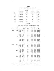
TABLE I. Response Functions for Site I (ltcm s)
Year (n) R(I,I,n) R(I, 2, n) R(I, 3, n) RO, 4, n) R(I, 5, n)
I 184.221 88.0797 107.9536 69.3484 76.6602
2 67.3156 63.1493 64.6223 60.5776 61.6929
3 58.8358 58.0890 58.3932 57.6123 57.8825
4 56.9865 56.7217 56.8383 56.5903 56.6886
5 56.1180 56.0089 56.0605 55.9638 56.0069
6 55.4962 55.4495 55.4729 55.4325 55.4528
7 54.9679 54.9477 54.9581 54.9411 54.9507
8 54.4902 54.4816 54.4859 54.4793 54.4837
9 54.0473 54.0440 54.0454 54.0434 54.0452
10 53.6319 53.6309 53.6308 53.6309 53.6315
II 53.2392 53.2392 53.2385 53.2394 53.2394
12 52.8660 52.8665 52.8655 52.8668 52.8664
J3 52.5100 52.5106 52.5095 52.5109 52.5104
14 52.1691 52.1698 52.1686 52.1701 52.1696
15 51.841& 51.8426 51.8414 51.8428 51.8423
16 51.5269 51.5276 51.5265 51.5279 51.5274
17 51.2231 51.2227 51.2227 51.2241 51.2236
18 50.9296 50.9303 50.9292 50.9306 50.9301
19 50.6455 50.6462 50.6452 50.6465 50.6460
20 50.3701 50.3708 50.3698 50.3710 50.3706
Only response functions for extraction wells are listed.
eight injection wells. The extraction and injection rates are
given in columns 15 through 23. In the second construction
interval, one additional high pressure and one additional low
pressure turbine are added giving a rated total capacity of 27
MW. The plant actually generates 23.3 MW. Two extraction
wells are added but the number of injection wells remains
unchanged. In the third construction interval one high pressure
turbine is added giving a rated total capacity of 29 MW.
Site 4 is developed and the third construction interval
injection well is added at site 8 and 12. No additional wells
are added at site 3; the plant generates 28.9 MW. In the final
construction interval, no additional power plant and well
capacity is added. The actual power generated drops from
28.9 to 23.2 MW. The gradual rise then sudden drop in power
production is due to the single phase flow constraint. For
unrestricted recharge of available water after a 15% loss of
fluid, over 403,000 gal of water at 85°C is reinjected from the
sixth through the tenth time periods. Large injections of
lower temperature fluid could reduce the temperature distribution
throughout the reservoir (even though the reservoir
remains single phase), thus violating the constant temperature
assumption. To determine temperature changes pro-'
duced by the extraction and injection values for the 15%
loss, tests were made using a temperature-pressure single
phase model [Mercer et al., 1975J. It was found that the
maximum temperature changes were less than 2°C. Hence
TABLE 2. Initial Conditions for Power Plant (Exogenous Variables)
the constant temperature assumption is not violated to a
degree to warrant modeling of temperature variation.
CONCLUSIONS
Three assumptions concerning the reservoir model provide
the linear form of the equation offlow (equation (9»: the
reservoir contains only pure water; the reservoir is liquid
dominated; and the spatial distribution of temperature for
the reservoir is known and invarient with time. If any of
these assumptions are invalid for application to a geothermal
reservoir, the flow equation may become coupled with an
additional equation relating . changes in concentration,
changes in phase, or changes in temperature due to withdrawals.
This coupling is generally nonlinear.
If concentrations of dissolved solids are greater than 2%
by weight, the thermodynamic equations «1) and (2» may
require modification such that the viscosity and density
become dependent on concentration. If concentrations are
assumed to be uniform throughout the reservoir, withdrawals
will not induce changes in concentrations and (9) is still a
valid approximation. However, if the concentrations are
nonhomogeneous; withdrawals will induce changes in the
concentrations, and the flow equation is coupled via the
velocity field, to an equation describing the rate of change of
concentrations (for example, see INTERCOMP [1976]).
If fluid in the reservoir undergoes a change from single
Liquid Vapor Liquid Vapor
Pressure, Enthalpy, Enthalpy, Entropy, Entropy,
dynetcm 2 erg/g erg/g erg/g °C erg/g °C
After primary 1.256 x 10 7 (PI) 8.053 x 10 9 2.786 X 1010 2.231 X 10 7 6.512 x W
separator-flasher
Into low pressure 3.495 x 10 6 (P 2 ) 5.818 x 10 9 2.548 X 1010 1.722 X 10 7 6.945 X 10 7
turbine
I nto back compressor 2.026 x 10 5 (P 3 ) 2.514 x 10 9 2.457 X 1010 8.320 X 10 6 7.908 X 10 7
At atmospheric 1.013 x 10 6 (P a ) 4.174 X 10 9 2.506 X 1010 1.303 X 10 7 7.359 X 10 7
Out of dump 3.000 x 10 9
condenser
Efficiencies (mechanical .... electrical): high pressure turbine, 0.85; low pressure turbine, 0.65; back compressor, 0.85.

ewritten as
MADDOCK ET AL.: GEOTHERMAL POWER,
(A5)
where 'TIs is the isentropic efficiency for the turbine (which
has been specified, by assumption). Thus
h/ = hl - 'TI.(hl - hl)
The steam fraction at the outlet is obtained as
T _ h/- hloT
Xs3 - h T _ h T
vo 10
(A6)
(A7)
Compressor. The energy-material balance calculations
for the back pressure compressor are similar to those for the
turbines. As with the turbine calculations the first step is to
determine the steam fraction and the enthalpy of the fluid at
the outlet pressure (atmospheric) for an isoentropic process.
Expressions analogous to (A3) and (A4) are used for this
purpose. To obtain the final enthalpy and steam fraction, the
isoentropic efficiency of the process is used in equation
analogous to (A6) and (A7).
Condenser. The cooling water requirement per gram of
fluid being cooled is given by
h{ - h/
'Ye = C !:t.T
p e
(AS)
where subscripts i and 0 refer to inlet and outlet values of
material being cooled, C p is the heat capacity of the cooling
water, and !:t.Te is the temperature rise allowed for the
cooling wilter.
The intensive electrical work output is determined by
multiplying the intensive mechanical work WTby an efficiency
factor, that is,
Wek = 'TIek . WTk k = 1,2 (A9)
where the k subscript indicates the type of turbine system; k
= 1 for high pressure and k = 2 for low pressure.
The power plant model is run for each of the it.fEPotential.
sites for extraction well development. If WelW and We2W are
the intensive electrical work produced from the high pressure
turbines and low pressure turbines, respectively, for the
jth site, then the electrical power produced iii the power
plant for the ith time period, AMw(I), is
ME
AMw(1) = L (WeIW + W..z(})QEJj, 1)
j=1
(A 10)
where QFfj, I) is the total withdrawal rate from extraction
wells at thejth site in the ith year. Likewise if 'YctW and 'Yd})
are the intensive cooling water requirements for the condenser
on the low pressure turbine and the dump condenser,
respectively, for the jth site, then the rate of cooling water
required for the ith time period, r(i) is
ME
r(i) = L ('YcI(]) + 'Yc2W)QFfj, i)
j=1
(All)
Steam rates entering or exiting the various components of
the power plant are calculated in the same fashion. For
example, if xtw is fraction of steam exiting the primary
separator-flasher system for waters from the jth site, then
the total rate of steam exiting that system in the ith time
period, Ssp(i), is
ME
Ssp(i) = L xtw QFfj, i)
j=l
511
(AI2)
Finally, it should be noted that WekW's, 'Yck(})'S and the
Xk(])'S are independent of the QFfj, i),s, the pressure drops
and the time periods; but they are dependent on the reservoir
temperatures, which remain invariant, and on the operating
temperatures or pressures specified for each component of
the power plant. This is a direct result of assumption 5 in the
power plant model section.
cf>
p(i, t)
k(i)
J.«..i, t)
p(i, t)
g
D(i)
-ql(i, t)
Cv
p,(i)
Cvr
T(i, t)
km(i)
Cv l
TI
b(x)
{3
NOTATION
porosity (dimensionless).
density of water (ml- 3 ).
permeability tensor (12).
viscosity of water (ml- I t- I ).
pressure (ml- 1 C 2 ).
gravitation constant (It- 2 ).
depth (I).
water mass source term (ml- 3 C l ).
specific heat of water (m12 C 2 T- I ).
rock density (ml- 3 ).
specific heat of rock (m12 C 2 T- I ).
temperature (T).
medium thermal conductivity (mlt- 3 T- 1 ).
specific heat of source water (m1 2 C 2 T- 1 ).
temperature of source water (T).
thickness (I).
liquid compressibility (lt 2 m- I ).
REFEItENCES
Bloomster, C. H., GEOCOST: A computer program for geothermal
cost analysis, Rep. BNWL-1888, Battelle Northwest Lab., Richland,
Wash., 1975a.
Bloomster, C. H., Economic analysis of geothermal energy costs,
Rep. BNWL-SA-5596, Battelle Northwest Lab., Richland, Wash.,
I 975b.
Bloomster, C. H., and C. A. Knutsen, The economics of geothermal
electricity generation from hydrothermal resources, Rep. BNWL-
1989; Battelle Northwest Lab., Richland, Wash., 1975.
Faust, C. R., and J. W. Mercer, Geotherinal reservoir simulation, I,
Mathematical models for liquid and vaporcominated hydrothermal
systems, Water Resour. Res., 15(1), 26, 1979.
Grindley, G. W., The geology, structure, and exploitation of the
Wairakei geothermal field, Taupo, New Zealand, N. Z. Geol.
Surv; Bull .• 75, 131 pp., 1965.
Haas, J. L., Jr., Preliminary 'steam tables' for boiling NaCI solutions,
physical properties of the coexisting phases and thermochemical
properties of the H 20 component, U.S. Geol. Surv.
Open File Rep., 75-674. 1975a:
Haas, J. L., Jr., Preliminary 'steam tables' for boiling NaCl solutions,
thermophysical properties of the coexisting phases and
thermochemical properties of the NaCI component, U.S. Geo/.
Surv. Open File Rep .• 75-675, 1975b.
Huber, H., D. H. Bloomster, and R. A. Walter, User manual for
GEOCOST: A computer model for geothermal coast analysis,
Rep. BNWL-1942, Battelle Northwest Lab., Richland, Wash.,
1975.
lritercomp Resource Development and Engineering, Inc., A model
for calculating effects of liquid waste disposal in deep saline
aquifer, in Water Resource Investigations, Doc. 76-61, 253 pp.,
U.S. Geological Survey, U.S. Government Printing Office, Washington,
D. C., June 1976.
Koenig, J. B., Worldwide status of geothermal resources, in Geothermal
Energy, edited by P. Kruger and C. Otte, pp. IS-58,
Stanford University Press, Stanford, Calif., 1973.