"INDUCED POLARIZATION DATA AT ... - University of Utah
"INDUCED POLARIZATION DATA AT ... - University of Utah
"INDUCED POLARIZATION DATA AT ... - University of Utah

You also want an ePaper? Increase the reach of your titles
YUMPU automatically turns print PDFs into web optimized ePapers that Google loves.
GL04031<br />
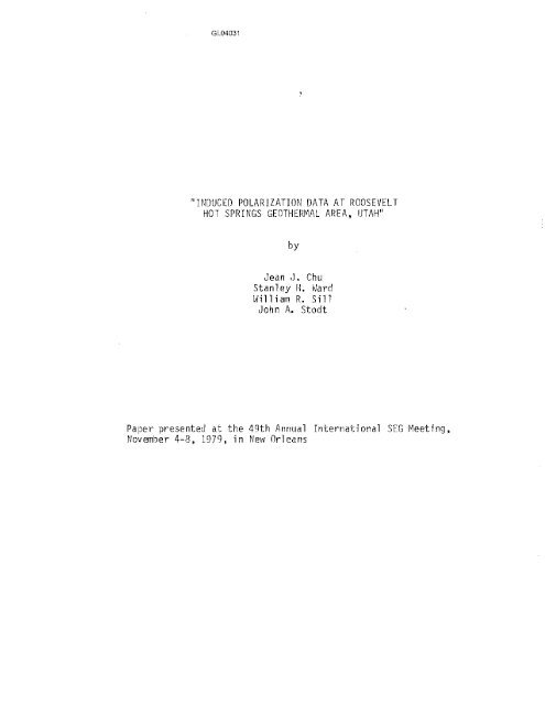
"<strong>INDUCED</strong> <strong>POLARIZ<strong>AT</strong>ION</strong> <strong>D<strong>AT</strong>A</strong> <strong>AT</strong> ROOSEVELT<br />
HOT SPRINGS GEOTHERMAL AREA, UTAW<br />
by<br />
Jean J. Chu<br />
Stanley H. Ward<br />
Wi 11 i am R. S i 11<br />
John A. Stodt<br />
Paper presented at the 49th Annual International SEG Meeting,<br />
November 4-8, 1979, in New Orleans
ABSTRACT<br />
CHU<br />
Both field and laboratory broadband multispectral data have been<br />
gathered in a study <strong>of</strong> IP phenomena at the Roosevelt Hot Springs<br />
geothermal area. The field survey involved two traverses across the<br />
main part <strong>of</strong> the present day hydrothermal system. The laboratory<br />
research gathered data at 25°C, 50°C, and 75°C, on hydrothermally<br />
altered rocks from the hot springs area.<br />
Laboratory data indicate a small IP effect <strong>of</strong> 3 to 23 mr at low<br />
frequencies (0.004 Hz). High frequency (10 3 Hz) IP data ranged from 20<br />
to 100 mr. The IP effect is frequency dependent, and is not affected<br />
markedly by moderate changes in temperature; it is also dependent upon<br />
the quantities <strong>of</strong> pyrite and clay minerals. Pyrite affects the phase<br />
spectrum well above 1 Hz, and its effect is different from that <strong>of</strong><br />
polarizable clays.<br />
The field data at the higher frequencies show both positive and<br />
negative phase values, which can be explained by electromagnetic<br />
coupling. Extrapolated phase data reveal a small anomalous region <strong>of</strong> 20<br />
to 34 mr along one <strong>of</strong> the pr<strong>of</strong>iles; the majority <strong>of</strong> the data ranged from<br />
7 to 15 mr.<br />
The laboratory and field data indicate only a small IP effect over<br />
the hydrothermal system; it could be considered as background and hence<br />
<strong>of</strong> no consequence. There seems to be no large scale delineation <strong>of</strong> the<br />
geothermal field.
INTRODUCTION<br />
CHU<br />
The purpose <strong>of</strong> this study was to investigate the usefulness <strong>of</strong><br />
conducting an induced polarization (IP) survey in a geothermal<br />
environment <strong>of</strong> the high temperature convective hydrothermal type. Can<br />
one utilize the polarization characteristics <strong>of</strong> clays and pyrite to<br />
distinguish zones <strong>of</strong> low resistivity due to hydrothermal alteration from<br />
those due solely to the presence <strong>of</strong> hot brines?<br />
Risk (1975), in a resistivity survey <strong>of</strong> the Broadlands geothermal<br />
field, New Zealand, briefly mentioned detection <strong>of</strong> an IP anomaly,<br />
suggesting its probable cause as disseminated sulfide minerals. Induced<br />
polarization surveys over geothermal systems have been conducted by<br />
Zohdyet al (1973), and Ross (1979). The former employed a pole-dipole<br />
array, using 0.1 Hz and 1.0 Hz, while the latter used the dipole-dipole<br />
array with measurements taken in the time domain. In both cases, IP<br />
anomalies were recorded: Zohdy et al (1973), working in the Mud Volcano<br />
area <strong>of</strong> Yellowstone' National Park, cited the relatively high<br />
concentrations <strong>of</strong> pyrite as the probable cause <strong>of</strong> the anomalies; Ross<br />
(1979) stated that the polarization data gathered in the Cove Fort -<br />
Sulphurdale thermal area, <strong>Utah</strong>, were too limited to speculate on the net<br />
polarization characteristics due to pyrite, clay and zeolite<br />
mineralization. These surveys indicated the need for documented study<br />
<strong>of</strong> IP phenomena in geothermal areas. It was to fulfill this need that<br />
broadband multispectral data were gathered both in the field and in the
laboratory during the years <strong>of</strong> 1978 and 1979.<br />
CHU<br />
The geothermal system chosen for this study was the Roosevelt Hot<br />
Springs Known Geothermal Resource Area (KGRA) (Figure 1). This area<br />
contains a structurally controlled, hot-water dominated system in<br />
plutonic and metamorphic rock (Nielson et al, 1978). Oetailed<br />
geological, geochemical and geophysical work has led to the development<br />
<strong>of</strong> a complete case study <strong>of</strong> the area (Ward et al, 1978). Extensive<br />
electrical data have been gathered involving 100 m, 300 m, and 1 km<br />
dipole-dipole resistivity, Schlumberger resistivity, electromagnetic,<br />
and magnetotelluric soundings. In addition, controlled source audio<br />
magnetotelluric, bipole-dipole resistivity, telluric ratio, and self<br />
potential surveys have been conducted. The geology <strong>of</strong> the area is<br />
summarized by Ward et al (1978); detailed geology is given by Nielson et<br />
al (1978). Research in this region continues to the present.<br />
Induced polarization in the frequency domain is a phenomenon<br />
whereby resistivity changes as a function <strong>of</strong> frequency. This effect is<br />
produced by the presence <strong>of</strong> clays, zeolites, conductive oxides and<br />
conductive sulfides. In the Roosevelt Hot Springs thermal area,<br />
extensive hydrothermal alteration has produced clays, pyrite and<br />
marcasite (Parry et al, 1978; Ballantyne and Parry, 1978). A monitoring<br />
<strong>of</strong> the IP phenomena due to these alteration minerals might allow us to<br />
map the zones <strong>of</strong> alteration. Our study was conducted to assess this<br />
possibility.<br />
We present our results in three sections. Laboratory data are<br />
given first, with schematic explanations <strong>of</strong> the possible reasons behind<br />
the IP behavior <strong>of</strong> hydrothermally altered rocks. Data from the field<br />
survey follow, and we discuss the methods available to remove inductive
FIG. 2' Location map <strong>of</strong> Roosevelt Hot Springs KGRA. Base line, heat flow<br />
(mW/m ) and apparent resistivity (n-m) contours from Ward et al (1978). IP<br />
traverses with dipole-dipole array shown as Lines 1 and 2. Productive wells<br />
shown by solid dots, IIdry wells ll by open circles. Cores for laboratory<br />
research taken from three shallow alteration holes shown by circles with<br />
crosses. Hachured re[ion is bedrock exposure <strong>of</strong> Mineral Mountains; white area<br />
is quaternary alluvium; black areas are quaternary sinter deposits and altered<br />
rock. The area <strong>of</strong> highest heat flow is shaded. The Opal Mound Fault is<br />
shown.<br />
CHU
electromagnetic (EM) coupling from the field measurements. In the final<br />
CHU<br />
section, we summarize and integrate the essentials from the laboratory<br />
and field data, and draw conclusions.
Data Acquisition<br />
LABOR<strong>AT</strong>ORY RESEARCH<br />
CHU<br />
Parry et al (1980) analyzed the subsurface alteration in three<br />
shallow diamond drill holes (maximum depth: 70m) located near the Opal<br />
Mound Fault (Figure 1). On the basis <strong>of</strong> their data, core samples were<br />
selected covering the spectrum <strong>of</strong> low to high clay and pyrite content.<br />
Sample preparation. - The cores were 4.7cm in diameter with lengths<br />
varying from 4.8cm to 7.2cm. Most <strong>of</strong> the altered samples were friable,<br />
consequently, each core sample was enclosed in epoxy. The epoxy itself<br />
showed no significant IP effects.<br />
Expansion and cracking <strong>of</strong> the sample holders were avoided by<br />
soaking those rocks with montmorillonite content greater than 10 weight<br />
percent in distilled water prior to complete enclosure in the epoxy.<br />
Holes were drilled into the ends <strong>of</strong> the enclosed samples. They were<br />
then vacuum saturated with 0.1 N NaCl solution, which is approximately<br />
the same concentration as the brine encountered in the Roosevelt Hot<br />
Spri ngs thermal area (Parry et al, 1978).<br />
Apparatus and experimental procedure. - A phase-sensitive receiver<br />
(ZERO, GDP-12/2G) was employed as both a digital voltmeter and a signal<br />
generator. A chart recorder monitored any erratic or drifting behavior<br />
<strong>of</strong> the experimental apparatus. To maintain constant temperature, the
CHU<br />
pore solution. This value is thought to reflect the contribution <strong>of</strong><br />
clays to the IP effect. Qv can be determined independently from the<br />
ratio <strong>of</strong> cation exchange capacity <strong>of</strong> the core sample (meq) to the pore<br />
volume <strong>of</strong> the sample (ml). The cation exchange capacity, CEC, in meq<br />
per 100gm <strong>of</strong> the rock sample, was measured by atomic absorption<br />
spectrometry. A summary <strong>of</strong> the measurements is given in Table 1.<br />
Both Qv and porosity depend upon the volume <strong>of</strong> interconnected pore<br />
passages within the rock. For non-expanding core samples, the pore<br />
volume was taken to be the volume <strong>of</strong> water absorbed by the rock after<br />
the two to three month soaking period. For samples which expanded [(c)<br />
and (f) <strong>of</strong> Table 1J, the pore volume was assumed to be the difference<br />
between the volume <strong>of</strong> water absorbed and the change in volume <strong>of</strong> the<br />
core sample. This latter procedure may have resulted in inflated QV<br />
values; but if the former procedure had been followed, the QV values for<br />
the expanded samples (c) and (f) would have been 1.34 equiv/l and 2.22<br />
equiv/l respectively, which are still larger than the Qv values for the<br />
non-expanded samples.<br />
The porosity (effective porosity) was determined from the ratio <strong>of</strong><br />
the pore volume <strong>of</strong> the sample to the volume <strong>of</strong> the rock when wet.<br />
Data Interpretation<br />
Ten samples were prepared. Two <strong>of</strong> the samples were slightly<br />
hydrothermally altered, while another two were inadequately<br />
encapsulated. The remaining six samples were highly altered, and the<br />
data for these are shown in Table 1 and Figures 2a-2f.<br />
Effects <strong>of</strong> temperature. - The resistivity <strong>of</strong> the altered rocks is
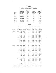
TABLE 1. Parameter values <strong>of</strong> effective porosity, cation exchange capacity<br />
(CEC), clay (Qv) and pyrite content, for six core samples identified by drill<br />
hole and depth <strong>of</strong> recovery. Labels a-f relate samples to spectra shown in<br />
Figures 2a-2f. Range in IP effect taken from data at 25°C. Resistivity<br />
obtained at room temperature using 1/256Hz.<br />
CHU
Sampl e Resistivity IP effect<br />
(n-m) (mr)<br />
(a) [76-1J 11.5 7-20<br />
30.8m<br />
(b) 1A 5.2 12-37<br />
37.5m<br />
(c) 1A 3.8 12-25<br />
49.7m<br />
(d) lA 6.6 9-92<br />
58.5m<br />
( e) lA 7.1 11-100<br />
61.3m<br />
( f) lA 3.4 7-23<br />
51.2m<br />
Poros i ty CEC<br />
(meq/100 gm)<br />
0.33 4<br />
0.30 19<br />
0.20 35<br />
0.36 8<br />
0.28 15<br />
0.15 52<br />
Qv<br />
(equiv/1)<br />
0.22<br />
1.23<br />
3.2<br />
0.46<br />
1. 22<br />
6.2<br />
Pyrite<br />
(wt.%)<br />
0.2<br />
1.0<br />
2.4<br />
4.3<br />
8.6<br />
9.1<br />
Cf/U<br />
Table- I
FIGS. 2a-2f. Laboratory data arranged in increasing pyrite content, for<br />
frequency range 1/256 Hz to 1024 Hz. Electrolyte is 0.1 N NaCl. For<br />
resistivity plot, lower 25°C curve taken after sample cooled from 75°C; data<br />
for rocks wnere 25°C curves differed by less than 0.3 Q-m have been<br />
combined. Sample (c) heated to 50°C only. For phase plot, double set <strong>of</strong> data<br />
at 25°C averaged (solid dots); vertical lines and open circles represent 50°C<br />
and 75°C range in values. Horizontal bar graphs represent polarizable clay<br />
(Qv) and pyrite content.<br />
CHU
determined by rock porosity, the electrical properties <strong>of</strong> the pore fluid<br />
and the clay and pyrite content. In this study, the resistivity <strong>of</strong> the<br />
electrolyte is set and monitored, leaving porosity, and clay and pyrite<br />
content as variable factors. The influence <strong>of</strong> porosity alone is<br />
expressed by Archie's Law, while that including the contribution <strong>of</strong> clay<br />
CHU<br />
can be found in an expression developed by Waxman and Smits (1968).<br />
Temperature dependent fomls <strong>of</strong> these two expressions can be obtained by<br />
referring to Keller and Frischknecht (1966, p. 31), and Waxman and<br />
Thomas (1974).<br />
We found that core samples with high Qv values [(c) and (f) <strong>of</strong><br />
Table IJ behaved according to the Waxman-Smits model, while those with<br />
lower Qv values [(a), (d), and (e) <strong>of</strong> Table IJ had resistivities which<br />
followed Archie's Law. By varying the porosity exponent, we can fit the<br />
data for sample (b) using either Archie's Law or the Waxman-Smits model.<br />
The effect <strong>of</strong> temperature on resistivity and phase spectra is shown<br />
in Figures 2a-2f. Rock resistivities change as a function <strong>of</strong><br />
temperature according to the above two models. The phase spectra show<br />
small changes in character as temperature is increased. At the highest<br />
frequencies, the phase values drop by 10 to as much as 22 milliradians<br />
in Figures 2a, 2b, 2d, and 2e. For eight <strong>of</strong> the ten samples measured,<br />
phase values at the lower frequencies did not change by more than 4mr as<br />
the temperature was increased; for two samples, a phase change <strong>of</strong> 8mr<br />
occurred from 25°C to 75°C.<br />
Effects <strong>of</strong> Frequency. - Figures 2a-2f illustrate the frequency<br />
dependence <strong>of</strong> the hydrothermally altered core samples. As frequency<br />
increased, the greatest change in the phase curves occurs in samples (d)
and (e). Both samples have comparatively high pyrite content and<br />
relatively low Qv values. The behavior <strong>of</strong> their respective resistivity<br />
curves follow the observations made by DeWitt (1978) and Wong (1979); as<br />
CHU<br />
the metallic content in a rock increases, the IP effect increases.<br />
We now examine the phase spectra behavior <strong>of</strong> the laboratory data at<br />
and below 32Hz, i.e. the frequency range used in the field survey. For<br />
the samples (c) and (f), which have very high QV values, the phase<br />
spectra are approximately independent <strong>of</strong> frequency. Samples (b), (d),<br />
and (e) exhibit a definite frequency dependence in the phase curves,<br />
even to the lowest frequency. Sample (a), which is low in both pyrite<br />
and Qv value, has a flat phase spectrum. However, the phase spectrum <strong>of</strong><br />
another sample (not shown here) with similar low pyrite and clay content<br />
(room temperature resistivity: 50n-m) shows a smooth drop in phase<br />
values from 12mr to 3mr over the frequency range <strong>of</strong> 114Hz to 1/256 Hz.<br />
For yet another sample (also not shown) the phase value changes from<br />
14mr at 1Hz, to 11mr at 1116Hz, and finally to 17mr at 1/256Hz. Such<br />
data were reproducible, and well above the measurement noise level for<br />
these samples. Thus, hydrothermally altered rocks can exhibit IP<br />
effects that are frequency dependent at low frequencies.<br />
In closing, for the entire suite <strong>of</strong> ten samples, the phase values<br />
recorded at the lowest frequency varied from 3mr to 23mr. At the<br />
highest frequency <strong>of</strong> 1024Hz, phase values ranged from 20 to 100mr.<br />
The effect <strong>of</strong> clays and pyrite on phase spectra. - Previous<br />
laboratory measurements (Tripp, pers. com.) on altered material have<br />
shown low frequency «1Hz) phase anomalies, which have been attributed<br />
to the effect <strong>of</strong> pyrite; higher frequency (>lHz) polarization is thought
CHU<br />
to be due to the presence <strong>of</strong> clays and fine grained material (DeWitt,<br />
1978). We can assess the validity <strong>of</strong> this hypothesis by an examination<br />
<strong>of</strong> the laboratory phase data (solid dots) shown in Figure 2a-2f. We<br />
first examine the phase spectra with respect to pyrite content: spectra<br />
(a) through (f) have been arranged according to increasing pyrite<br />
content, as shown by the bar graphs. We note an abrupt change in<br />
spectrum character when the pyrite content is about 3% (c and d).<br />
Another change occurs between (e) and (f). With the exception <strong>of</strong><br />
samples (c) and (f), the maximum measured phase increases with<br />
increasing pyrite content. In contrast, examination <strong>of</strong> the spectra in<br />
terms <strong>of</strong> increasing Qv values (bar graphs) shows no obvious trends.<br />
The various effects <strong>of</strong> clay and pyrite can be explained by<br />
consideration <strong>of</strong> the IP models proposed by DeWitt (1978) and Wong<br />
(1979). Both models give similar results but the parameters <strong>of</strong> DeWitt's<br />
model are more useful in the discussion that follows.<br />
The model <strong>of</strong> DeWitt (1978) predicts that the maximum phase angle<br />
occurs at the frequency<br />
and that the maximum phase at this frequency is<br />
where<br />
v = volume fraction <strong>of</strong> polarizable spheres,<br />
a = radius <strong>of</strong> polarizable spheres,<br />
(1)
PI = background (rock) resistivity,<br />
A = magnitude <strong>of</strong> the surface impedance at W = 1, and<br />
C = frequency dependence <strong>of</strong> the surface impedance<br />
(C = .5 for diffusion and C = 1.0 for charge separation).<br />
The model predicts that the frequency at which the peak <strong>of</strong> the phase<br />
dispersion occurs depends mainly on the background resistivity (PI) and<br />
the grain size (a), since the magnitude (A) and the frequency dependence<br />
(C) <strong>of</strong> the surface impedance are relatively constant for a given<br />
polarizable material. The maximum phase, on the other hand, depends<br />
mainly on the volume fraction <strong>of</strong> the polarizable material present.<br />
These models have been developed specifically for conducting spheres but<br />
they might be expected to indicate the general trends for clay<br />
polarization as well. The grain size <strong>of</strong> the pyrite particles was<br />
determined by optical examination in reflected light <strong>of</strong> polished<br />
sections taken from drill holes 76-1 and 1A (Figure 1). The average<br />
size was found to be 0.06mm with a standard deviation <strong>of</strong> .02mm. The<br />
size <strong>of</strong> clay minerals tends to be less than about 211 (Grim, 1968). If<br />
we assume that the above models work not only for conductive minerals<br />
but for any polarizable material, we can expect on the basis <strong>of</strong> grain<br />
size alone that the maximum phase for clays will appear at a higher<br />
frequency than that for pyrite.<br />
Putting the mean grain size <strong>of</strong> the pyrite into equation 1 and using<br />
the sample resistivities and A = 2nm 2 , C = 0.65, the frequency <strong>of</strong><br />
maximum phase is typically found to be above 1KHz. Thus in the sampl e<br />
meas urements, the meas ured phases are probably due to contri but ions from<br />
clay and pyrite, both <strong>of</strong> which have dispersion peaks above the frequency<br />
CHU
window <strong>of</strong> the laboratory measurements.<br />
CHU<br />
There is evidence to justify placing the phase spectrum peak <strong>of</strong> the<br />
clay and pyrite grain size groups above 1024Hz. Hall<strong>of</strong> et al (1979), in<br />
describing massive sulfide mineralization, indicated peaks well above<br />
3Hz. DeWitt (1978) recorded measurements on two core samples from the<br />
Tyrone prophyry copper deposit near Silver City, New Mexico, and<br />
compared his data with some in situ IP measurements made at the same<br />
deposit by Pelton et al (1978). He found that the dispersion related to<br />
the sulfide response was reasonably separated from a higher frequency<br />
dispersion whose peak was above 10 5 Hz, which he attributed to membrane<br />
polarization <strong>of</strong> alteration minerals. Finally, Tripp (1977), gathered<br />
data up to 10 5 Hz on core samples from the shallow alteration holes lA<br />
and IB (Figure 1). The spectra showed a steady upward trend in phase<br />
values, similar to the phase curves <strong>of</strong> Figures 2a-2f. Most <strong>of</strong> his IP<br />
data indicated peaks well above 105Hz. However, one <strong>of</strong> his samples<br />
showed a phase dispersion peak at approximately 5xl03Hz (Pelton, 1977,<br />
p. 113), which could be attributed to possible pyrite mineralization<br />
(Tripp, per. com.).<br />
A possible explanation for the changes in the phase spectra between<br />
Figures 2b and 2e is shown in Figure 3. Since the polarizable clay<br />
content, expressed as Qv, is essentially the same for these samples, the<br />
clay dispersion as shown in Figure 3 is the same for both samples.<br />
Increasing the pyrite content causes an increase in the phase curve as<br />
shown in the sketch.<br />
The change in spectra between samples (e) and (f) (Figures 2e and<br />
2f) might be the result <strong>of</strong> the effects shown in Figure 4. In thi s case
FIG. 3. A schematic explanation <strong>of</strong> phase spectra in Figures 2b and 2e, based<br />
on conclusions from DeWitt (1978) and Wong (1979). Bottom curves represent<br />
spectral dispersions associated with clay and pyrite grain size groups; clay<br />
dispersion is fixed. Summation <strong>of</strong> respective dispersion curves shown in upper<br />
diagram; sketch <strong>of</strong> laboratory data drawn with solid lines.<br />
CHU
FIG. 4. A schematic explanation <strong>of</strong> phase spectra shown in Figures 2e, 2f,<br />
based on studies by DeWitt (1978) and Wong (1979). Bottom curves represent<br />
spectral dispersions associated with clay and pyrite grain size groups.<br />
Summation <strong>of</strong> respective dispersion curves shown in upper diagram; sketch <strong>of</strong><br />
laboratory data drawn with solid lines.<br />
CHU
CHU<br />
the pyrite contents are about the same but the clay content (Qv) <strong>of</strong><br />
sample (f) is larger. The increased clay content has lowered the<br />
background resistivity <strong>of</strong> sample (f) and according to equation (1) the<br />
pyrite and clay dispersions, labelled "PYRITE f" and "CLAY f"<br />
respectively, have been moved to higher frequencies. Summing up the<br />
effects as in the top <strong>of</strong> the figure gives a sketch <strong>of</strong> the observed data.<br />
The lowering <strong>of</strong> the background resistivity as temperature increases<br />
might also be expected to shift the phase dispersions <strong>of</strong> our samples.<br />
As noted previously, for samples (a), (b), (d), and (e), there is a<br />
noticeable drop <strong>of</strong> as much as 22mr in the magnitude <strong>of</strong> the phase values<br />
at the highest frequencies. This may be due to the fact that as<br />
temperature increases, the resistivity <strong>of</strong> the rock sample decreases; the<br />
phase spectrum <strong>of</strong> the rock will shift slightly up frequency, as shown<br />
schemat icall yin Figure 5. In the frequency range <strong>of</strong> the 1 ab data, thi s<br />
shift is perceived as a drop in phase values for the positive slope <strong>of</strong><br />
the phase spectrum, and an increase in phase values for the negative<br />
slope <strong>of</strong> the spectrum (see phase spectra in Figures 2b and 2d). Figure<br />
5 also shows that one may be able to gain more information on low<br />
frequency phase behavior by increasing temperature. An exception to the<br />
above sample (f) <strong>of</strong> Figure 2f, which behaves in an opposite manner at<br />
the higher frequencies: the phase rises by about 20mr at 75°C.
FIG. 5. Schematic explanation <strong>of</strong> temperature effect on phase spectrum for<br />
sample (b) <strong>of</strong> Figure 2b. Heavy lines denote frequency range <strong>of</strong> lab data. The<br />
drop in resistivity as temperature rises, shown by the resistivity plot,<br />
causes the phase spectrum to shift to a higher frequency; thus one may be able<br />
to gain more information on the phase behavior at low frequencies by<br />
increasing temperature.<br />
CHU
- E<br />
q<br />
- r<br />
t-<br />
><br />
C/)<br />
lJJ<br />
0::<br />
- lJJ<br />
-"-<br />
E<br />
en<br />
Data Acquisition<br />
FIELD SURVEY<br />
CHU<br />
During the summer <strong>of</strong> 1978, 15 line-km <strong>of</strong> multi-frequency IP data<br />
were obtained across the Roosevelt Hot Springs geothermal system, along<br />
the two pr<strong>of</strong>iles shown in Figure 1. Line 1 crosses the southern half <strong>of</strong><br />
the geothermal system while Line 2 crosses the northern portion. The<br />
zone <strong>of</strong> maximum hydrothermal alteration (Parry et al, 1980) is situated<br />
between Lines 1 and 2. However, permit restrictions limited the<br />
traverses to roadways only, and hence the location and configuration <strong>of</strong><br />
the pr<strong>of</strong>ile lines. The western ends <strong>of</strong> Lines 1 and 2 correspond to 2200<br />
Nand 5950 N, respectively, <strong>of</strong> the dipole-dipole resistivity survey grid<br />
established by Ward and Sill (1976); the base line <strong>of</strong> this grid is also<br />
shown in Figure 1.<br />
Drill hole data revealed that polarizable clays were primarily<br />
confined to the upper portion <strong>of</strong> the holes (Ballantyne and Parry, 1978:<br />
Rohrs and Parry, 1978; Ballantyne, 1978). The depth <strong>of</strong> K-feldspar<br />
stability was estimated at 400m (Ward and Sill, 1976). To resolve zones<br />
<strong>of</strong> possible alteration, we used the collinear dipole-dipole array, with<br />
dipole lengths <strong>of</strong> 100m and 300m and maximum n spacings <strong>of</strong> 4 and 6,<br />
respect ivel y.<br />
The equipment used in the survey included the ZERO phase-sensitive<br />
receiver (GDP-12/2G), a Geotronics FT20A transmitter and a motor
FIG. 9. 20 resistivity model (bottom) for Line 2. Contoured apparent<br />
resistivity data (top) obtained at 1/256 Hz with 300 m dipoles. Contour and<br />
model pattern codes same as in Figure 8. Resistivity <strong>of</strong> model blocks in Qm.<br />
Based on Figure 10, faults exposed at the surface are indicated by IIfll;<br />
inferred faults shown with II ?".<br />
CHU
CHU<br />
modeled resistivity contrasts between stations 3 East and 18 West in<br />
Figure 8 coincide with the faults crossing Line 1 in Figure 10. The<br />
Opal Mound Fault is located at station 12 West along Line 1 (Figures 1,<br />
10, and 8).<br />
Soil sample analyses (Capuano and Bamford, 1978; Bamford et al,<br />
1980) indicate a possible fault passing through the area near well 72-16<br />
and station 6 West <strong>of</strong> Line 1 (Figure 10). The modeled resistivity data<br />
(Figure 8) also suggest a fault; the 300m dipole data show a contrast <strong>of</strong><br />
12 to 50n-m at station 6 West.<br />
Figure 9 shows the resistivity model for Line 2. The majority <strong>of</strong><br />
the computed resistivities were within 10% <strong>of</strong> the observed<br />
resistivities. The surface locations <strong>of</strong> the modeled resistivity<br />
contrasts marked IIfll correspond to faults crossi ng Line 2 in Figure<br />
10. Dashed lines in Figure 10 are inferred faults and correspond to the<br />
resistivity contrasts marked by II?II in Figure 9.<br />
Figures 8 and 9 show high resistivities on the eastern parts <strong>of</strong> the<br />
survey lines near the Mineral Mountains, with a transition to lower<br />
resistivities toward the west. The zones <strong>of</strong> low resistivity modeled in<br />
both lines over the geothermal system extend westward beneath more<br />
resistive material. A likely geological explanation for this is that<br />
brine is 1 eaki ng from the co nvect i ve hydrothermal system westward<br />
beneath the valley sediments. At station 39 <strong>of</strong> Line 2 in Figure g, the<br />
resistive over conductive regime changes to a conductive over resistive<br />
regime. We assessed the character and magnitude <strong>of</strong> phase shifts due to<br />
coupling over these two regimes by calculating the one-dimensional EM<br />
coupling for the dipole-dipole array (Hohmann, 1973). Figure 11 shows
FIG. 10. Fault pattern in survey area based on geological evidence (Nielson et<br />
al,1979). Solid lines indicate faults verified in the field; dashed lines<br />
indicate inferred faults. Relative fault movement marked by U, D. Shaded<br />
area is Mineral Mountains; white area is alluvium; black areas are altered<br />
rocks and sinter deposits. Producing wells shown by solid dots, IIdry wells ll<br />
by open circles, shallow alteration holes by circles with crosses.<br />
CHU
FIG. 11. 10 electromagnetic coupling for two different earth models shown for<br />
dipole-dipole array n spacings <strong>of</strong> 1, 3, and 5. Solid lines are for resistive<br />
over conductive model; dashed lines are for conductive over resistive model.<br />
Depth to interface = 180 m.<br />
CHU
-500<br />
-400<br />
-300<br />
-200<br />
!o- -100<br />
E<br />
.........<br />
w<br />
if)<br />
the coupling calculations. Negative phase values are obtained above 4Hz<br />
for n spacings greater than 1 for the resistive over conductive model.<br />
In contrast, all coupling phase values are positive for the conductive<br />
over resistive model, for the range <strong>of</strong> frequencies and n spacings used<br />
in the field measurements. Comparing these coupling calculations with<br />
the phase pseudosections from Line 1 in Figures 7a-7c, we see that the<br />
field phase data on either side <strong>of</strong> the modeled contact at 39 West agree<br />
in every aspect with the behavior <strong>of</strong> the coupling curves in Figure 11.<br />
Away from the contact, the magnitude <strong>of</strong> the coupling indicated by the<br />
theoretical curves is in good agreement with the observed data at each<br />
CHU<br />
frequency. The good agreement <strong>of</strong> the theoretical coupling and the<br />
observed phase data strengthens the resistivity interpretation on the<br />
western portion <strong>of</strong> Line 2.<br />
Interpretation <strong>of</strong> the IP responses in our phase data from the<br />
Roosevelt Hot Springs thermal area is hindered by telluric noise below<br />
1116Hz. If we avoid telluric noise by utilizing the measurements<br />
obtained at 1116Hz and above, then EM coupling must be removed from the<br />
field data. Techniques to remove EM coupling from field data were not<br />
published until 1974, when Hall<strong>of</strong> proposed a method based on "phase<br />
extrapolation ll<br />
• Since then, two other methods have been suggested, one<br />
which is proprietary (Wynn and Zonge, 1975, 1977), and one which<br />
involves inversion to Cole-Cole models (Pelton et al, 1978). Coupling<br />
removal was attempted using phase extrapolation.<br />
Phase extrapolation. - Hall<strong>of</strong> (1974) proposed fitting phase data, taken<br />
between O.05Hz and 1.25Hz, with a linear or quadratic function.<br />
Extrapolating this function to zero frequency leaves the constant term
FIG. 12. Pseudosections resulting from extrapolation <strong>of</strong> 1Hz, 114Hz, and<br />
1116Hz phase data from Lines 1 and 2. Phase values for Line 1, a = 100 m, fit<br />
into the bottom pseudosection as shown. Dotted contours <strong>of</strong> the top<br />
pseudosection outline areas with negative phase values.<br />
CHU
the model <strong>of</strong> Figure 8.<br />
CHU<br />
A comparison <strong>of</strong> the phase extrapolated data shows some general<br />
similarities to the original data at 1116Hz, although the extrapolated<br />
phases are somewhat smaller. This probably indicates that at this<br />
frequency the EM coupling is less than the true IP effects.<br />
The phase extrapolation technique gives an estimate <strong>of</strong> the minimum<br />
IP response in the frequency band <strong>of</strong> the quadratic fit. Unfortunately,<br />
host rocks surrounding the geothermal area also exhibit approximately<br />
the same magnitude <strong>of</strong> polarization, if the phase extrapolation is<br />
correct. Hence, thi s particul ar geothennal system is not well<br />
delineated by its IP response between 1116Hz and 1Hz.<br />
Changes in background resistivity, percentages <strong>of</strong> polarizable<br />
materials, grain size, or range <strong>of</strong> grain sizes can each produce changes<br />
in the frequency dependence <strong>of</strong> the IP effect. It is possible that<br />
hydrothermal alteration could produce changes in these parameters which<br />
would cause systematic variations in the frequency dependence <strong>of</strong> the IP<br />
response and thus delineate the geothermal area. However, more<br />
sophisticated coupling removal must be effected if the frequency<br />
dependence <strong>of</strong> the IP response in the data is to be examined.
SUMMARY AND CONCLUSIONS<br />
CHU<br />
The laboratory research on the contribution <strong>of</strong> pyrite or marcasite<br />
and clays to the IP effect has resulted in a number <strong>of</strong> empirical<br />
findings:<br />
(i) our hydrothermally altered rock samples do exhibit IP<br />
behavior: at 1/256 Hz, the IP effect is small, from 3 to 23<br />
mr; at 1024 Hz, IP phase values ranged from 20 to 100 mr,<br />
(ii) the IP effect is frequency dependent, even to the lowest<br />
frequencies,<br />
(iii) the resistivity <strong>of</strong> our samples is affected by temperature<br />
and the presence <strong>of</strong> clays; the resistive behavior fits<br />
either Archie's Law or the Waxman-Smits model, depending<br />
upon the clay content,<br />
(iv) the IP effect is not affected markedly by moderate changes<br />
in temperature for the frequency range 1/256 Hz to 1024 Hz,<br />
and<br />
(v) the IP behavior is affected by the presence <strong>of</strong> pyrite, and<br />
<strong>of</strong> clay minerals, the effect <strong>of</strong> pyrite appearing to differ<br />
from that <strong>of</strong> polarizable clay: for the frequency range <strong>of</strong><br />
1/4 Hz to 1024 Hz, pyrite tended to increase the phase<br />
values, while clay tended to decrease the phase values.<br />
If we assume that the IP behavior <strong>of</strong> the rock core sample is<br />
determined solely by the presence <strong>of</strong> polarizable clay and/or pyrite, and
CHU<br />
that the principles illustrated in Figure 3, discovered through the<br />
study <strong>of</strong> synthetic ore samples, hold for any polarizable particle, then<br />
we can add these inferences:<br />
(vi) pyrite affects the phase spectrum well above 1 Hz; the peaks<br />
<strong>of</strong> the phase dispersions associated with pyrite and clay are<br />
above 10 3 Hz,<br />
(vii) the maximum value <strong>of</strong> the phase dispersions associated with<br />
pyrite is at lower frequency than that <strong>of</strong> clay; this is due<br />
mainly to the difference in grain size between the mineral<br />
groups,<br />
(viii) the dispersions <strong>of</strong> clay and pyrite superimpose to explain<br />
the IP effect, and<br />
(ix) the manner in which the dispersions <strong>of</strong> clay and pyrite<br />
contribute to the final phase spectrum <strong>of</strong> the core sample<br />
depends upon the relative positions <strong>of</strong> these two dispersion<br />
curves along the frequency axis, as well as the shape and<br />
magnitude <strong>of</strong> each <strong>of</strong> the dispersion curves; all <strong>of</strong> these<br />
factors are a function <strong>of</strong> several parameters, including the<br />
resistivity <strong>of</strong> the rock, the amount <strong>of</strong> polarizable material<br />
present, and the grain sizes <strong>of</strong> the particles causing the IP<br />
effect.<br />
On the basis <strong>of</strong> these hypotheses, we suggest that our uncoupled<br />
field data are low frequency asymptotes <strong>of</strong> many superposed spectral<br />
dispersions whose main peaks are well above the range <strong>of</strong> frequencies<br />
used in the field.<br />
In conclusion, we note that there is good agreement between the<br />
phase extrapolated field data and the laboratory results. The IP
esponse <strong>of</strong> this hot-water dominated system is generally small, in the<br />
range <strong>of</strong> 7 to 15 mr. The field and laboratory data also indicate that<br />
IP responses <strong>of</strong> from 20 to 34 mr are possible, though infrequent. There<br />
is no large scale delineation <strong>of</strong> the geothermal field. However, it is<br />
important to note that the zone <strong>of</strong> maximum alteration was not sampled by<br />
the two IP traverses documented here.<br />
CHU
ACKNOWLEDGEMENTS<br />
CHU<br />
This research was funded by the Department <strong>of</strong> Energy, Division <strong>of</strong><br />
Geothermal Energy, Contract DE-AC03-79ET27002. Thanks are due to Dr.<br />
W. T. Parry, for his aid in assessing the CEC values by atomic<br />
absorption spectrometry.
REFERENCES<br />
CHU<br />
Ballantyne, G. H., 1978, Hydrothermal alteration at the Roosevelt Hot<br />
Springs thermal area, <strong>Utah</strong>: characterization <strong>of</strong> rock types and<br />
alteration in Getty Oil Company well <strong>Utah</strong> State 52-21: Topical<br />
rep., v. 78-1701.a.l.1.4, DOE/DGE contract EG-78-C-07-1701, Univ.<br />
<strong>of</strong> Ut a h, 24 p.<br />
Ballantyne, J. M., and Parry, W. T., 1978, Hydrothermal alteration at<br />
the Roosevelt Hot Springs thermal area, <strong>Utah</strong>: petrographic<br />
characterization <strong>of</strong> the alteration to 2 kilometers depth: Tech.<br />
rep., v. 78-1701-a.l.1, DOE/DGE contract EG-78-C-07-1701, Univ. <strong>of</strong><br />
<strong>Utah</strong>, 26 p.<br />
Bamford, R. W., Christensen, O. D., and Capuano, R. M., 1980, Multielement<br />
geochemistry <strong>of</strong> solid materials in geothermal systems and<br />
its applications, Part 1: The hot-water system at the Roosevelt<br />
Hot Springs KGRA, <strong>Utah</strong>: Univ. <strong>Utah</strong> Research Inst., Earth Science<br />
Laboratory, report no. 30, DOE/DGE Contract no. DE-AC03-79ET-<br />
27002, 168 p.<br />
Campbell, R. E., 1977, Geophysical drill hole casing anomalies, in<br />
Workshop on Mining Geophysics: S. H. Ward, ed., <strong>University</strong> <strong>of</strong><br />
<strong>Utah</strong>, Dept.<strong>of</strong> Geol. and Geoph.<br />
Capuano, R. M., and Bamford, R. W., 1978, Initial investigation <strong>of</strong><br />
soil mercury geochemistry as an aid to drill site selection in<br />
geothermal systems: Univ. <strong>Utah</strong> Research Inst., Earth Science<br />
Laboratory, report no. 13, DOE/DGE Contract no. EG-78-C-07-1701,<br />
32 p.<br />
Chu, J. J., Sill, \II. R., and Ward, S. H., 1979, Induced polarization<br />
measurements at Roosevelt Hot Springs Thermal Area, <strong>Utah</strong>: Topical<br />
rep., v. 78-1701.a.2.4.1, DOE/DGE contract DE-AC07-78-ET28392,<br />
Univ. <strong>of</strong> <strong>Utah</strong>, 34 p.<br />
DeWitt, G. W., 1978, Parametric stUdies <strong>of</strong> induced polarization<br />
spectra: M.S. Thesis, <strong>University</strong> <strong>of</strong> <strong>Utah</strong>, Salt Lake City, <strong>Utah</strong>.<br />
Dey, A., and Morrison, H. F., 1973, Electromagnetic coupling in<br />
frequency and time-domain induced-polarization surveys over a<br />
multilayered earth: Geophysics, v. 38, p. 380-405.<br />
Fox, R. C., Hohmann, G. W., Killpack, T. J., and Rijo, L., 1980,<br />
Topographic effects in resistivity and induced-polarization<br />
surveys: Geophysics, v. 45, p. 75-93.
CHU<br />
Waxman, N. H., and Smits, L •• J. M., 1968, Electrical conductivities in<br />
oil-bearing shaly sands: Trans. Soc. Pet. Eng., v. 243, p. 107-<br />
122.<br />
Waxman, M. H., and Thomas, E. C., 1974, El ectrical conductivities in<br />
shaly sands - I. The relation between hydrocarbon saturation and<br />
resistivity index; II. The temperature coefficient <strong>of</strong> electrical<br />
conductivity: Jour. Petroleum Technology, v. 26, p. 213-225.<br />
Wong, J., 1979, An electrical model <strong>of</strong> the induced polarization<br />
phenomenon in disseminated sulphide ores: Geophysics, vol. 44, p.<br />
1245-1265.<br />
Wynn, J. C., and Zonge, K. L., 1975, EM coupling, its intrinsic value,<br />
its removal and the cultural coupling problem: Geophysics, v. 40,<br />
p. 831-850.<br />
,1977, Electromagnetic coupling: Geoph. Prosp., v. 25, p. 29-<br />
--.....<br />
51.<br />
Zohdy, A. A. R., Anderson, L. A., and Muffler, L. J. P., 1973,<br />
Resistivity, self-potential, and induced-polarization surveys <strong>of</strong> a<br />
vapor-dominated geothermal system: Geophysics, v. 38, p. 1130-<br />
1144.
CHU<br />
generator unit. To reduce electrode noise, copper sulfate pots were<br />
used as potential electrodes for the 300m dipoles. The current<br />
transmitted ranged from 4 to 14 amps.<br />
Complex resistivity measurements were taken at eight frequencies<br />
from 32Hz down to 1/256Hz. Measurements are presented as magnitude <strong>of</strong><br />
apparent resistivity (Q-m) , and phase (mr), with the convention that<br />
phase lags are positive. A complete set <strong>of</strong> data collected over Lines 1<br />
and 2 is given by Chu et al, 1979. Representative data are presented<br />
here.<br />
Figures 6a,6b show apparent resistivity pseudosections from Line 2<br />
at (a) 32Hz, and (b) 1/64Hz. Apparent resistivities in Figure 6b range<br />
from about 300Q-m near the Mineral Mountains on the east to less than<br />
10Q-m in the alluvium filled Milford Valley on the west. The apparent<br />
resistivity contours <strong>of</strong> Figure 6b were established at approximately 1Hz<br />
and remained unchanged down to 1/256Hz, the lowest frequency measured.<br />
Figures 7a-7c show the phase pseudosections from Line 2 at (a)<br />
32Hz, (b) 1Hz, and (c) 1/64Hz. Maximum phase measurements decrease from<br />
about 1000mr for large n spacings at 32Hz (Figure 7a), to between 20 and<br />
30mr at 1/64Hz (Figure 7c). The dashed contours in the left corner <strong>of</strong><br />
Figure 7c outline a region where erratic negative phases (not plotted)<br />
were obtained during a period <strong>of</strong> strong telluric activity.<br />
Telluric noise increased sharply with decreasing frequency. The<br />
percentage errors in the phase measurements below 1/64Hz were larger<br />
than those <strong>of</strong> the apparent resistivity measurements since, as frequency<br />
decreased, the phase <strong>of</strong> the complex resistivity measurement became
FIGS. 6a,6b. Apparent resistivity (n-m) pseudosections for (a) 32 Hz and (b)<br />
1/64 Hz, on Line 2. Schematic at top <strong>of</strong> Figure 5a shows dipole-dipole datum<br />
plotted as a function <strong>of</strong> distance between current (Tx) and potential (Rx)<br />
electrode pairs; n is integer multiple <strong>of</strong> dipole length a; value plotted at<br />
intersection <strong>of</strong> 45 degree lines (dashed) from centers <strong>of</strong> current and potential<br />
dipoles.<br />
CHU
FIGS. la-le. Phase (mr) field data from Line 2. Pseudoseetions for 3<br />
frequencies shown: (a) and (b) are dominated by coupling, while (c) shows<br />
influence <strong>of</strong> telluric noise. Note negative phase data on left side on 32 Hz<br />
pseudosection.<br />
CHU
smaller (compare Figures 6 and 7). This result is expected when<br />
CHU<br />
amplitudes and phases are calculated from equally noisy in-phase and<br />
quadrature field measurements.<br />
EM coupling severely contaminated the amplitude and phase data<br />
above 1 Hz (Figures 6a and 7a). The variation with frequency <strong>of</strong> both<br />
data sets was much more rapid than that observed from the laboratory<br />
measurements <strong>of</strong> IP response for the core samples shown in Figures 2a-<br />
2f. The apparent resistivity field data was not severely affected by EM<br />
coupling below approximately 1Hz. However, coupling, evaluated as a<br />
percentage <strong>of</strong> the total measurement, affected the phase data to lower<br />
frequencies than the apparent resistivity data. In addition, as<br />
frequency and EM coupling decreased, the phase data became increasingly<br />
contaminated with telluric noise.<br />
Data Interpretation<br />
We modeled the observed resistivity data at 1/256Hz, using a 20<br />
finite-element forward routine initially developed by Rijo (1977), and<br />
then modified by Killpack and Hohmann (1979). Topographic effects (Fox<br />
et al, 1980) for our survey lines were considered negligible. The<br />
resistivity models shown in Figure 8 and 9 are undoubtedly non-unique.<br />
This fact must be borne in mind when attempting to interpret the models<br />
in a geologic sense.<br />
Figure 8 shows the resistivity model for Line 1, based upon the<br />
100m and 300m dipole-dipole data. The calculated resistivities were<br />
within 10% <strong>of</strong> the observed resistivities for the 100m dipole-dipole<br />
data. A less satisfactory fit is shown between computed and observed<br />
data values for the 300m dipole data. The surface location <strong>of</strong> the
FIG. 8. 20 model (bottom) for Line 1. Contoured apparent resistivity data<br />
(top) gathered at 1/256 Hz. Solid contours indicate coincidence <strong>of</strong> modeled<br />
(dashed) and observed data (dotted) contours. Fine contour lines and shallow<br />
20 resistivity model between stations 0 and 20 West represent detail obtained<br />
with 100 m dipoles. Low (12 Q-m) and intermediate (30-50 Q-m) resistivities<br />
<strong>of</strong> model, based on a = 300 m data, shown with dotted and cross-hatched<br />
patterns respectively.<br />
CHU