Results post processing

CHAPTER 

1 

Introduction to 

Results 

Postprocessing 

C O N T E N T S 

MSC.Patran Reference Manual 

Part 6: Results Postprocessing 

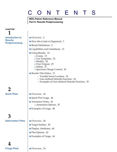
■ Overview, 2 

■ How this Guide is Organized, 3 

■ Result Definitions, 5 

2 

Quick Plots ■ Overview, 42 

■ Capabilities and Limitations, 13 

■ Using Results, 14 

❑ Create, 15 

❑ Use Templates, 23 

❑ Modify, 24 

❑ Post/Unpost, 25 

❑ Delete, 27 

❑ Spectrum/Range Control, 29 

■ Results Title Editor, 31 

- Variable Insert Location, 34 

- User-defined Defaults Function, 34 

- Examples of User-defined Defaults Function, 35 

■ Quick Plot Usage, 44 

■ Animation Notes, 46 

❑ Animation Options, 47 

■ Examples of Usage, 48 

3 

Deformation Plots ■ Overview, 56 

■ Target Entities, 58 

■ Display Attributes, 60 

■ Plot Options, 62 


4 

Fringe Plots ■ Overview, 74 

MSC.Patran Reference Manual, 

Part 6: Results Postprocessing





5 

Contour Line Plots ■ Overview, 90 




■ Contour Plot Example, 97 

6 

Marker Plots ■ Overview, 102 





7 

Cursor Plots ■ Overview, 122 

❑ Creating and Modifying a Cursor Plot, 124 

❑ Cursor Data Form, 126 

❑ Cursor Report Setup, 127 

- Cursor Report Format, 128 

- Sorting Options, 134 




8 

Graph (XY) Plots ■ Overview, 146 


- Create a Cursor Plot of von Mises Stress, 139 




■ Examples of Usage, 156

9 

Animation ■ Overview, 166 

■ Animation Options, 168 

■ Animation Control, 170 

■ Animating Existing Plots, 171 


10 

Reports ■ Overview, 176 



■ Report Options, 188 


11 

Create Results ■ Overview, 202 

■ Combined Results, 203 

■ Derived Results, 205 

■ Demo Results, 214 


12 

Freebody Plots ■ Overview, 222 

■ Select Results, 228 



■ Create Loads or Boundary Conditions, 235 

■ Tabular Display, 237 


13 

Insight ■ Overview of the Insight Application, 248 

❑ Definitions, 248 

❑ Capabilities and Limitations, 253 

■ Using Insight, 254 

■ Insight Forms, 256 

❑ Insight Imaging, 256

14 

Numerical 

Methods 

- Create, 257 

- Modify, 258 

- Delete, 259 

- Results Selection, 260 

- Animation Attributes, 261 

- Result Options, 262 

- Result Options Form, 263 

- Isovalue Setup, 264 

- Isosurface Coordinate Selection, 265 

- Tool Attributes, 266 

- Isosurface Attributes, 267 

- Isosurface Attributes Form, 267 

- Streamline Attributes, 268 

- Streamsurface Attributes, 269 

- Threshold Attributes, 270 

- Fringe Attributes, 271 

- Contour Attributes, 272 

- Element Attributes, 272 

- Tensor Attributes, 273 

- Vector Attributes, 274 

- Marker Attributes, 275 

- Value Attributes, 275 

- Deformation Attributes, 276 

- Cursor Attributes, 276 

❑ Insight Control, 277 

- Post/Unpost Tools, 277 

- Named Postings, 278 

- Isosurface Control, 279 

- Range Control, 280 

- Animation Control, 281 

- Animation Setup, 282 

- Modal Animation, 284 

- Rake Specification, 284 

- Cursor Results, 285 

- Cursor Results to File, 286 

- Cursor Results File Format, 287 

- Cursor Results File Sorting, 288 

❑ Global Settings, 288 

- Insight Spectrum, 289 

- Insight Preferences, 289 

- Insight Preferences Form, 290 

■ Introduction, 292 

■ Result Case(s) and Definitions, 293 

■ Derivations, 298 

■ Averaging, 304 

■ Extrapolation, 311 

■ Coordinate Systems, 317

15 

Verification and 

Validation 


Validation 

15 

■ Overview, 326 

■ Validation Problems, 330 

❑ Problem 1: Linear Statics, Rigid Frame Analysis, 330 

❑ Problem 2: Linear Statics, Cross-Ply Composite Plate Analysis, 335 

❑ Problem 3: Linear Statics, Principal Stress and Stress Transformation, 343 

❑ Problem 4: Linear Statics, Plane Strain with 2D Solids, 352 

❑ Problem 5: Linear Statics, 2D Shells in Spherical Coordinates, 358 

❑ Problem 6: Linear Statics, 2D Axisymmetric Solids, 363 

❑ Problem 7: Linear Statics, 3D Solids and Cylindrical Coordinate 

Frames, 372 

❑ Problem 8: Linear Statics, Pinned Truss Analysis, 378 

❑ Problem 9: Nonlinear Statics, Large Deflection Effects, 383 

❑ Problem 10: Linear Statics, Thermal Stress with Solids, 387 

❑ Problem 11: Superposition of Linear Static Results, 391 

❑ Problem 12: Nonlinear Statics, Post-Buckled Column, 401 

❑ Problem 13: Nonlinear Statics, Beams with Gap Elements, 408 

❑ Problem 14: Normal Modes, Point Masses and Linear Springs, 411 

❑ Problem 15: Normal Modes, Shells and Cylindrical Coordinates, 415 

❑ Problem 16: Normal Modes, Pshells and Cylindrical Coordinates, 421 

❑ Problem 17: Buckling, shells and Cylindrical Coordinates, 426 

❑ Problem 18: Buckling, Flat Plates, 429 

❑ Problem 19: Direct Transient Response, Solids and Cylindrical 

Coordinates, 432 

❑ Problem 20:Modal Transient Response with Guyan Reduction and Bars, 

Springs, Concentrated Masses and Rigid Body Elements, 436 

❑ Problem 21: Direct Nonlinear Transient, Stress Wave Propagation with 1D 

Elements, 442 

❑ Problem 22: Direct Nonlinear Transient, Impact with 1D, Concentrated 

Mass and Gap Elements, 447 

❑ Problem 23: Direct Frequency Response, Eccentric Rotating Mass with 

Variable Damping, 452 

❑ Problem 24: Modal Frequency Response, Enforced Base Motion with Modal 

Damping and Rigid Body Elements, 456 

❑ Problem 25:Modal Frequency Response, Enforced Base Motion with Modal 

Damping and Shell P-Elements, 462 

❑ Problem 26: Complex Modes, Direct Method, 465 

❑ Problem 27: Steady State Heat Transfer, Multiple Cavity Enclosure 

Radiation, 471 

❑ Problem 28: Transient Heat Transfer with Phase Change, 475 

❑ Problem 29: Steady State Heat Transfer, 1D Conduction and 

Convection, 479 

❑ Problem 30: Freebody Loads, Pinned Truss Analysis, 482 

INDEX ■ MSC.Patran Reference Manual, 487 

Part 6: Results Postprocessing

MSC.Patran Reference Manual, Part 6: Results Postprocessing 

CHAPTER 

1 

Introduction to Results 


■ Overview 

■ How this Guide is Organized 

■ Result Definitions 

■ Capabilities and Limitations 

■ Using Results 

■ Results Title Editor

PART 6 

Results Postprocessing 

1.1 Overview 

The MSC.Patran Results application gives users control of powerful graphical capabilities to 

display results quantities in a variety of ways: 

• Deformed structural plots 

Color banded fringe plots 

Contour line plots 

Marker plots (scalars, vectors, tensors) 

Cursor plots 

Freebody diagrams 

Graph (XY) plots 

Animations of most of these plot types. 

The Results application treats all results quantities in a very flexible and general manner. In 

addition, for maximum flexibility results can be: 

Sorted 

Reported 

Scaled 

Combined 

Filtered 

Derived 

Deleted 

All of these features help give meaningful insight into results interpretation of engineering 

problems that would otherwise be difficult at best. 

The Results application is object oriented, providing postprocessing plots which are created, 

displayed, and manipulated to obtain rapid insight into the nature of results data. The imaging 

is intended to provide graphics performance sufficient for real time manipulation. Performance 

will vary depending on hardware, but consistency of functionality is maintained as much as 

possible across all supported display devices. 

Capabilities for interactive results postprocessing also exist. Advanced visualization capabilities 

allow creation of many plot types which can be saved, simultaneously plotted, and interactively 

manipulated with results quantities reported at the click of the mouse button to better 

understand mechanical behavior. Once defined, the visualization plots remain in the database 

for immediate access and provide the means for results manipulation and review in a consistent 

and easy to use manner.

1.2 How this Guide is Organized 

The Guide is broken into the following chapters to provide a logical flow. 

Introduction to Results 


CHAPTER 1 

Introduction to Results Postprocessing 

An overview of the Results application. It is important that first time 

users read this thoroughly to fully understand how the Results 

application works. Important definitions are defined to understand 

how results data are stored in the database and how they are 

manipulated by the Results application. An overview of the 

operation of the Results application is also provided to give a basic 

understanding of how to create and modify result plots and how to 

post/unpost or delete existing plots and results data. 

Quick Plots Eighty to ninety percent of all postprocessing needs are accessed 

through the default Results application form. This chapter explains 

the Results application default form and how to create quick fringe 

plots of any scalar data and quick structural static deformation plots 

and modal style animations and combinations thereof. 

Deformation Plots Detailed explanations of how to create and modify deformation 

plots as well as how to change display attributes, target entities and 

other options. 

Fringe Plots Detailed explanations of how to create and modify deformation 

plots as well as how to change display attributes, target entities and 


Contour Line Plots Detailed explanations of how to create and modify contour line plots 

as well as how to change display attributes, target entities and other 

options. 

Marker Plots Detailed explanations of how to create and modify marker plots 

(scalar, vector and tensor plots) as well as how to change display 

attributes, target entities and other options. 

Cursor Plots Detailed explanations of how to create and modify cursor plots as 

well as how to change display attributes, target entities and other 

options. Also instructions on how to create a report from the cursor 

plot. 

Graph (XY) Plots Detailed explanations of how to create and modify graph (XY) plots 

(including beam data) as well as how to change display attributes, 

target entities and other options. 

Animation Detailed explanations of how to create and manipulate animations 

of most plot types as well as how to change display attributes and 


Reports Detailed explanations of how to create and display reports of results 

data as well as how to change report formats and other options. 

Create Results Detailed explanations of how to derive, combine and scale results 

data as well as how to select target entities, define transformation, 

derivations and other options. 

3

PART 6 


Freebody Plots Explains the capability to graphically display freebody diagrams 

and create new loads and boundary conditions from MSC.Nastran 

grid point force balance results. 

Insight Detailed explanation of the Insight application (another MSC.Patran 

postprocessor). This postprocessor has much of the same 

functionality as the Results application with the exception of results 

derivations/combinations, reports, graphs, and freebody. However 

the Insight application allows for some additional advanced 

postprocessing tools such as isosurface, scalar icon, value, cursor, 

and streamline plots. 

Numerical Methods Detailed explanations of the many numerical manipulations that are 

exercised in the Results application. These include operations such 

as vector and tensor to scalar calculations, extrapolation methods, 

coordinate transformations, results derivations and averaging 

techniques. 


Validation 

Verification and Validation problems are presented to validate and 

verify postprocessing displays using standard and widely accepted 

engineering problems. This is also a good source of example 

problems for learning to use the Results application.

1.3 Result Definitions 

CHAPTER 1 


In order to fully utilize the power of the postprocessor, a thorough understanding of how the 

results are stored and manipulated is important. To avoid confusion or the possibility of 

misinterpreting the graphical displays, the following definitions should be understood. 

Result Types. There are really only three results types, either scalar, vector, or tensor. Aside 

from these there are other aspects of results data as stored in the database that need to be 

understood. The following table summarizes these: 

Term Description 

Nodes/Elements Results are associated with either nodes or with elements. 

Scalar Results 

Vector Results 

Tensor Results 

Real/Complex 

Number 

Load Case 

Results Case 

Single results values associated with either nodes or elements. They 

contain a magnitude only with no direction. Examples: strain energy, 

temperature, von Mises stress, etc. 

Results values with three (3) components each associated with either 

nodes or elements. Vector results contain both magnitude and 

direction Examples: displacement, velocity, acceleration, reaction 

forces, etc. 

Results values with six (6) components each (typically comprising 

the upper triangular portion of a symmetric matrix) associated with 

either nodes or elements. Examples: stress and strain components 

Results stored as real numbers have only single values associated 

with any node or element. Complex numbers have two values 

associated with any node or element and are stored in the database 

as real and imaginary parts or magnitude and phase. 

A group of applied loads and boundary conditions which may 

produce one or more result cases. 

A collection of results as stored in the database (e.g., static analysis 

results, results from a load step in a nonlinear analysis, a mode shape 

from a normal mode analysis, a time step from a transient analysis, 

etc.). 

Result Type Either scalar, vector, or tensor. Scalar results contain a magnitude 

with no direction such as temperature, strain energy, von Mises 

stress, etc. Vector results contain both magnitude and direction, such 

as displacement, velocity, and acceleration. Tensor results are 

symmetric with six unique values (xx, yy, zz, xy, yz, zx) such as stress 

or strain at a point. Each Results Case can have many Results types in 

them. 

Global Variables 

Values associated with results cases as a whole rather than to 

individual nodes and elements. Each result case may be associated 

with zero, one or more global variables, (e.g. time, frequency, load 

case, etc.). 

5

PART 6 


Term Description 

Primary Results 

Layer Positions 

Element Positions 

Physical quantities which may contain several different secondary 

result types. For example, stress is a primary result and von Mises 

stress is a derived or secondary result. 

The location where element results are computed for plates and 

shells which may be homogenous or laminated. Other types of 

elements have a default non-layered ID. Beam results can also be 

layered. Examples are top, bottom, and middle results of plate 

elements, different locations in a beam cross section, etc. 

The location within the element (at a particular layered position for 

plates, shells, and beams) where results are computed. These 

positions are the quadrature points, element centroid, or nodal 

points. For beam plots, results at intermediate points along the beam 

can also be displayed as long as the analysis code has computed 

results at those locations. 

When postprocessing results, you should be able to answer these questions about any data that 

is to be evaluated: 

Is the result type scalar, vector, or tensor? 

Is the result associated with nodes or elements? 

Is the result single-valued or complex (real/imaginary)? 

What layer-position does the result belong to? 

For element results, where in the element is the result computed? 

Plot Definitions. The Results application provides various different plot types for results 

visualization. These plots, sometimes referred to as tools or plot tools, allow graphical 

examination of analysis results using a variety of imaging techniques and also simultaneous 

display of multiple plots to aid in the understanding of interactions between results. The 

following table summarizes the plots available followed by a description of each. 

Plot Type Description 

Deformation Plots Display of the model in a deformed state. 

Fringe Plots Contoured bands of color representing ranges of results value. 

Contour Line Plots Colored contour lines representing result values. 

Marker Plots Colored scaled symbols representing scalar, vector and tensor plots. 

Cursor Plots Labels for scalar, vector or tensor quantities are displayed on the 

model at interactively selected entities. 

Animation Not technically a plot type, however most plot types can be animated 

in a modal or ramped style or in a transient state if more than one 

result case is associated with an particular plot type. 

Freebody Plots These are freebody diagrams plotted specifically from MSC.Nastran 

grid point force balance results.

Plot Type Description 

CHAPTER 1 


Graph (XY) Plots XY plots of results versus various quantities. Results can be plotted 

against other results values, distances, global variables or arbitrary 

paths defined by geometric definitions such as a curve. 

Reports Also not technically a plot type, however report definitions of results 

are stored in the database like any other plot tool type and can be 

created and modified to write reports to text files or to the screen. 

Deformation plots are used to display the current model and posted plot tools in a deformed 

state. Care must be taken when applying other plots on a deformation plot when more than one 

deformation plot is posted since multiple deformation plots can easily clutter the graphics. An 

optional display of an undeformed model is controlled as an attribute of the deformation tool. 

The targeting of deformation tools to anything other than nodes and elements or groups of 

nodes and element is not allowable. Deformations may be used to display any nodal vector data. 

Fringe plots map color to surfaces or edges based on the result data defined for the tool. Fringes 

are developed from nodal-averaged scalar values. Fringes may be plotted on the model’s 

element faces or edges. The fringe tool will supersede all existing or default color and shading 

definition for the entities at which the fringe is targeted. 

Contour Line plots display contour lines representing result data selected. Contours line plots 

are developed from nodal-averaged scalar values. Contour lines may be plotted on the model’s 

element faces or edges. 

Marker plots display nodal or element based scalar, vector or tensor results as icons or arrows 

at the result locations. Markers may be targeted at model features such as nodes, corners, and 

edges or faces of elements. Individual scalar, vector and tensor plots are described below but are 

known generically as marker plots. 

Cursor plots display nodal or element based scalar, vector or tensor results as labels. There are 

three types of cursor plots: (1) Scalar, (2) Vector or (3) Tensor. Scalar, vector and tensor result 

quantities are displayed as one, three and six labels, respectively. Labels may be targeted at 

model features such as nodes and elements. Cursor plots are interactive and the labels are 

displayed on the model as the user selects the entities. The result value labels maybe displayed 

in a spreadsheet and written to a file, if desired. 

Scalar plots display nodal or element based scalar data and are considered special types of 

marker plots. Scalars may be colored and scaled based on value and may be targeted at various 

model features such as node, faces and edges of elements, and corners. 

Vector plots display nodal or element based vector data as component or resultant vectors and 

are considered special types of marker plots. Vectors may be colored and scaled based on 

magnitude and may be targeted at various model features such as node, faces and edges of 

elements, and corners. 

Tensor plots display an iconic representation of a symmetric tensor and are considered a special 

type of marker plot. Tensors may be oriented in the axes of principal stress or the tensor’s 

defined coordinate system. Tensors may be defined by element- or nodal-based tensor data. 

Nodal tensors are mapped from element tensors and are used when a tensor marker tool is 

targeted at other tools. Tensors may be targeted at nodal- and element-based model features. 

7

PART 6 


Animation of most plot types is fully supported. Deformations can be animated in modal or 

ramped styles as well as true deformations from transient analyses. Animations from other plot 

types can accompany a deformation animation such as a stress field fringe plot or they can be 

animated separately from the deformation. Animation can be turned on or off from any existing 

plot or can be designated at creation time or when modifying a plot. The number of animation 

frames and other parameters such as the speed of animation are all easily controllable. 

Freebody plots display a freebody diagram on a selected portion of the model. The plots are in 

the form of vector plots showing either the individual components or resultant values. 

Individual components that make up the total freebody diagram can also be plotted separately 

such as reaction forces, nodal equivalenced applied forces, internal element forces and other 

forces such as those from MPCs, rigid bars, or other external influences. New loads and 

boundary condition sets can be created from a freebody plot. 

Graph plots are XY plots generally consisting of a results value versus some variable such as 

time or frequency or possibly a model attribute such as distance from a hole or edge or another 

results value. 

Plot Attributes. The Results application provides the means of Creating, Modifying, Deleting, 

Posting and Unposting these plots as well as means for dynamically manipulating these plots 

for interactive results imaging. Each plot created has assigned attributes which determine its 

characteristics. All plots have the following attributes. 

Attribute Description 

Name A unique user-definable string descriptor to identify the plot tool. If no 

plot name is specified a default name is used. The default will be used 

each time unless the user specifically defines a unique name. 

Type One of the plot tool types described in Plot Definitions (p. 6). 

Result(s) A results case or a list of results cases and the corresponding result type 

which the plot tool is to display. 

Target Onto where or to what entities the plot is to be displayed. This is either 

on a model feature such as nodes, elements, or on another plot tool. 

Display 

Attributes 

Animation 

Attributes 

Each plot type has specific settings to control how the plot is to be 

displayed. These include such things as component colors, titles, label, 

rendering styles and a myriad of other attributes. 

Attributes to describe whether the tool is to be animated and how the 

results are to be mapped to animation frames. For instance, is the 

animation modal or transient and how many frames will be used for the 

animation? 

Posting Status Each plot is either Posted (displayed) or Unposted (not displayed) with 

the exception of reports. 

Plot Targets. Result plots may be displayed on selected model entities or other selected plot 

tools. The model based targets may be defined by a list of posted groups, by all posted entities 

in the current viewport, or by individual nodes or elements or by elements with certain 

attributes. The model entities and tools which may act as targets for Results application plots are 

described below.

CHAPTER 1 


Elements indicate that results will be displayed on all selected elements of the model. For 

graphs and reports the information can be extracted from the centroid, the element nodes or 

element data as stored in the database. 

Free faces describe those element faces common to only one element. This includes faces lining 

the outside surface of a model or those inside surfaces exposed to internal voids. Free faces are 

appropriate targets for displays such as fringe plots which are normally displayed on the surface 

of the model or on a cutting plane through the model. 

All Faces display results on each face of each element. 

Free Edges display results on edges common to only one element. Use this target type when 

displaying results on the same edges which are used to draw the model when Free Edge is 

selected as the finite element display method. 

All Edges display results on all element edges. Using this target selection allows mapping of 

results onto a wireframe representation of the model. 

Nodes display the selected results at each nodal location of the model. Tensor and vector plots 

may all be displayed at nodal locations. 

Corners display the selected results at nodes which are common to only one element. Tensor 

and vector plots may all be displayed at corner locations. 

Paths display the selected results along a defined path. The path can be defined as either a series 

of beams or element edges, geometric curves, or selected points (either geometric or FEM based). 

This target type is used with Graphs plots. 

The following table summarizes the valid targets for all plot tools. When specifying target 

entities in most cases you must specify both the target entities to which the plot will be assigned 

and the attributes or additional display information. The table below shows target entity versus 

attribute and which plots types are valid (D=deformation, F=fringe, Cl = Contour Lines, S= 

Scalar, V=vector, T=tensor, Cu=Cursor, G=graph, R=report). 

Target 

Element 

Free Faces 

Current Viewport D,S,V,T,R F,Cl,S 

,V,T 

All Faces 

Free Edges 

F F,S,V 

,T 

Attribute 

All Edges 

Nodes 

Corners 

F D,S, V,T,R S,V, 

T 

Curves/ 

Edges/ Beams 

Nodes D,S,V,T, 

Cu,G,R 

Elements D,S,V,T, 

Cu,G,R 

F,Cl F F F R 

Groups D,S,V,T,G, 

R 

Materials D,S,V,T,G, 

R 

F,Cl,S 

,V,T 

F,Cl,S 

,V,T 

F F,S,V 

,T 

F F,S,V 

,T 

F D,S,V,T,G, 

R 

S,V, 

T 

F D,S,V,T,G S,V, 

T 

Elem. Nodes / 

All Data 

R 

G,R 

G,R 

9

PART 6 


Target 

Element 

Properties D,S,V,T,G, 

R 

Free Faces 

F,Cl,S 

,V,T 

Element Types D,S,V,T,R F,Cl,S 

,V,T 

F F,S,V 

,T 

F F,S,V 

,T 

Attribute 

F D,S,V,T,G S,V, 

T 

F D,S,V,T S,V, 

T 

Paths G 

All Faces 

Free Edges 

All Edges 

Nodes 

Corners 

Curves/ 

Edges/ Beams 

Elem. Nodes / 

All Data 

G,R 

R

Other Definitions 

Term Definition 

Post To graphically display the plot or plots. 

Unpost To remove the plot or plots from the graphical display. 

CHAPTER 1 


Range A MSC.Patran database entity defined by a series of number and 

threshold values for each level within a range. Ranges are used to 

map spectrum colors to results values. A spreadsheet form is 

available to control range levels. 

Viewport Range The range entity currently assigned to the MSC.Patran viewport. 

Auto Range A range which is not a database entity but is automatically calculated 

for a plot based on the results values. This type of range may be 

manipulated dynamically to change the range extremes and the 

number of intermediate levels. 

Extrapolation 

Averaging 

Derive 

Interpolation 

Coordinate 

Transformation 

Methods of converting results values from certain element locations 

to other locations (e.eg., converting results at Gauss points to nodal 

values). 

Methods of converting several results associated to the same physical 

location to a single results value such as when results at nodes have 

contributions from all connected elements. 

Methods of converting results values, for instance, when calculating 

von Mises stress from stress tensor components. 

Methods of calculating new results values between existing locations 

of results values. For example: displaying more frames of animations 

than results cases available. 

Methods of transforming results values with magnitude and 

direction attributes into alternate systems. 

More detailed information on the numerical methods can be found in Numerical Methods 

(Ch. 14). 

Results Label. MSC.Patran displays results labels on plots so that all labels are started at the 

free end of the line segment (away from the node or element centroid); and continue to the right, 

independent of the arrow. Often the label is obscured. 

For vector and tensor plots, you can now set the label to appear at the free end of the line 

segment, and position it so that it appears centered with respect to the arrow. All labels are 

pushed “away” from the segments (i.e., an arrow that goes from the screen center to the left will 

have the label end at the arrowhead instead of the begin at the arrowhead, as in the past). To 

enable the label placement feature, you need to add a preference to the Patran db using: 

db_add_pref(524,2,0,TRUE,0.0,"") 

db_set_pref_logical(524,TRUE) 

from the patran command window input text data box. This will remain in effect for the life of 

the database. 

1

PART 6 


When the "VECTORTEXTCENTERED" preference (524) is in effect, the label text associated to 

results vectors, result tensors, lbc marker "arrows", property "arrows", and arrow created using 

"gm_draw_result_arrow": 

are not rendered until the end of the viewport rendering. The text that is attached to an 

arrow is drawn at a location so that the free end of the vector receives the text. The hang 

point of the text is translated (in the 2d world) such that the center of the box enclosing 

the text (text box) is contained in the line of the (2d) vector and the edge of the text box 

is just touching the free end. 

are suppressed (not rendered) if the free end of the vector to which the text is attached 

is occluded. That is, if the z-depth of the device coordinate for the free endpoint is 

greater than the current z-depth for the device x,y (something eclipses the end of the 

vector tail) then the text is suppressed. This does not apply if the viewport was 

rendered entirely in wireframe mode. All vector text is considered visible if the 

viewport was rendered in wireframe mode.

1.4 Capabilities and Limitations 

CHAPTER 1 


The Results application provides the capabilities for Creating, Modifying, Deleting, Posting, 

Unposting and manipulating results visualization plots as well as viewing the finite element 

model. In addition, results can be derived, combined, scaled, interpolated, extrapolated, 

transformed, and averaged in a variety of ways, all controllable by the user. 

Control is provided for manipulating the color/range assignment and other attributes for plot 

tools, and for controlling and creating animations of static and transient results. 

Results are selected from the database and assigned to plot tools using simple forms. Results 

transformations are provided to derive scalars from vectors and tensors as well as to derive 

vectors from tensors. This allows for a wide variety of visualization tools to be used with all of 

the available results. 

Results imaging routines are optimized for graphical speed but may vary depending on 

hardware. 

Please be aware of the following limitations or constraints: 

When a Result Data quantity is deleted, it is deleted from all Results Cases that contain 

the Results Data quantity. 

Transient animations are not possible from the Quick Plot form. They must be created 

under each specific plot type option (deformation, fringe, marker, etc.). 

Multiple animations can be viewed simultaneously in a single viewport. 

Only one spectrum and range can be associated to any one viewport at a time. If 

multiple plots are posted to a viewport, the spectrum and corresponding range will 

only be applicable to one of the posted plots. Values from other plots not corresponding 

to the posted range will take on the posted range’s spectrum. Values outside the range 

will appear as the highest or lowest range color. This may make some plots appear 

monochrome. This is done to avoid confusion and misinterpretation of result data. 

It is not recommended to calculate invariants (e.g., von Mises) from complex results 

because the phase is not accounted for. 

1

PART 6 


1.5 Using Results 

The Results application is based on the creation and manipulation of results visualization plots. 

The first action to be performed using Results is to create a plot, sometimes referred to as a tool 

or a plot tool. This however is transparent to the user when doing basic operations such as 

simple deformed plots, fringes, and animation. Each plot type has its own default settings and 

attributes which are set and modified when a user creates a plot. Only when these settings and 

attributes need to be saved and restored quickly for subsequent use does the user need to 

concern himself about physically saving the plots. This is done using the Create action on the 

main Results application form. Other actions are described in the following table, and 

summarized in this section. 

Action Description 

Create This action is used to create Results visualization plots sometimes 

referred to as tools. Creating a plot will result in a graphical display 

with the exception of creating reports and deriving results. If you try 

to create a plot that already exists, you will be prompted for 

overwrite permission. 

Selecting Results 

and Filtering 


Sometime it is necessary to select only certain Results Cases or to 

filter the Results Cases specifically for more precise control when 

creating plots. A special form allows you to do this easily and 

efficiently as well as view all Results Cases available to you. 

Modify This action is used to modify existing Results visualization plots or 

tools. This action performs identically to the Create action with the 

exception that no overwrite permissions will be asked if plot tools 

already exist that are being modified. 

Post/Unpost This action is used to graphically display (post) or graphically 

remove (unpost) existing Results display plots or ranges/spectrums 

from the computer screen. The plots and ranges are not physically 

removed from the database with this operation. Only their graphical 

display is recalled or removed. 

Delete This action is used to delete existing Results visualization plots and 

for deleting result cases and result data associated with result cases 

from the database. Use this option with care. Some operations may 

not be undoable. 

Spectrum/Range 

Control 

There is a form which allows the currently posted spectrum to be 

changed and manipulated as well as deleted or new ones created. 

There is also a form which allows for control over which range 

(numbers) are assigned to newly created plots and also control over 

each color bar of the spectrum for the currently posted plot or plots. 

See Spectrum/Range Control (p. 29). 

Animation Control These are forms for setting up and controlling certain aspects of an 

animation. See Animation (Ch. 9) for details.

Create 

CHAPTER 1 


Creating a plot generally involves four to six basic steps (although it may vary from plot type to 

plot type). For simple plots where it is acceptable to use all default values then the Quick Plot 

option is all that is needed. The icons on the top of the form give access to all controls necessary. 

For full control of most plots the steps are: 

Action: 

Object: 

Results Display 

Select Result Case(s) 

Create 

Deformation 

Load Case 1, Static Subcase 

Select Deformation Result 

Applied Loads, Translational 

Displacements, Translational 

Displacements, Rotational 

Show As: 

Animate 

-Apply- 

Resultant 

Reset All 

Note: A separate chapter is dedicated 

to describe in detail the creation and 

manipulation of each plot type. 

STEP 1: Set the Action to Create and select an 

Object (the plot type) from the Results application 

form. 

STEP 2: Select a Results Case from this listbox. 

STEP 3: Select a result associated with the Results 

Case from this listbox. 

STEP 4: Select the target entities to which the plot 

will be applied (optional). 

STEP 5: Set any plot attributes if necessary 

(optional). 

STEP 6: Press the Apply button on the bottom of the 

form. The plot will be displayed. 

☞ More Help: 

Plot Types: 

• Quick Plots (Ch. 2) 

Deformation Plots (Ch. 3) 

Fringe Plots (Ch. 4) 

Contour Line Plots (Ch. 5) 

Marker Plots (Scalar, Tensor, Vector) 

(Ch. 6) 

Cursor Plots (Ch. 7) 

Graph (XY) Plots (Ch. 8) 

Animation (Ch. 9) 

Reports (Ch. 10) 

Create Results (Ch. 11) 

Important: Plots can be optionally named and saved in the database and subsequently 

recalled and graphically displayed. If no name is given, a default name is 

assigned. If a new plot is created without specifying a name, the default will be 

overwritten each time. Overwrite permission will be asked if a name is given and 

it already exists. 

1

PART 6 


Selecting Results. For all operations you must select results from a listbox. What results are 

displayed in this listbox is somewhat dependent on the result type (static, transient, etc.) or the 

number of subcases, time, frequency, or load steps associated with these results and how they 

have been filtered. When multiple subcases, time, frequency, or load steps are present, the 

display in the Select Result Cases listbox will display a title such as LoadCase x, n of n subcases 

or something similar indicating that there are multiple sets of results for this Result Case. 

When multiple results exist for any given Result Case, an additional button and toggle appear 

on the form. One allows for filtering and selecting the desired subcases which will appear 

selected in the listbox and the other determines the appearance of these multiple results in the 

listbox itself. 

Action: 

Object: 


Select Result Cases 

Create 

Load Case 1, 1 of 41 Subcases 





Show As: 

Fringe 

Position...(At Z1) 

Animate 

-Apply- 

Resultant 

Reset All 

This button icon brings up the Select Result Cases form to 

allow for selecting and filtering of the results cases based on 

various criteria such as a global variable (time). Once the 

filtering has been done only those results that passed the 

filter criteria will be selected for subsequent postprocessing. 

See Filtering Results (p. 19). 

This button icon changes the way the Result Cases are 

displayed in the listbox. If toggled OFF, every individual 

subcase, time, frequency, or load step will be visible in the 

listbox. If toggled ON, then only the title of the primary Result 

Case will appear with a summary of how many subcases are 

associated with it based on the filter criteria. This is known as 

the abbreviated form. 

This toggle will not appear unless Result Cases with multiple 

subcases exist. This is true also for the Select button icon. 

Additional results selection control is given when multiple 

layers exist. 

Once Result Cases have been selected and filtered, the Result Case name will be updated to show 

how many subsets of that Result Case have been selected. The name will appear something 

similar to LoadCase x, m of n subcases. If the Abbreviate Subcases toggle is then turned OFF, 

only those subcases selected through the filtering mechanism will be highlighted in the listbox. 

How to filter results is explained in Filtering Results (p. 19). 

Be aware that when selecting multiple Result Cases, such as for a transient animation, that the 

selected result type to plot must exist in all Result Cases selected. Otherwise an error message 

will result and no plot will be displayed until the Result Case selection is modified to meet this 

criterion.

CHAPTER 1 


Result Layer Positions. When multiple layers exist in a given result type, this form may be 

invoked by pressing the Position button in the Results application when the mode is set to Select 

Results. Layers may correspond to shell top/bottom, ply layups, or different element type 

results. 

At Point C 

At Point D 

At Point E 

At Point F 

At Z1 

At Z2 

Select... 

Positions 

Option: Maximum 

Close 

This form is accessible by pressing the Position 

button from the Select Results mode if multiple 

layers exist for a given result type. 


Select the position(s) you wish to be used in any subsequent 

plot. You may select multiple layers for any single Result 

Case or you may pick a single layer for use when a single or 

multiple Result Cases are selected. 

Set the option to search and extract result quantities when 

multiple layers or Result Cases have been selected. These 

options are explained in the table below. 

Maximum If multiple layers or multiple Result Cases have been selected, then 

this option will search through all layers/Result Cases and extract 

the maximum value encountered for the subsequent plot. The value 

used in the search is the Quantity selected for resolution such as 

von Mises for tensor results. 

Minimum This is identical to Maximum except the minimum is extracted. 

Average Instead of extracting a maximum or minimum, values are averaged 

from each layer or Result Case based on the Quantity selected and 

graphically reported. Averaging is only performed over the 

number of actual layers or Result Cases that contained results at 

any entity. That is if 4 layers were selected and node 1 had three 

layers of results and node 4 had four layers of results, node 1 would 

be averaged only over the three that actually existed and not the 

four selected. 

Sum This option simply sums all values of the requested Quantity from 

each layer or Result Case and reports that value in the subsequent 

plot. 

Merge This option will use the first existing value encountered from any 

particular layer or Result Case. For instance if both top and bottom 

stresses are selected then only the top will be reported. This is 

useful for layers that are associated with certain element types. 

That way a layer with shells, a layer with solid, and a layer with 

beam elements can all be displayed simultaneously on the graphics 

screen in one operation. 

1

PART 6 


Note that when performing maximum/minimum extractions or averaging and summing that 

the following procedures are performed in order: 

1. The selected Quantity of interest is calculated for all layers or Result Cases 

selected, first performing any transformations, scaling, and averaging, or 

extrapolation as requested in the Plot Options. Quick Plot operations use 

standard defaults for all plot options. 

2. Once the Quantity of interest is calculated for all selected layers or Result Cases, the 

maximum/minimum extraction, averaging or summation is performed and reported 

in the subsequent plot. 

Note that this operation is different than what the results derivations do in Derived 

Results (p. 193). These operations are scalar based, meaning that the maximum, 

minimum, average, or sum operations are done based on the requested scalar 

quantity.For instance, you would not be able to properly calculate von Mises stress at 

the neutral axis of a beam in pure bending by selecting the top and bottom layers and 

requesting an average where the expected von Mises stress should be zero. The von 

Mises will be calculated at top and bottom and then averaged. For this type of 

operation where the components of a vector/tensor need to be averaged or summed 

before the requested result quantity is calculated or the vector/tensor components 

based on maximum or minimum comparisons of the requested scalar quantity are 

required, you must use Derived Results (p. 193). 

Important: It is important to note that if multiple Result Cases have been selected 

and only a single layer exists or has been selected that the default plot 

will result in a maximum plot of all selected results.

CHAPTER 1 


Filtering Results. Filtering results is accomplished from the Select Result Cases 

form which is accessible from the Results application when the first icon button 

(Select Results) is active and multiple subcases exists. An icon button appears 

when Result Cases are in their abbreviated form to access the filter form which can also be 

accessed by clicking on the Result Case name. 

Select Results Cases 


Load Case 1, 41 subcases 

Filter Method: Global Variable 

Variable: 

Time Min: 0. Max: 2. 

Values: Above Value: 1 

Filter 

Selected Result Cases 

Load Case 1, Time = 0. 

Load Case 1, Time = 0.05 






Clear Remove 

Apply Close 

Select a Result Case from this listbox which 

appears as a title with the number of subcases 

associated with the Result Case(s). Only one 

can be operated on at a time. 

Select a method of filtering. The methods to 

choose from are Global Variable, String, Subcase 

Ids, and All. These are described in Table 1-1. 

Set the appropriate criteria depending on the 

Filter Method above. 

Filters the subcases. The listbox below will fill with 

the selected subcases. 

Any subcases highlighted in the listbox below can 

be removed by using this button. 

Clears the Selected Result Cases listbox. 

Every time the Filter button is pressed, new 

results subcases will be added to whatever 

existing results are already selected. To do a new 

filter you must clear this listbox. 

Makes the selected subcases active for 

postprocessing. The number of selected subcases 

will appear back on the main form. Use the Close 

button to close the form down. 

This form is expandable to allow you to view the entire Result Case names and global variable 

if necessary. 

1

PART 6 


The different filter methods are explained in Table 1-1. 

Note on Result Case Names: 

Table 1-1 Filter Methods 

Method Description 

Global Variable Any global variables associated with the selected Result Case will 

show up in the Variable option menu. Select the one you would like 

to filter with, change the criteria using the Value option menu and 

enter the value or range to filter by. Press the Filter button to 

complete the filter action. Press the Apply button at the bottom of 

the form to activate the filtered subcase selection. 

String Enter a string and use wild cards (the * character) to filter results. 

For example if you wanted all subcases with the string Time in it 

then you would use *Time* as the string with wild cards on each 

end of the word. Press the Apply button at the bottom of the form 

to activate the filtered subcase selection. 

Subcase IDs Subcases can be filtered on Subcase IDs by entering the appropriate 

IDs. To select separate IDs, separate them by spaces (1 3 5). To select 

a range use a colon between the numbers (1:5). To select by 

increments use two colons, for example: 1:10:2, which interpreted 

means select subcases one through 10 by twos. Or use any 

combination of spaces and colons between subcase IDs to select as 

many as you wish. Press the Apply button at the bottom of the 

form to activate the filtered subcase selection. 

All No filter method is selected. No options are available. Simply press 

filter and all subcases will be selected from whatever primary 

Result Case is selected. Press the Apply button at the bottom of the 

form to activate the filtered subcase selection. 

Important: Only one Result Case can be filtered at a time. If you need to filter subcases from 

more than one Result Case then you will need to perform the operation once for 

each Result Case. 

By default if a Result Case has more than 30 subcases (time steps, load steps, etc.) then the 

Result Case name will be displayed in an abbreviated form to reduce clutter in the 

listboxes. The default number at which this abbreviated form takes over can be changed 

with a settings.pcl parameter: 

pref_env_set_integer( “result_loadcase_abbreviate”, 30 ) 

See The settings.pcl file (p. 41) in the MSC.Patran Reference Manual, Part 1: Basic Functions. It is 

possible to toggle back and forth from abbreviated form and full form at any time by pressing 

the icon button shown here.

CHAPTER 1 


Default Settings. For all modes of the Results application (selecting results, target entities, 

display attributes, plot options, and animation options) logical defaults have been set. In general, 

when an option on a form is changed, it remains until the user modifies or resets it. On the 

bottom of the Results application form is a Reset button that will restore default settings. 

Pressing the Reset button only affects the particular plot type currently set. 

-Apply- Reset All -Apply- Reset 

In the Select Results mode of the 

Results application, the Reset All button 

will restore all default settings for any 

particular plot type. This includes target 

entities, display attributes, plot and animation 

options. 

In any other mode of 

the Results 

application, the 

Reset button will only 

restore that modes settings for any particular plot type. 

In some instances it is possible to modify these defaults to the user’s preference. Not all default 

attributes and setting can be altered by the user since certain dependencies exist on result types 

and available options. However for display attributes, default setting may be altered in a 

template database. This template database can then be saved and made available to all users that 

wish to use the altered default attributes. See The Template Database File (template.db) (p. 47) 

in the MSC.Patran Reference Manual, Part 1: Basic Functions 

In order to accomplish this, the standard MSC.Patran database is pre-loaded with invisible plot 

tools called MSC_Initialize. There is one for each plot type (Deformation, Fringe, Vector, 

Tensor, Graph). This plot is never visible to the user but default display attributes are extracted 

from these plot tools. 

Toggles the form to change display attributes for all plot types. 

To modify the default display attributes, you simply need to modify the MSC_Initialize plot 

tool for the plot type in question. These basic steps need to be followed: 

1. Open a MSC.Patran database that already has a model and results or simply create a 

new database and model using Demo results (See Demo Results (p. 202).) 

2. Create a plot of the type you wish to modify with the display attributes that you want. 

A PCL command will be issued in the command line window of MSC.Patran. It will 

also be output to a session file typically called patran.ses.01 (the version number may 

vary). 

3. Either edit the session file or edit the PCL command from the command line by 

replacing the plot name (which will probably be blank something like default_XXX 

where XXX is Fringe, Tensor, Vector, etc.) with the name MSC_Initialize. See the 

example below. 

4. Also edit this PCL command such that it is a modify command as opposed to a create 

command. 

5. Close down the current database and open a new blank database. 

2

PART 6 


6. Run the edited session file or re-issue the PCL command to modify the MSC_Initialize 

plot tool. 

7. Save this database as the new template.db. 

Display attributes for this modified plot tool have now been set. 

As an example, say that the default display attributes for a deformation plot are to be modified. 

The following PCL command is issued when creating a deformation plot with the desired 

attributes: 

res_display_deformation_create(““,“Elements”,0,[““],9,[“DeformedStyle:White,Solid,1,Wire 

frame”,“DeformedScale:Model=0.1”,“UndeformedStyle:ON,Blue,Dash,1,Wireframe”,“TitleDispla 

y:ON”,“MinMaxDisplay:ON”,“ScaleFactor:1.”,“LabelStyle:Fixed,8,White,4”,“DeformDisplay:Re 

sultant”,“DeformComps:OFF,OFF,OFF”]) 

The PCL command should then be edited as follows: 

res_display_deformation_modify(“MSC_Initialize“,“MSC_Initialize”,“Elements”,0,[““],9,[“D 

eformedStyle:White,Solid,1,Wireframe”,“DeformedScale:Model=0.1”,“UndeformedStyle:ON,Blue 

,Dash,1,Wireframe”,“TitleDisplay:ON”,“MinMaxDisplay:ON”,“ScaleFactor:1.”,“LabelStyle:Fix 

ed,8,White,4”,“DeformDisplay:Resultant”,“DeformComps:OFF,OFF,OFF”]) 

Note that the only modifications are to change the create to modify in the PCL function name and 

enter the name of the plot tool MSC_Initialize twice. This PCL command should then be issued 

either via a session file or directly from the command line after opening a new empty database. 

The above example simply sets the undeformed line style to dashed as opposed to the standard 

solid line.

Use Templates 

CHAPTER 1 


This Action menu provides the means to select and use Results Templates to make Deformation 

Plots, Fringe Plots, Marker Vector Plots, Marker Tensor Plots, Graphs, and Reports. 

The menu is similar to the Create menus, except that the Results Display Attributes and Plot 

Options icons and associated menus have been replaced with a Display Templates icon and 

associated menu. The Display Attributes and Plot Options values will be determined by the 

Results Template selected instead of the many individual menu settings on the Display 

Attributes and Plot Options forms of the Create menu. 

For Results plots (Deformation, Fringe, Marker Vector and Marker Tensor) you may chose a title 

either from the template or as determined by the load selection on the Select Results form. Either 

can be edited once selected by the corresponding switch for “Title From:” “Template” or “Load 

Selection”. 

Graphs do not use titles. 

Report Titles are accessed via the “Format…” button. 

STEP 1: Set the Action to Use Template. 

STEP 2: Select the type of plot for which you will 

use a template. 

STEP 3: Change the Result Cases and/or results 

type assigned to this plot (optional). 

STEP 4: Select to show as either Resultant or 

Component. 


form. 

2

PART 6 


Modify 

Once a plot has been created, it may be modified using the Modify action on the Results 

application form. It is only necessary to actually modify a plot if it has been optionally named 

and saved in the database. Otherwise the Create action can be used exclusively. Default plots can 

be overwritten with the Create action. To modify a named plot, follow these general steps: 

Action: 

Object: 

Load Case 1 

Load Case 2 

Load Case 3 


Modify 

Deformation 

Existing Deformation Plots... 



Deformation, Translational 

Deformation, Rotational 

Show As: 

Animate 

-Apply- 

Resultant 

Reset All 

Note: A separate chapter is dedicated 

to describe in detail the creation and 

modification of each plot type. 

STEP 1: Set the Action to Modify and select an Object 

(the plot type) from the Results application form. 

STEP 2: Select the named plot to be modified. 

STEP 3: Change the Result Cases and/or results type 

assigned to this plot (optional). 

STEP 4: Change the target entities to which the plot will 

be applied (optional). 

STEP 5: Modify the plot attributes and other options if 

desired (optional). 


form. The plot will be modified and displayed if not 

already. 

☞ More Help: 

Plot Types: 

Quick Plots (Ch. 2) 

Deformation Plots (Ch. 3) 

Fringe Plots (Ch. 4) 

Contour Line Plots (Ch. 5) 

Marker Plots (Scalar, Tensor, Vector) 

(Ch. 6) 

Cursor Plots (Ch. 7) 

Graph (XY) Plots (Ch. 8) 

Animation (Ch. 9) 

Reports (Ch. 10) 

Create Results (Ch. 11) 

Important: It is suggested to only modify plots that have specifically been given names. It is 

not necessary to modify the default plots. Default names are given to the plots 

when no specific name is specified. The Create action continually overwrites 

these default plots with their corresponding names, therefore it is not necessary to 

use the Modify action on them.

Post/Unpost 

CHAPTER 1 


Posting and unposting of plots to the graphics viewport(s) can be performed. Posting or 

unposting of ranges and their corresponding spectrum is also allowable. See the next section 

Posting/Unposting Ranges (p. 26). 

Posting/Unposting Plots. Once a plot or set of plots has been created, they may be posted 

(displayed) or unposted (removed) with the Post action on the Results application form. (This is 

also true for Ranges. SeePosting/Unposting Ranges (p. 26) and Spectrum/Range Control 

(p. 29) for more detail. Multiple plots may be posted simultaneously. To post or unpost a plot, 

do the following: 

Action: 

Object: 


Existing Plot Types 

Post 

Plots 

DEF_default_Deformation 

FRI_default_Fringe 

VEC_default_Vector 

Select None 

Select All 

Select Posted 

-Apply- 

STEP 1: Set the Action to Post and the Object to Plots from the 

Results application form. 

STEP 2: Select the plot(s) to be posted. Use the shift key to 

select multiple plots and/or the control key to select noncontinuous 

selections. 

These buttons either deselect all plots from the list box, select 

all plots in the listbox, or select only those plots posted to the 

current viewport. respectively. 

STEP 3: Press the Apply button on the bottom of the form. 

The plots will be posted (displayed) and those that were 

deselected will be unposted. 

When multiple viewports are in use, make sure that you make the viewport to which you want 

to post the plots active. The current viewport always has a red border around the graphics. To 

change the current viewport, place the cursor in the border of the graphics window (the cursor 

will change to hand icon) and click the mouse button. The Post/Unpost listbox plot will update 

itself to show what plots are posted to the currently active viewport. 

By default all posted plots will be re-posted when a database is opened. This can be overridden 

by using a special setting parameter in the settings.pcl file. The function is 

pref_env_set_logical(“result_dbopen_display”,TRUE/FALSE) 

2

PART 6 


The default is TRUE. See The settings.pcl file (p. 41) in the MSC.Patran Reference Manual, Part 1: 

Basic Functions. 

Important: Most plots can be targeted to or displayed on a deformed shape plot. When more 

than one deformation plot is posted, those plots that have been targeted at 

deformed plots will be displayed on all deformed plots that are posted unless 

specified differently under the Target Entities. 

Posting/Unposting Ranges. Each plot created is assigned a range according to the results 

values it is associated with. It is possible to put up multiple plots that are associated with varying 

types of results. It is possible that the result values from each plot vary by orders of magnitude 

(displacement and stress for example). Posted plots will always take on the color spectrum 

currently posted. This means that some plots may turn monochrome if their results values are 

outside the range of the color spectrum posted. You may post and unpost the ranges associated 

with the various plots that are posted. Each posted plot associated to a color spectrum will be 

updated accordingly. 

Action: 

Object: 


FRI_stress 

FRI_deformation 

Post 

Ranges 

Tool defining Viewport Range 

-Apply- 

STEP 1: Set the Action to Post and the Object to Ranges from 

the Results application form. 

STEP 2: Select the range to be posted. Only one range can 

be selected and posted at any one time. There will be a 

range for each plot posted unless deleted by the user. 

This is a list of existing plot tools and not a list of actual 

ranges. The range associated with the selected plot tool will 

be assigned to the current viewport. 

The plot whose range is currently displayed is noted at the 

bottom of the spectrum on the graphics window. 

STEP 3: Press the Apply button on the bottom of the form. The 

range will be posted (displayed) and posted plots will be 

updated to reflect the new range. 

More information on how the Results application uses ranges can be found at the end of this 

chapter in Spectrum/Range Control (p. 29).

Delete 

Two items may be deleted: Plots and Results (see Delete Results (p. 28)). 

CHAPTER 1 


Delete Plots. Plots that have been created and stored in the database can be deleted and 

removed from the database. 

Action: 

Object: 


Existing Plot Types 

Delete 

Plots 

DEF_default_Deformation 

FRI_default_Fringe 

VEC_default_Vector 

-Apply- 

STEP 1: Set the Action to Delete and the Object to Plots from 

the Results application form. 

STEP 2: Select the plot(s) to be deleted. Use the shift key to 

select multiple plots and/or the control key to select noncontinuous 

selections. 


The plots will be deleted. 

2

PART 6 


Delete Results. Results can be removed from the database with this function. Both Result 

Cases and/or the results data associated with Result Cases can be deleted. Please note that any 

Result Cases deleted will cause Result Case selections to be reset. 

Action: 

Object: 


Existing Result Cases 

Load Case 1, Statics 



-Apply- 

Delete 

Result Cases 

STEP 1: Set the Action to Delete and the Object to Result 

Cases or Result Data from the Results application form. 

STEP 2: Select the Result Cases to be deleted. Use the shift 

key to select multiple plots and/or the control key to select noncontinuous 

selections. If results data is being deleted, select all 

the results data and the Result Cases from which the results 

data are to be deleted. 


The results will be deleted.

Spectrum/Range Control 

CHAPTER 1 


A range is a set of numbers or range of numbers each assigned a specific color to be displayed in 

the viewport on a color spectrum bar. The colors in the spectrum bar and the number of ranges 

assigned to them correspond to the color bands plotted graphically on the finite element model 

to indicate levels of stress, displacement or other results quantities. 

Selecting and manipulating the active range and/or spectrum is done in the Ranges and 

Spectrums forms, which are accessible by two different methods. Most plot types allow for 

manipulation of the range and spectrum directly from their Display Attributes form: 

Action: 

Object: 


Show Spectrum 

Create 

Fringe 

Spectrums... Ranges... 

The Spectrum button will bring up the 

Spectrums form which allows for creation or 

assignment of a new spectrum to the current 

viewport. See Display>Spectrums 

(p. 330) in the MSC.Patran Reference 

Manual, Part 1: Basic Functions. 

These two toggles, if ON, will allow the range values to be 

overwritten each time a new results quantity is plotted and 

post that range to the viewport, respectively. If you have 

created a special range and you do not wish its values to be 

overwritten, then turn the first toggle OFF. 

The Define Range button will bring up the 

Ranges form for definition of new ranges. 

Display>Ranges (p. 331) in the 

MSC.Patran Reference Manual, Part 1: Basic 

Functions. 

The Display Attribute icon for most plot types 

will allow access to manipulate the spectrum 

and range assigned to the current viewport. 

The Ranges button will bring up the Set Range 

form which will allow for assignment of a new 

range to the current viewport and spectrum. 

Set Range 

Select Fringe Range 

fringe_range 

standard_range 

Overwrite Range Values 

Post Range to Viewport 

Define Range... 

Access to the Spectrum and Range forms is also available under the Display pull-down menu on 

the main MSC.Patran form. Creation and modification of the actual spectrums and ranges is 

done in these forms which are described in Display>Ranges (p. 331) and Display>Spectrums 

(p. 330) in the MSC.Patran Reference Manual, Part 1: Basic Functions. 

OK 

2

PART 6 


Things to note about ranges for the various types of result plots: 

1. By default, a new range will be assigned to every plot created if an existing one has not 

been selected. The range will be assigned to the current viewport. The name of the 

range will be the plot type with the plot name concatenated, e.g., FRI_default_Fringe, 

VEC_myvector. 

2. If you wish to assign a certain range to a new plot at creation time, simply select the 

range from the listbox as shown on the previous page. The range will remain as defined 

unless the Overwrite Range Values toggle has been set ON. If ON, then new maximum 

and minimum values will be calculated based on the result values and a new range 

calculated for the selected named ranged. This will permanently change the range until 

changed again; so care should be taken when using this option. This is true under the 

Modify Action also. 

3. Although many plots may be displayed simultaneously, only one spectrum and range 

is available for display in the current viewport at any one time. By default the range of 

the last plot created or posted will be displayed. Any existing, posted plots will take on 

the color spectrum of the posted range. This can cause some plots to appear 

monochrome indicating that their result values are outside the range of the current 

spectrum, either above or below it. This is done to avoid confusion and 

misinterpretation of results. 

4. Any existing range may be selected as being the active range by posting it to the screen. 

There are two ways to change the current range posted to any particular viewport. The 

first is under Viewport/Modify on the main MSC.Patran form. See Viewport>Modify 

(p. 268) in the MSC.Patran Reference Manual, Part 1: Basic Functions. Using the 

Viewport/Modify or Range Update forms will assign the range to the currently posted 

plots (The spectrum legend can also be controlled. The second method is done directly 

in the Results application under the Post/Ranges action/object. See Post/Unpost 

(p. 25). A list of ranges is not supplied here, but a list of posted plots. By selecting one 

of the posted plots, its assigned ranged will be posted. Any other plots posted will 

update to reflect the posted range. 

5. If you delete a plot, the associated range with the same name will NOT also be deleted. 

You will need to physically delete it under the Define Range form.

1.6 Results Title Editor 

CHAPTER 1 


Results attributes forms that contain the Title Editor… or Results Title Editor button shown 

below open the Results Title Editor form when the button is pressed. If the Lock Titles checkbox 

is checked, the Title Editor button label changes to indicate that the Results Title Editor form will 

be opened in a readonly mode. In readonly mode the title may be viewed but not edited and the 

only active button is Cancel. 

The readonly version of the Results Title Editor form is shown below. 

3

PART 6 


The writable version of the Results Title Editor form is shown below. 

Title Selection 

Sample Title 

Action 

The Results Title Editor form has three main regions. Each region, and its usage are described 

below. 

The Sample Title textbox shows the current title similar to how it will look on the Results plot. 

If the Main Title variable is enabled, the string is shown to indicate that the main 

title will appear. The Main Title is the first title line. It includes the MSC.Patran version and the 

date and time of the plot. 

Any enabled Results variables, are replaced by the Variable description shown in the Title 

Selection region. Any enabled pre-text or post-text is shown as it appears in the Title Selection 

region. Any variables with enabled As Is/NA have (AsIs/NA) appended to the variable 

description. Any enabled new lines cause a new line to be started. 

The text in this region is updated each time a change is made in the Title Selection region, either 

by switching a toggle or by pressing the keyboard Enter button while focus is in one of the 

databoxes.

CHAPTER 1 


This textbox is readonly, however the cursor may be used to set the insertion position, which is 

then used as the insertion point for subsequently enabled variables. This procedure is explained 

in the Variable Insert Location section. 

The Title Selection region is where most of the user interaction will occur. Control over which 

variables and text are included in the title is provided here. At the top of this region a set of 

column headings describe the meaning of the items in the rows below. Due to the number of 

items, a scrollframe is used to keep the form size reasonable. The scrollframe has three regions 

each with a line separator. At the top there are controls to set all of the toggles in the middle 

region either ON or OFF. Controls for all variables except Main Title are in the middle region. 

The bottom region provides control for the Main Title and two General Text entries. 

The toggles in the Show column control the display of the information in each row. If the toggle 

is off in a row, none of the information in that row is shown. If a toggle is on, the enabled 

information in that row is shown. The toggles in the Show Pre-text column control the display 

of any text entered in the corresponding Pre-text databox. The databoxes in the Pre-text column 

provide a means of entering text to precede each variable. In a given row, if the Show toggle and 

the Show Pre-text toggle are enabled, the text in the Pre-text databox will be inserted before the 

variable. The text in the Variable column provides an easy-to-recognize meaning for the 

variable in each row. It is also the text that appears in the Sample Title as the variable value. 

The toggles in the Show Post-text column control the display of any text entered in the 

corresponding Post-text databox. The databoxes in the Post-text column provide a means of 

entering text to follow each variable. In a given row, if the Show toggle and the Show Post-text 

toggle are enabled, the text in the Post-text databox will be inserted after the variable. 

Show As Is/NA only comes into consideration if a variable’s value is AsIs or blank “”. The 

toggles in the Show As Is/NA column control the display of the value of certain variables 

depending on their value. For example, if the Averaging Domain value is blank "" or AsIs, its 

value will not be shown unless its Show As Is/NA toggle is enabled. Note that many of the 

variables do not have a Show As Is/NA toggle. This is because a value of AsIs has no meaning 

for these variables. 

The toggles in the New Line column control the insertion of new line control variables. In a 

given row, if the Show toggle and the New Line toggle are enabled, a new line will be inserted 

after the variable and its post-text. Note that there is a 10-line limit to Results titles, which limits 

the number of new lines to nine. A counter is provided next to the New Line column heading 

for reference. No more than nine new lines will ever be entered into the title. No more than nine 

New Line toggles will ever be enabled in rows that also have the Show toggle enabled. Enabled 

New Line toggles in rows with disabled Show toggles do not affect the count. 

3

PART 6 


All of the Show, Show Pre-text, Show Post-text and Show As Is/NA toggles in the middle region 

of the scrollframe may be turned ON or OFF by using the toggles labeled All in the top 

scrollframe region. 

The bottom scrollframe region provides control for the Main Title and two General Text entries. 

The Main Title has already been described. The General Text entries provide a means of adding 

text to the title that is not associated to any variable. The General Text Start entry will appear at 

the start of the title while the General Text End entry will appear at the end of the title. Their 

Show toggles control their display. 

When its parent form opens the Results Title Editor form, the current title is decoded and the 

Title Selection region toggles and databoxes are set. If no variables are found, the entire title is 

entered into the General Text Start databox. 

The Action region has five buttons. The Defaults button sets the title to the default variables, 

pre-text’s, post-text’s, AsIs/NA and new line settings for the Results tool type. All current 

settings are overwritten. The Apply button applies the current title selection to the Results tool 

and leaves the form open. The OK button applies the current title selection to the Results tool 

and closes the form. The Apply button on the Attributes form must be selected to see the title 

update in the graphics viewport. The Reset button resets the title to the variables, pre-text’s, 

post-text’s, AsIs and new line settings it had when the form was last opened or when the Apply 

button was last selected. The Cancel button closes the form with no effect. 

The settings.pcl preference: 

pref_env_set_string( "results_title_editor_defaults", "my_defaults" ) 

may be used to override the standard defaults. If defined, and the function specified exists, the 

function will be called whenever the Defaults button is pressed. The prototype for this function 

is given below. An example of this function will be provided. 

Variable Insert Location 

Variables are inserted based on the current insert location. The insert location can be changed 

by placing the cursor into the Sample Title textbox and clicking to set the insertion point. The 

insertion point is indicated by a vertical bar. The editor determines which variable the insertion 

point is in. The insertion of a new variable will be immediately after the variable containing the

CHAPTER 1 


insertion point. If the insertion point is never set, it will be at the end. If the insertion point is 

placed at the beginning of the textbox, the next variable inserted will be at the beginning. 

Turning a variable off and then on will remove it and then insert it back into its previous 

location. The insertion point is automatically updated such that subsequent insertions are 

placed after the previously inserted variable. 

User-defined Defaults Function 

To provide maximum flexibility to the user, a user-defined function may be provided to override 

any and all of the default title settings. Placing the following definition in the MSC.Patran 

settings.pcl file specifies a user-defined function. 

pref_env_set_string( "results_title_editor_defaults", "my_defaults" ) 

Where my_defaults is the name of a function. If the results_title_editor_defaults preference 

is defined, and the specified function exists, the function will be called whenever the Defaults 

button is pressed. The prototype for this function is shown below. An example of this function 

will be provided. 

FUNCTION my_defaults( tool_class, var, description, show, showPrefix, prefix, @ 

showSuffix, suffix, asIs, position, newLine ) 

/* 

* FUNCTION my_defaults 

* Returns default values for a given input variable. 

* All output variable values will already have been set to the Patran defaults. 

* This function needs only to modify those that the user wants modified. 

* 

* Input 

* tool_class_in class name of tool type (default == Fringe) 

* One of the following from "res_1_5_include.h": 

* 

* #define RES_TOOL_DEFORM_ATTR_CLASS_Q "res_display_def_attr" 

* #define RES_TOOL_FRINGE_ATTR_CLASS_Q "res_display_fri_attr" 

* #define RES_TOOL_2DCONTOUR_ATTR_CLASS_Q "res_display_cont_attr" 

* #define RES_TOOL_3DCONTOUR_ATTR_CLASS_Q "res_display_cont_3d_attr" 

* #define RES_TOOL_VECTOR_ATTR_CLASS_Q "res_display_vec_attr" 

* #define RES_TOOL_TENSOR_ATTR_CLASS_Q "res_display_ten_attr" 

* #define RES_TOOL_CURSOR_ATTR_CLASS_Q "res_display_cur_attr" 

* 

* var A variable name 

* One of the following from "res_display.h": 

* 

* #define RES_DISP_TITL_VAR_DATE2 "$DATE2" 

* #define RES_DISP_TITL_VAR_DATE "$DATE" 

* #define RES_DISP_TITL_VAR_TIME "$TIME" 

* #define RES_DISP_TITL_VAR_PRODUCT "$PRODUCT" 

* #define RES_DISP_TITL_VAR_PROD "$PROD" 

* #define RES_DISP_TITL_VAR_DB_NAME "$DB_NAME" 

* #define RES_DISP_TITL_VAR_DB_PATH "$DB_PATH" 

* #define RES_DISP_TITL_VAR_JOB_NAME "$JOB_NAME" 

* #define RES_DISP_TITL_VAR_CODE_NAME "$CODE_NAME" 

* #define RES_DISP_TITL_VAR_GV "$GV" 

* #define RES_DISP_TITL_VAR_LC_NAME "$LC_NAME" 

* #define RES_DISP_TITL_VAR_SC_NAME "$SC_NAME" 

* #define RES_DISP_TITL_VAR_PRES_NAME "$PRES_NAME" 

* #define RES_DISP_TITL_VAR_SRES_NAME "$SRES_NAME" 

* #define RES_DISP_TITL_VAR_LYR_NAME "$LYR_NAME" 

* #define RES_DISP_TITL_VAR_LOCATION "$LOCATION" 

* #define RES_DISP_TITL_VAR_PLOT_TYPE "$PLOT_TYPE" 

* #define RES_DISP_TITL_VAR_DATA_TYPE "$DATA_TYPE" 

* #define RES_DISP_TITL_VAR_DERIVATION_L "$DERIVATION_L" 

* #define RES_DISP_TITL_VAR_DERIVATION "$DERIVATION" 

* #define RES_DISP_TITL_VAR_COORD_TRANS "$COORD_TRANS" 

3

PART 6 


* #define RES_DISP_TITL_VAR_EXTRAP_METH "$EXTRAP_METH" 

* #define RES_DISP_TITL_VAR_AVG_DOM "$AVG_DOM" 

* #define RES_DISP_TITL_VAR_AVG_METH "$AVG_METH" 

* #define RES_DISP_TITL_VAR_SCALE_FACT "$SCALE_FACT" 

* #define RES_DISP_TITL_VAR_FILTER "$FILTER" 

* #define RES_DISP_TITL_VAR_CUR_GROUP "$CUR_GROUP" 

* #define RES_DISP_TITL_VAR_FRINGE_STYLE "$FRINGE_STYLE" 

* 

* Output 

* description description (text that appears under "Variable" label) 

* show controls whether variable is shown 

* showPrefix controls whether prefix is shown 

* prefix prefix 

* showSuffix controls whether suffix is shown 

* suffix suffix string 

* asIs controls whether asIs is shown 

* position position of variable in title starting with 1 

* newLine controls whether a new line will follow the variable 

*/ 

STRING tool_class_in[], var[], description[], prefix[], suffix[] 

LOGICAL show, showPrefix, showSuffix, asIs, newLine 

INTEGER position 

Examples of User-defined Defaults Function 

Two examples of user-defined functions are given in this section. The first is simple and changes 

only a few defaults. The second is more complex, and is similar to the function used by 

MSC.Patran. See the section User-defined Defaults Function (p. 35) for a description of the 

function arguments. 

To use the simple function, place the following definition in the MSC.Patran settings.pcl file: 

pref_env_set_string( "results_title_editor_defaults", @ 

" simple_user_default_function " ) 

and make the function available by either compiling it in MSC.Patran using !!input or compiling 

it outside of MSC.Patran into a .plb and using !!library in MSC.Patran. 

FUNCTION simple_user_default_function( @ 

tool_class_in, var, description, show, @ 

showPrefix, prefix, showSuffix, suffix, @ 

asIs, position, newLine ) 




/* 

* Simply change the prefix and description of 

* some of the variables. 

*/ 

SWITCH( var ) 

CASE( RES_DISP_TITL_VAR_CODE_NAME ) 

prefix = "My Language A Code:" 

description = " My Language Code Name" 

CASE( RES_DISP_TITL_VAR_CUR_GROUP ) 

prefix = " My Language Group:" 

description = " My Language Group" 

CASE( RES_DISP_TITL_VAR_DB_NAME ) 

prefix = " My Language DbName:" 

description = " My Language Database Name" 

CASE( RES_DISP_TITL_VAR_DB_PATH ) 

prefix = " My Language DbPath:" 

description = " My Language Path Name" 

END SWITCH

END FUNCTION 

CHAPTER 1 


To use the complex function, place the following definition in the MSC.Patran 

settings.pcl file: 

pref_env_set_string( "results_title_editor_defaults", @ 

" complex_user_default_function " ) 

and make the function available by either compiling it in MSC.Patran using !!input or 

compiling it outside of MSC.Patran into a .plb and using !!library in MSC.Patran. 

FUNCTION complex_user_default_function( tool_class_in, var, description, show, @ 

showPrefix, prefix, showSuffix, suffix, @ 

asIs, position, newLine ) 




STRING tool_class[MAX_TEXT_LENGTH] 

SWITCH( tool_class_in ) 

CASE( RES_TOOL_FRINGE_ATTR_CLASS_Q, @ 

RES_TOOL_DEFORM_ATTR_CLASS_Q, @ 

RES_TOOL_2DCONTOUR_ATTR_CLASS_Q, @ 

RES_TOOL_3DCONTOUR_ATTR_CLASS_Q, @ 

RES_TOOL_VECTOR_ATTR_CLASS_Q, @ 

RES_TOOL_TENSOR_ATTR_CLASS_Q, @ 

RES_TOOL_CURSOR_ATTR_CLASS_Q, @ 

RES_TOOL_CURSOR_ATTR_CLASS_Q ) 

tool_class = tool_class_in 

DEFAULT 

tool_class = RES_TOOL_FRINGE_ATTR_CLASS_Q 

END SWITCH 

/* These are the most common. */ 

show = TRUE 

showPrefix = FALSE 

showSuffix = TRUE 

suffix = ", " 

asIs = FALSE 

position = 0 

newLine = FALSE 

/* Set show. */ 

SWITCH( var ) 

CASE( RES_DISP_TITL_VAR_CODE_NAME, @ 

RES_DISP_TITL_VAR_CUR_GROUP, @ 

RES_DISP_TITL_VAR_DB_NAME, @ 

RES_DISP_TITL_VAR_DB_PATH, @ 

RES_DISP_TITL_VAR_DATE, @ 

RES_DISP_TITL_VAR_DATE2, @ 

RES_DISP_TITL_VAR_FRINGE_STYLE, @ 

RES_DISP_TITL_VAR_GV, @ 

RES_DISP_TITL_VAR_JOB_NAME, @ 

RES_DISP_TITL_VAR_PRODUCT, @ 

RES_DISP_TITL_VAR_PROD, @ 

RES_DISP_TITL_VAR_DATA_TITLE, @ 

RES_DISP_TITL_VAR_SCALE_FACT, @ 

RES_DISP_TITL_VAR_TIME ) 

show = FALSE 

3

PART 6 


CASE( RES_DISP_TITL_VAR_FILTER ) 

IF( tool_class == RES_TOOL_DEFORM_ATTR_CLASS_Q ) THEN 

show = FALSE 

END IF 

END SWITCH 

/* Set showPrefix. */ 

SWITCH( var ) 

CASE( RES_DISP_TITL_VAR_AVG_DOM, @ 

RES_DISP_TITL_VAR_AVG_METH, @ 

RES_DISP_TITL_VAR_COORD_TRANS, @ 

RES_DISP_TITL_VAR_CUR_GROUP, @ 

RES_DISP_TITL_VAR_DATA_TYPE, @ 

RES_DISP_TITL_VAR_EXTRAP_METH, @ 

RES_DISP_TITL_VAR_FILTER, @ 

RES_DISP_TITL_VAR_FRINGE_STYLE, @ 

RES_DISP_TITL_VAR_GV, @ 

RES_DISP_TITL_VAR_JOB_NAME, @ 

RES_DISP_TITL_VAR_LOCATION, @ 

RES_DISP_TITL_VAR_SCALE_FACT ) 

showPrefix = TRUE 

END SWITCH 

/* Set asIs. */ 

SWITCH( var ) 

CASE( RES_DISP_TITL_VAR_AVG_DOM, @ 

RES_DISP_TITL_VAR_AVG_METH, @ 

RES_DISP_TITL_VAR_COORD_TRANS, @ 

RES_DISP_TITL_VAR_EXTRAP_METH, @ 

RES_DISP_TITL_VAR_FILTER ) 

asIs = TRUE 

END SWITCH 

/* Set position. */ 

SWITCH( tool_class ) 

CASE( RES_TOOL_DEFORM_ATTR_CLASS_Q ) 

SWITCH( var ) 

CASE( RES_DISP_TITL_VAR_PLOT_TYPE ) 

position = 1 

CASE( RES_DISP_TITL_VAR_LC_NAME ) 

position = 2 

CASE( RES_DISP_TITL_VAR_SC_NAME ) 

position = 3 

CASE( RES_DISP_TITL_VAR_PRES_NAME ) 

position = 4 

CASE( RES_DISP_TITL_VAR_SRES_NAME ) 

position = 5 

CASE( RES_DISP_TITL_VAR_LYR_NAME ) 

position = 6 

CASE( RES_DISP_TITL_VAR_LOCATION ) 

position = 7 

CASE( RES_DISP_TITL_VAR_DATA_TYPE ) 

position = 8 

CASE( RES_DISP_TITL_VAR_COORD_TRANS ) 

position = 9 

CASE( RES_DISP_TITL_VAR_EXTRAP_METH ) 

position = 10 

CASE( RES_DISP_TITL_VAR_AVG_DOM ) 

position = 11 

CASE( RES_DISP_TITL_VAR_AVG_METH ) 

position = 12

END SWITCH 

DEFAULT 

SWITCH( var ) 


position = 1 

CASE( RES_DISP_TITL_VAR_LC_NAME ) 

position = 2 

CASE( RES_DISP_TITL_VAR_SC_NAME ) 

position = 3 

CASE( RES_DISP_TITL_VAR_PRES_NAME ) 

position = 4 

CASE( RES_DISP_TITL_VAR_SRES_NAME ) 

position = 5 

CASE( RES_DISP_TITL_VAR_DERIVATION_L ) 

position = 6 


position = 7 

CASE( RES_DISP_TITL_VAR_LOCATION ) 

position = 8 

CASE( RES_DISP_TITL_VAR_DATA_TYPE ) 

position = 9 

CASE( RES_DISP_TITL_VAR_COORD_TRANS ) 

position = 10 

CASE( RES_DISP_TITL_VAR_EXTRAP_METH ) 

position = 11 

CASE( RES_DISP_TITL_VAR_AVG_DOM ) 

position = 12 


position = 13 

CASE( RES_DISP_TITL_VAR_FILTER ) 

position = 14 

END SWITCH 

END SWITCH 

/* Set show suffix. */ 

SWITCH( var ) 

CASE( RES_DISP_TITL_VAR_LYR_NAME, @ 

RES_DISP_TITL_VAR_FILTER ) 

showSuffix = FALSE 


IF( tool_class == RES_TOOL_DEFORM_ATTR_CLASS_Q ) THEN 

showSuffix = FALSE 

END IF 

END SWITCH 

/* Set suffix. */ 

SWITCH( var ) 


suffix = ": " 

CASE( RES_DISP_TITL_VAR_GV ) 

suffix = "Mode ," 

END SWITCH 

/* Set newLine. */ 

SWITCH( var ) 


newLine = TRUE 

END SWITCH 

END FUNCTION 

CHAPTER 1 


3

PART 6 

Results Postprocessing


CHAPTER 

2 

Quick Plots 

■ Overview 

■ Quick Plot Usage 

■ Animation Notes 

■ Examples of Usage

PART 6 


2.1 Overview 

Quick Plot is the default object of the Create action in the Results application and is designed to 

meet the needs of 80-90% of all postprocessing. 

Quick Plot allows a user to quickly display a deformed plot, a scalar fringe plot, or a modal or 

ramped style animation. Both vector and scalar data can be animated, either separately or 

simultaneously. Transient animations are not supported from Quick Plot. For transient 

animations or more complicated postprocessing needs such as coordinate transformations or 

other derivations, the user will need to change the object to the specific type of plot to be created. 

Quick Plot is designed to use all default settings for display attributes, target entities, and other 

options. By default the plot will display on everything posted in the current viewport. The 

display attributes for deformations, fringe plots and animations are also the default settings 

used under the Display Attributes forms for deformations (p. 50) and fringes (p. 68) plots. 

Animation defaults are explained later in this chapter. See Animation Notes (p. 36). 

The goal of Quick Plot is to give the user a quick, meaningful plot without having to worry about 

making sure all attributes, settings, and coordinate transformations are set properly. When 

fringe plots of element components are displayed using Quick Plot, the component data is 

oriented in a reasonable coordinate system to assure a meaningful plot whenever possible. The 

definitions of reasonable coordinate systems are as follows: 

1. Element based result component data will be left in the coordinate system in which 

they were imported with the exception of two dimensional elements (plates, shells) 

that are oriented in an element connectivity based system. In this particular case, the 

component data will be transformed to the Projected Global system for fringe plot 

display. 

2. For one dimensional (1D) and three dimensional (3D) elements, the Projected Global 

system is the Global system and therefore no projection is performed. 

3. If data are in an Unknown coordinate system, no transformation will occur. If the 

Unknown system happens to be an element system, then nodal averaging may not be 

correct, resulting in a meaningless plot. This puts the burden on the user to ensure 

correctness. 

4. If data are in the Global system, a user defined Local, or an analysis specific projected 

system, then no transformations will occur. 

5. Nodal based results are not effected by any transformations. 

For more detailed definition of these coordinate systems see Coordinate Systems (p. 305). 

Display attributes are accessible from Quick Plot for modification as explained in the next 

section.

CHAPTER 2 

Quick Plots 

No modifications can be made directly in Quick Plot for other plot options such as coordinate 

transformations as explained above. However you can change the Quick Plot default for two 

commonly used parameters. These parameters are the Coordinate Transformation and the 

Averaging Method. They are modified in the settings.pcl file. See The settings.pcl file (p. 41) 

in the MSC.Patran Reference Manual, Part 1: Basic Functions. 

For Coordinate Transformations use the setting 

pref_env_set_string( “result_quick_transform”, “Default”) 

Valid values are Default, Global, CID, ProjectedCID, None, Material, ElementIJK. 

To change the default Averaging Method, use the setting 

pref_env_set_string( “result_quick_avg_method”, “DeriveAverage”) 

Valid values are DeriveAverage, AveragDerive, Difference, Sum. 

3

PART 6 


2.2 Quick Plot Usage 

This is the default form that appears when the Results application is selected. Use this form to 

plot fringes, deformations and do simple animations. 

The default appearance of this form is as shown to allow selection of results 

for subsequent plotting. The form can also be changed by selecting the right 

most icon from which animation options can be set. Selecting the left most 

icon will toggle the form back to select results. See Animation Notes (p. 36). 


Action: Create 

Object: Quick Plot 


Default, Static Subcase 

Select Fringe Result 


Bar Forces, Rotational 

Bar Forces, Translational 

Bar Forces, Warping Torque 

Position...(at Z1) 

Quantity: von Mises 



Constraint Forces, Translation 


Animate 

-Apply- 

Reset All 

Select the desired Result Case. This will fill out the Fringe 

Result and Deformation Result listboxes below. If this 

listbox is empty, no results exist in the database. Results 

are imported from the Analysis application. 

Select a result type from which to make a fringe plot, if 

desired. 

Creates the plot and/or animation. The Apply button can be pressed 

with the form in either state (results selection or animation options). 

More details follow on the next page. 

These two button icons are for access to Display Attribute 

options. See Display Attributes (p. 50) for deformations, 

and Display Attributes (p. 68) for fringes. 

If layered results exist a subordinate form of the existing 

layer positions can be opened. See Result Layer Positions 

(p. 16). 

A menu to display the valid transformation derivations. Used 

when a Vector or Tensor result is chosen in the Fringe Result 

listbox above. If the selected fringe result is a scalar value, this 

menu does not appear. 

The possible transformations are (p. 286): 

1. Vector to Scalar: Magnitude, X component, Y comp., Z 

comp. 

2. Tensor to Scalar: von Mises, XX, YY, ZZ, XY, YZ, XZ, Minor, 

Intermediate, Major, Hydrostatic, 1st Invariant, 2nd 

Invariant, 3rd, Invariant, Tresca, Max Shear, Octahedral. 

Be aware that for certain element based results, coordinate 

transformations may automatically occur to produce a 

meaningful plot. See Overview (p. 32) for an explanation. 

Select a displacement results from which to make a 

deformation plot, if desired. If a fringe plot is also selected, it 

will appear on the deformed structure. 

When toggled ON, the selected results will be animated. 

When the Animate toggle is turned ON, this button appears 

for selecting animation options. These are described in 

Animation Options (p. 37). It is not necessary to open this 

subordinate form to create an animation. Defaults will be 

used.

For more information on the use of these button icons, see the appropriate section. 

Selecting Results (p. 15) 

Fringe Display Attributes (p. 68) 

Deformation Display Attributes (p. 50) 

Animation Options (p. 156). 

CHAPTER 2 

Quick Plots 

The derivation of each scalar quantity from either a tensor or vector that is available in the Quick 

Plot application is described in detail in Derivations (p. 286). 

It is important to note also that when deriving a scalar quantity for a fringe plot from an element 

based vector or tensor that results are averaged at the nodes due to the contributions from the 

surrounding elements. The default is to derive the desired quantity from the tensor or vector 

quantities (such as von Mises), then to average at the nodes. By default the averaging is done 

over all entities. This default Averaging Method can be changed with a settings.pcl parameter. 

See Overview (p. 32). 

When multiple layers exist for a specific Result Case and quantity, five additional options are 

also presented to the user from the Position button. These are Maximum, Minimum, Average, 

Sum, and Merge. By selecting one of these layers, the minimum, maximum, average, sum or 

merging of all layers will be calculated for display in the subsequent plot. These plots may be 

more computationally intensive and take longer to display the final plot due to the results 

extraction of the maximum, minimum or average for all layers. The results of these derivations 

are not stored in the database. Use the Create/Results action and object to perform this task. See 

Result Layer Positions (p. 16) for more details. 

Fringe plots and deformation plots created from the Quick Plot form are assigned default names 

that can be seen when the object is changed to Deformation or Fringe or from the Post and Delete 

forms. These names are default_Deformation and default_Fringe. The Quick Plot form will 

always operate on these named plots. If more than one viewport is open then the default names 

are incremented such as default_Deformation2, default_Deformation3, etc. 

3

PART 6 


2.3 Animation Notes 

There are two forms for controlling animations from the Results Quick Plot form and the manner 

in which the animations display on the graphics screen. These forms are described in this 

section. Transient animations are not allowed from the Quick Plot form. 

The first form is for controlling animation attributes, such as the number of frames, or the 

animation method and is invoked before an animation is created. This form is described in 


The second form is for actual control of the animation as it is animating and is the same for all 

animations. It is described fully in Animation Control (p. 158). The form remains on the screen 

until either the Cancel button is pressed or the user presses the Abort (the hand) or Cleanup (the 

broom) icons on the main form.

Animation Options 

CHAPTER 2 

Quick Plots 

This form is accessible from the Quick Plot form in the Results application when the Animate 

toggle is turned ON. It allows for modification of the display attributes of the animation before 

the animation is created. The default setting is shown in the following form. 

If this toggle is OFF and a fringe result has been selected to animate with a deformed shape, the 

resulting fringe plot will appear static during the animation. It will not change from frame to 

frame. If ON, it will change frame to frame if a fringe result has been selected from the Quick 

Plot form. The default is ON. 



Object: Quick Plot 

Animate Fringe 

Animate Deformation 

Animation Method 

Modal Ramped 

Animation Graphics 

2D 

3D 

Preview 

MPEG 

VRML (Max 120 Frames) 

Default Window Size 

Number of Frames 8 

Apply 

If this toggle is ON, then the deformation results selected 

will animate (change from frame to frame). If OFF, it will 

not animate. This is really only applicable when a fringe is 

being animated with a deformed plot. Turning this toggle 

OFF will allow the fringe to animate while the deformation 

remains static. Needless to say, only one of these two 

toggles can be OFF at any one time. 

Modal animation allows animations from +MAX to -MAX, 

whereas Ramped animation only ranges from ZERO to 

+MAX of the given results values. 

2D animation allows for animation frames to be created only 

in a 2D plane. This simply means that dynamic rotation with 

the mouse is not possible without recreating all the 

animation frames again. 3D animation allows for dynamic 

rotation with the mouse. The advantage of 2D over 3D 

animation is speed, although this is highly hardware and 

model size dependent. Preview will simply step through 

each frame and then stop. This is best used for transient 

animation. MPEG or VRML allows for output of animations 

to these standard formats, in addition to the display in the 

viewport. See File>Images (p. 197) in the MSC.Patran 

Reference Manual, Part 1: Basic Functions. 

Controls the window size of image output when the 

MPEG or VMRL outputs are requested.Turning this 

toggle ON sets the output file window size to an 

acceptable size for most image view programs. 

Enter the number of frames for the animation to build. 

The default is 7. There is no currently imposed limit to 

the number of frames that may be used. The more 

frames used, the smoother the animation will appear, 

however practical limits such as available memory and 

model size will quickly dictate the limit. 

The Apply button will create the plot or animation. Note that the plot or animation will occur by 

pressing the Apply button in either state that the form appears. In order for there to be any 

animation the Animate toggle must be turned ON from the Select Results form. Otherwise only 

a deformed or static fringe plot will appear. 

3

PART 6 


2.4 Examples of Usage 

All examples assume the Action is set to Create and the Object is set to Quick Plot. 

Create only a Fringe Plot of a Scalar Result 

1. From the Select Results form (left most icon) select the 

Result Case from the first listbox. 

2. Select the Fringe Result from the second listbox. 

3. (Optional) If the Fringe Result contains more than one 

layer, select the layer using the Position button that 

appears below the Fringe Result listbox. The first layer 

will automatically be selected by default. 

4. (Optional) If the Fringe Result is a vector or tensor 

quantity, select the scalar Quantity to be derived for the 

fringe. The default for tensors data is von Mises, and for 

vector data, is Magnitude. 

5. Press the Apply button with the Animate toggle OFF. 

Z 

Y 

X 

209735. 

196421. 

183107. 

169794. 

156480. 

143166. 

129852. 

116539. 

103225. 

89911. 

76598. 

63284. 

49970. 

36656. 

23343. 

Figure 2-1 Fringe Plot of Stresses in a Cantilever Plate. 



Apply

Create only a Deformation Plot 



2. Select the Deformation Result from the bottom listbox. 

3. (Optional) Be sure that no Fringe Result has been selected 

in the Fringe Result listbox. Deselect it if one has. 


Z 

Y 

X 

Figure 2-2 Deformation Plot of Cantilever Plate with 

Undeformed Shape. 

CHAPTER 2 

Quick Plots 

Apply 

3

PART 6 


Create a Fringe on a Deformed Plot 

1. From the Select Results form (left most icon) select a 


2. Select a Fringe Result from the second listbox. 

3. (Optional) If the Fringe Result contains more than one 

layer, select the layer using the Position button that 

appears below the Fringe Result listbox.The first layer 

will automatically be selected by default. 





5. Select a Deformation Result from the bottom listbox. 


Z 

Y 

X 

209735. 

196421. 

183107. 

169794. 

156480. 

143166. 

129852. 

116539. 

103225. 

89911. 

76598. 

63284. 

49970. 

36656. 

23343. 

Figure 2-3 Fringe Plot on a Deformation Plot of 

Cantilever Plate with Undeformed Shape. 



Apply

Create a Maximum Fringe from Multiple Layers 

1. From the Select Results form (left most icon) select a 


2. Select a Fringe Result from the second listbox. 

3. The Fringe Result must contain more than one layer. 

Select all the layers using the Position button that appears 

below the Fringe Result listbox. 

4. From the form that appear when selecting positions, 

change the Option to Maximum. 





6. Press the Apply button with the Animate toggle OFF. A 

fringe plot will result by performing a maximum 

comparison and extraction of the selected layers for the 

requested scalar quantity. 

Animate a Mode Shape 



2. Select the Deformation Result from the bottom listbox. 

3. (Optional) Be sure that no Fringe Result has been selected 

in the Fringe Result listbox. Deselect it if one has. 

4. Turn the Animate toggle ON. Modal animations are the 

default. 

5. Press the Apply button. 

Z 

Y 

X 

Figure 2-4 Modal Animation of Cantilever Plate. 


Option: Maximum 


CHAPTER 2 

Quick Plots 

Apply 

Animate 

Apply 

4

PART 6 


Animate a Deformed Shape 

1. Follow the previous example of Animate a Mode Shape 

(p. 41) up through step 4. 

2. Turn the Animate toggle ON. 

3. Press the Animation Options button icon. 

4. Change the Animation Method from Modal to Ramped. 

This will allow animation from ZERO to +MAX as 

opposed to the default -MAX to +MAX of the selected 

results quantities. 


Animate a Fringe Result and a Deformation Simultaneously 

1. Follow the procedure to Create a Fringe on a Deformed 

Plot (p. 40) above. 


3. (Optional) Change any necessary Animation Options. 

4. Press the Apply button. Both the fringe and deformation 

plots will animate together in a linear fashion. 

Animate a Fringe Plot Only 

1. Follow the procedure to Create only a Fringe Plot of a 

Scalar Result (p. 38). Make sure that no deformation plot 

has been requested. 


3. (Optional) Change any necessary Animation Options. 


Animate a Deformed Plot or Mode Shape with a Static Fringe 


Plot (p. 40) above through step 5. 


3. Press the Animate Options icon button. 

◆ 

Animate 

Ramped 

Apply 

Animate 

Apply 

Animate 

Apply 

Animate

4. Turn the Animate Fringe toggle OFF on the Animate 

Options form. 

5. Press the Apply button. The fringe plot will remain static 

as the deformation animates. 

Animate a Fringe on a Static Deformed Plot 


Plot (p. 40) above through step 5. 


3. Press the Animate Options icon button. 

4. Turn the Animate Fringe toggle OFF on the Animate 

Options form. 

5. Press the Apply button. The fringe will animate on the 

static deformed shape of the model. 

CHAPTER 2 

Quick Plots 

Change Display Attributes of a Deformed Plot, Fringe Plot or Animation 

Follow any of the procedures described above to create a deformation or fringe plot or animation 

or combination thereof. But before pressing Apply do the following: 

1. (Optional) Change deformation attributes by pressing the 

Deform Attributes button icon. 

For example, change the Line Style to Dashed for the 

Undeformed geometry. 

2. (Optional) Change fringe attributes by pressing the 

Fringe Attributes button icon. 

For example change the fringe Style to Element Fill. 


Animate Fringe 

Apply 

Animate 

Animate Deformation 

Apply 

Apply 

4

PART 6 


MSC.Patran Reference Manual, Part 6: Results Postprocessing1 

CHAPTER 

3 

Deformation Plots 

■ Overview 

■ Target Entities 

■ Display Attributes 

■ Plot Options 


PART 6 


3.1 Overview 

For an overview of how the Results Application works please see Introduction to Results 

Postprocessing (p. 1). To specifically make or modify a deformation plot, select Create or 

Modify from the Action pull-down menu on the Results application form; and select 

Deformation from the Object pull-down menu. 


Target Entities (p. 58). 

Display Attributes (p. 60). 

Plot Options (p. 62). 


There is only a slight difference between Create and Modify. The main difference is that Create 

must be used to make a new deformation plot and Modify is used to change an existing one. If 

you try to modify an existing plot with Create you will be asked for overwrite permission, 

whereas Modify assumes that the action is desired, so no overwrite permission is requested. 

Toggles the form to select results for deformation plots. This is the default 

mode of the Deformation form. 

For both Modify and Create the same basic operations and options are available. To create or 

modify a deformed plot the following basic steps must be followed: 

1. Set the Action to Create or Modify and the Object to Deformation. 

2. Select a Result Case or Cases from the Select Result Case(s) listbox. 

See Selecting Results (p. 16) for a detailed explanation of this 

process as well as Filtering Results (p. 19). 

3. Select a deformation result from the Select Deformation Result 

listbox. 

4. At the bottom of the form, indicate whether the deformation plot is 

to be plotted in Resultant or individual Component form. 

Individual components are indicated as XX, YY, or ZZ which for 

cylindrical and spherical coordinate systems translates to r, θ, Z 

and r, φ, θ, 

respectively. Toggle the component(s) that you don’t 

wish to plot OFF. 

5. Optionally select the target entities, change display attributes, or 

invoke other plot options by changing these settings using the three 

middle icons at the top of the form. These are described in detail 

later in this chapter.

6. If animation is desired, turn the Animate toggle ON in the main 

form where results are selected and optionally change animation 

options with the right most icon at the top of the screen. For 

detailed explanations of animation options see Animation Options 

(p. 156) and Animation Control (p. 158) 

7. Press the Apply button when ready to create the deformation plot. 

CHAPTER 3 


Apply 

To modify an existing deformation plot, simply follow the above procedure with the Action set 

to Modify. However, you must first select an existing plot using the Existing Deformation Plots 

button on the main form where results are selected. When an existing deformation plot is 

selected, all results, attributes, and options in the various widgets associated with that plot are 

updated to reflect that plot’s settings. You may then proceed to modify the plot. 

By default a deformation plot with the name default_Deformation will be created unless the 

user specifically gives a different name. Multiple deformation plots can only be created and 

posted by giving separate names. Multiple deformation plots can be posted to the same 

viewport or to separate viewports. Each viewport can have its own set of deformation plots or 

other plot types posted. This is also true for animation of these plots. Only animation in the same 

viewport will be synchronized. 

Each plot can have its own attributes. Each plot can also target or be displayed on separate 

entities and have its own associated options. These are detailed in the next sections. 

5

PART 6 


3.2 Target Entities 

Deformation plots can be displayed on various model entities. By default deformation plots are 

displayed using the entire model displayed in the current viewport. To change target entity 

selection for deformed plots on the Results Display form, set the Object to Deformation, and 

press the Target Entities selection button. 

Toggles the form to select target display entities for deformation plots. 

The following table describes which entities deformation plots can target: 

Entity Description 

Current Viewport By default all deformation plots are displayed on all finite element 

entities displayed in the currently active viewport (the entire 

displayed model). 

Nodes Individual nodes may be selected on which to display the deformed 

shape. You may type in any node numbers manually or by selecting 

them graphically from the screen. Be sure to include the word Node in 

front of the IDs you type in manually, (i.e., Node 1 5 55 100 etc.). To 

select all nodes use the syntax “Node 1:#.” 

Elements Individual elements may be selected on which to display the 

deformed shape. You may type in any element numbers manually or 

by selecting them graphically from the screen. Be sure to include the 

word Elem in front of the IDs you type in manually, (i.e., Elem 1 5 55 

100 etc.). To select all elements use the syntax “Elem 1:#.” 

Groups Deformation plots can be limited to only selected groups. A listbox 

will appear allowing selection of the groups to which the deformation 

plot will be applied. This is handy in that the same finite element 

entities can belong to multiple groups. Only those groups selected 

will be displayed in a deformed condition while all other non-selected 

groups will remain in their undeformed shape and retain their own 

display attributes. 

Materials Deformation plots can be targeted at only those finite elements which 

have certain material properties assigned to them. A listbox will 

appear allowing selection of the materials for whose elements will be 

displayed in a deformed shape. 

Properties Deformation plots can be targeted at only those finite elements which 

have certain element properties assigned to them. A listbox will 

appear allowing selection of the properties for whose elements will be 

displayed in a deformed shape. 

Element Types Deformation plots can be limited to only certain element types also.

CHAPTER 3 


In addition to displaying a deformation on selected entities, you may also specify the entity 

attributes. These are explained in the following table: 


Elements This is the default attribute. This simply means that deformation plots 

will show the nodes in their deformed positions with the element 

connectivity following them, thus showing a true deformed shape. 

Nodes Nodes as the attribute will only display the nodes in their deformed state 

without the element connectivity. The nodes will be displayed as small 

circles for better viewing. 

Important: Once a target entity has been selected, it will remain the target entity for the 

deformation plot until the user physically changes it. 

5

PART 6 


3.3 Display Attributes 

Deformation plots can be displayed in various forms. Display attributes for deformed plots are 

accessible by pressing the Display Attributes selection button on the Results application form 

with the Object set to Deformation. 

Toggles the form to change display attributes for deformation plots. 

The following table describes in detail the deformation display attributes which can be modified: 


Deformed/Undeformed 

Color 

The deformed and undeformed plots can be colored in any of 16 

distinct colors as displayed by this color selection widget. The 

deformed and undeformed plots can have different colors 

assigned to them. 

Render Style Render styles are Wireframe, Free Edge, Hidden Line, and 

Shaded and can be applied to both the deformed and 

undeformed shapes. The default is Wireframe which displays all 

visible finite elements. Free Edge displays only those edges that 

pass the feature angle setting. Hidden Line hides finite elements 

that are behind other. Shaded will be displayed with the selected 

color setting. 

Line Style The styles of the lines plotted for the deformed and undeformed 

shapes can be set to a solid line or variations of dotted lines. 

Line Width The thickness of the lines in the deformed and undeformed plots 

is set with this attribute setting. 

Scale Interpretation The visual amount of deformation is set with this parameter. The 

deformation can be scaled relative to the model size (Fraction of 

Model Size) or can be a truly proportional representation (True 

Multiplier) of the actual values. The default is Fraction of Model 

Size. 

Scale Factor The scale factor for both the Fraction of Model Size and True 

Multiplier are set in this databox. The defaults are 10% (0.1) for 

Fraction of Model Size and 100% (1.0) for True Multiplier. 

Show Undeformed This is a toggle to control the display of the undeformed shape. If 

the toggle is ON then the undeformed shape will also be plotted 

along with the deformed shape. If the toggle is OFF, then no 

undeformed shape will be plotted. Bear in mind that only one 

undeformed shape can be displayed in the same viewport at the 

same time if they are targeted at the same entities. You may not 

see changes to the undeformed shape if another plot has an 

undeformed shape plotted also. 

Title Editor Selecting this button opens a form that allows the deformation 

plot title to be edited. See Results Title Editor (p. 31).


CHAPTER 3 


Show Title If this toggle is ON, then a title for the deformed plot is displayed. 

Otherwise no title is displayed. 

Lock Title If this toggle is ON, then the title for the deformed plot is not 

modified by results form selections. Otherwise some results form 

selections modify the title. 

Maximum Label Display If this toggle is ON, then the maximum value in the selected 

results set is displayed in the viewport. Otherwise it is not 

displayed. For transient results or when multiple subcases have 

been selected, the maximum value is the maximum encountered 

in all the subcases. 

Label Style Label styles may be changed such as the label color, format (fixed, 

integer, or exponential), and the number of significant digits. 

Important: Once display attributes have been selected, they will remain in effect for the 

deformed plot until the user physically changes them. Also changes to 

undeformed tool attributes may not be visible if multiple deformation plots are 

posted to the same viewport. 

6

PART 6 


3.4 Plot Options 

Deformation plots have various options. These options for deformed plots are accessible by 

pressing the Plot Options selection button on the Results application form with the Object set to 

Deformation. 

Toggles the form to select plot options for deformation plots. 

The following table describes the deformation plot options which can be modified: 

Option Description 

Coordinate 


Vector results to display deformed plots can be transformed into any 

of the following coordinate systems: any user defined local system 

(CID), the projection of any CID, the MSC.Patran Global system, 

and the nodal (analysis) coordinate system. See Coordinate 

Systems (p. 305) for a definition of each of these coordinate 

systems. The default is no transformation. Resulting deformation 

plots should look the same no matter what coordinate system they 

are in as long as the resultant or all components are plotted. Where 

coordinate transformations play a role for deformed plots is when 

individual components are masked out and then transformed to 

another coordinate system. 

Scale Factor An additional scale factor can be given to scale the results plot above 

and beyond the scale factor available in the Tool Attributes form. 

This scale factor has the effect of simply scaling the results up or 

down by the specified amount. 

Complex No. as If complex results exist this option will be visible and specifies how 

and what you would like to view from results that exist as complex 

numbers. The options are Magnitude, Phase, Real, Imaginary, and 

Angle. It is not recommended to calculate invariants (e.g., von 

Mises) from complex results because the phase is not accounted for. 

Phase (this is specific to Deformation Plots, Fringe Plots, and Marker 

Plots) If the user selects Phase their results will be generated in 

degrees. 

Phase If Phase is selected, results will be generated in degrees. This is 

specific to Deformation Plots, Fringe Plots, and Marker Plots. 

Existing 


This listbox displays all existing deformation plots. You may select 

one of these plots from the listbox and all settings of that plot 

including plot attributes, target entities, option, and selected results 

will be restored. This is an easy mechanism to help make many plots 

with the settings of an existing plot without modifying the selected 

plot. When the Action is set to Modify, this listbox appears under the 

Select Results display of the Results application form also.


Save Deformation 

Plot As 

CHAPTER 3 


Deformation plots can be saved by name and recalled later for 

graphical display. Multiple deformed plots can be saved in the 

database and displayed simultaneously. Be aware that when 

multiple deformed plots are display simultaneously there could be 

some display problems. These deformation plots can be 

posted/unposted and deleted as explained in Post/Unpost (p. 25) 

and Delete (p. 27) respectively. Once a plot has been created and 

named it retains all results, attributes, target entities, and options 

assigned to it. If no plot name is specified a default is created called 

default_Deformation. As long as no plot name is specified, the 

default_Deformation will be overwritten each time a plot is created 

or modified. 

Important: Once plot options have been selected, they will remain in effect for the deformed 

plot until the user physically changes them. 

6

PART 6 



The following are some typical scenarios for usage of the Deformation plot tool. These 

instructions assume that the Action is set to Create and the Object is set to Deformation unless 

otherwise specified. 

Create a Simple Static Deformation Plot 

1. From the Select Results form (left most icon) select a Result 

Case from the first listbox. If more than one subcase exists 

for a Result Case, turn the Abbreviate Subcases toggle OFF 

and then select the Result Case. 

2. Select the Deformation Result from the next listbox. 


Z 

Y 

X 

Figure 3-1 Deformation Plot of Cantilever Plate with Undeformed 

Shape. 

Animate a Mode Shape 

1. From the Select Results form (left most icon) select a Result 

Case from the first listbox. 



4. Press the Apply button. Modal animations are the default 

therefore it is unnecessary to change any animation options. 

Animate a Static Deformation 

1. From the Select Results form (left most icon) select the result 

case from the first listbox. 



4. Press the Animation Options icon button. 

Apply 

Animate 

Apply 

Animate

5. Change the Animate By option pulldown menu to Ramp. 


Z 

Y 

X 

Figure 3-2 Modal Animation of Cantilever Plate. 

Put a Fringe on a Deformed Plot 

1. Create a deformation plot as explained in this chapter and 

make sure it is posted to the current viewport. 

2. Set the Object to Fringe. 

3. Create a Fringe plot in the same viewport as the 

Deformation plot but change the Display Attributes before 

pressing Apply. See Fringe Plots (p. 73) for an explanation 

of fringe plot creation. 

Animate by: Ramp 

CHAPTER 3 


Apply 

6

PART 6 


4. In the Display Attributes for creating Fringe plots, make 

sure the Show on Deformed toggle is turned ON. 

5. Press the Apply button for the fringe plot with the Animate 

toggle OFF. 

Z 

Y 

X 

209735. 

196421. 

183107. 

169794. 

156480. 

143166. 

129852. 

116539. 

103225. 

89911. 

76598. 

63284. 

49970. 

36656. 

23343. 

Figure 3-3 Fringe Plot on a Deformation Plot of 

Cantilever Plate with Undeformed Shape. 

Display a Transient Animation of a Deformed Shape 

1. From the Select Results form (left most icon) select the Result Cases 

(time steps) from the first listbox that you wish to include in the 

transient animation. You must select more than one. Use the mouse 

and the control key to select discontinuous selections or the shift 

key to select a continuous selection. You can also use the Select 

button when the Result Cases are being displayed in abbreviated 

form to filter and select the Result Cases (time steps) you want. In 

abbreviated form the Result Case name will only appear in the 

listbox as the name with the number of subcases (time steps) 

selected, (i.e., Load Case 1, 6 of 41 subcases). 


3. Turn the Animate toggle ON. (If the Animate toggle is OFF then the 

resulting plot will be the maximum of all selected Result Cases.) 

4. Press the Animation Options icon button and then select a global 

variable (time) to animate by. Make any other optional 

modifications you want. 

5. Press the Apply button. This method also works with load steps, 

frequency steps, or simply with multiple load cases that you may 

wish to animate. 

Show on Deformed 

Apply 

Animate 

Apply

Mask Out Deformation Components 

1. Follow the instructions for Create a Simple Static 

Deformation Plot (p. 64) above. 

2. Go to the Select Results mode of the form. 

3. At the bottom of the Select Results form change the Show As 

pull down menu to Components. 

4. Select or de-select the components that you wish to be used 

in creating the deformation plot. 


Z 

Y 

X 

Figure 3-4 X and Y Component Only Deformation Plots of Cantilever Beam. 

Save a Deformed Plot 

Z 

Y 

X 

1. Set up the plot for a deformation as explained in Create a 

Simple Static Deformation Plot (p. 64) above but don’t 

press the Apply button. 

2. Before pressing the Apply button to create a plot or an 

animation, press the Options icon button. 

3. Type a name in the Save Deformation Plot As databox. 

4. Then press the Apply button. The plot is now saved under 

a specific name which can be recalled (posted/unposted) 

graphically when desired. 

Display Multiple Deformations in the Same Viewport 

1. Set up the first deformation plot as explained in the examples above 

but don’t press the Apply button. 

2. (Optional) You will most likely have to select target entities if each plot 

will consist of the same deformation results. 

CHAPTER 3 


Show As: Component 

XX YY 

Apply 

ZZ 

Save Deformation Plot As: 

myDeformation 

Apply 

6

PART 6 


3. Save the deformed plot as explained in Save a Deformed Plot (p. 67). 

4. Repeat this process for as many deformation plots necessary in the 

same viewport. You will most likely want to change plot attributes 

from plot to plot also so as to be able to see the different deformations, 

otherwise they will all plot on top of each other. 

Z 

Y 

X 

Figure 3-5 Two Deformation Plots in the Same Viewport, 

First Torsional Mode in Wireframe and 

Second Torsional Mode in Free Edge Display with Undeformed Shape. 

Display Multiple Deformations in Separate Viewports 

1. Set up the first deformation plot as explained in the examples above 

but don’t press the Apply button. 

2. (Optional) Save the deformed plot as explained in Save a Deformed 

Plot (p. 67). If you don’t specifically save the plot then a default name 

will be given for each viewport such as default_Deformation2, 

default_Deformation3, etc. 

3. Create a new viewport (from the Viewport menu on main MSC.Patran 

form) and make it the active viewport. This is done by placing the 

cursor at the edge of the viewport and clicking with the mouse. The 

current viewport will have a red border around it. This is the area 

where you click the mouse. 

4. Repeat this process for as many deformation plots as necessary but 

change the current viewport each time.

Z 

Y 

X 

Figure 3-6 Two Deformation Plots in Separate Viewports, 2nd Bending Model in 

Wireframe and 3rd Bending in Free Edge Display. 

Modify a Deformation Plot or Animation 

Z 

Y 

X 

1. Set the Action to Modify with the Object set to Deformation. 

2. Select an existing deformation plot using the Existing 

Deformation Plots button. 

3. Change results, target entities, display attributes, plot or 

animation options as required. 

4. Press the Apply button at any time to see the results of your 

modifications. 

Z 

YZY 

X 

Figure 3-7 Existing Deformation Plot 

Modified to Display Thicker Lines with Different Undeformed 

Color, Line and Render Styles. 

CHAPTER 3 


Existing Deformation Plots... 

Apply 

6

PART 6 


Display Multiple Deformation Animations in the Current Viewport 

1. First create and save the deformation plots (transient or 

static) as explained in Display Multiple Deformations in 

the Same Viewport (p. 67) above but do not animate them. 

Do not turn ON the Animate toggle. 

2. (Optional) Set the Action to Post and the Object to Plots. 

Post the plots that you want to animate to the current 

viewport if they are not already posted. 

3. Set the Action to Create and the Object to Animation. One 

Animate by: 

by one, select the posted plots that you wish to animate from 

Ramp 

the top listbox and modify their animation method if 

necessary. This is done by pressing the Update Tool button. 

Update Tool 

4. Press the Apply button. See Animation (p. 153) for more 

details on this procedure. 

Component Suppression with Coordinate Transformation 

1. Create a deformation plot as explained in Mask Out 

Deformation Components (p. 67). 

2. On the Select Results form for Deformation plots, set the 

Show As pulldown to Component. 

3. Turn OFF the components that you wish to suppress. 

4. Go to the Plot Options form. 

5. Set the Coordinate Transformation to CID and graphically 

select the coordinate system of interest. 

6. Press the Apply button. Only the non-suppressed 

components of the deformation plot will be displayed. 

In the example below (Figure 3-8), a deformation plot is 

posted of a cylindrical component. The coordinate 

components of the global rectangular system are 

suppressed in adjacent plots. Finally a coordinate system 

transformation is performed to a cylindrical system with 

coordinate suppression. 

Apply 

Show As: Component 

XX YY 

ZZ 

Coordinate Transformation 

CID 

Apply

Z 

Total Deformation (all components) X-Deformation (global rectangular) 

CHAPTER 3 


Y-Deformation (global rectangular) Z-Deformation (rectangular & cylindrical) 

R-Deformation (cylindrical) θ-Deformation (cylindrical) 

Figure 3-8 Coordinate Suppression of Deformation Plots with Coordinate Transformation 

into Cylindrical System. 

7

PART 6 



CHAPTER 

4 

Fringe Plots 

■ Overview 





PART 6 


4.1 Overview 


Postprocessing (p. 1). To specifically make or modify a fringe plot select Create or Modify from 

the Action pull-down menu on the Results application form; and select Fringe from the Object 

pull-down menu. 






A fringe plot is like a contour plot where wide color bands each representing a range of results 

values are plotted onto the finite element model. They differ from contour plots in that no 

control over the width of the color band is allowed. The color bands cover the entire finite 

element model. 


must be used to make a new fringe plot and Modify is used to change an existing one. If you try 

to modify an existing plot with Create you will be asked for overwrite permission whereas 

Modify assumes that the action is desired, so no overwrite permission is requested. 

Toggles the form to select results for fringe plots. This is the default mode of 

the Fringe form. 


modify a fringe plot the following basic steps must be followed: 

1. Set the Action to Create or Modify and the Object to Fringe. 

2. Select a Result Case or Cases from the Select Results Case(s) listbox. 



3. Select a fringe result from the Select Fringe Result listbox. 

4. If more than one layer is associated with the results, select the layer 

(using the Position button) you wish to plot. These can be top or 

bottom results of shell elements, beam locations or laminate layers. 

5. Optionally change the result Quantity. This is only possible if the 

selected result allows for this. If a tensor or vector result has been 

selected, it must be resolved to a scalar value. The various 

resolutions are:


invoke other plot options by changing these settings using the 

three middle button icons at the top of the form. These are 

described in detail later in this chapter. 

7. If animations are desired, turn the Animate button ON in the main 


attributes with the right most icon at the top of the screen. For 

detailed explanations of animation options see Animation 

Options (p. 156) and Animation Control (p. 158) 

8. Press the Apply button when ready to create the fringe plot. 

CHAPTER 4 

Fringe Plots 

To modify an existing fringe plot, simply follow the above procedure with the Action set to 

Modify. However, you must first select an existing plot using the Existing Fringe Plots button on 

the main form where results are selected. When an existing fringe plot is selected, all results, 

attributes, and options in the various widgets associated with that plot are updated to reflect that 

plot’s settings. You may then proceed to modify the plot. 

By default a fringe plot with the name default_Fringe will be created unless the user specifically 

gives a different name. Multiple fringe plots can only be created and posted by giving separate 

names. Multiple fringe plots can be posted to the same viewport or to separate viewports. Each 

viewport can have its own set of fringe plots or other plot types posted. This is also true for 

animation of these plots. Only animation in the same viewport will be synchronized. 



Apply 

7

PART 6 



Fringe plots can be displayed on various model entities. By default fringe plots are displayed on 

all free faces of everything displayed in the current viewport. To change target entity selection 

for fringe plots, press the Target Entities selection button with the Object set to Fringe. 

Toggles the form to select target display entities for fringe plots. 

The following table describes in detail to which entities fringe plots can be targeted. Fringe plots 

can only be plotted onto elements or surfaces of elements. 

Current 

Viewport 


By default fringe plots are displayed on all finite element entities 

displayed in the currently active viewport. The only exception to this is 

when layered results exist and are associated to only certain element 

types. Then only those elements will display the fringe plot. 

Elements Individual elements may be selected on which to display the fringe plot. 

You may type in any element numbers manually or by selecting them 

graphically from the screen. Be sure to include the word Elem in front of 

the IDs you type in manually, (i.e., Elem 1 5 55 100 etc.). To select all 

elements use the syntax “Elem 1:#.” 

Groups Fringe plots can be limited to only selected groups. A selected group or 

groups must have elements in them otherwise the plot will not appear. A 

listbox allows selection of the group(s) to which the fringe plot will be 

applied. This is handy in that the same finite element entities can belong 

to multiple groups. Only those groups selected will be displayed with a 

fringe plot while all other non-selected groups will remain unaffected 

and retain their own display attributes. 

Materials Fringe plots can be targeted at only those finite elements which have 

certain material properties assigned to them. A listbox appears allowing 

selection of the materials for whose elements will be targeted for a fringe 

display. 

Properties Fringe plots can be targeted at only those finite elements which have 

certain element properties assigned to them. A listbox appears allowing 

selection of the properties for whose elements will be targeted for a 

fringe display. 

Element Types Fringe plots can be limited to only certain element types also.

In addition to targeting the above entities for a fringe plot, the fringe plot can be isolated to 

attributes of the entities as described in the following table: 


Free Faces By default all free faces of the target entities will display the fringe plot. 

Faces The fringe display will be plotted on all faces of every element for the 

target entities. 

Free Edges This will display a fringe plot on the edges that only have one common 

element. This results in a 1D line or edge type fringe as opposed to a 2D 

surface display and will generally give you the outline of your model. 

Edges This will display a fringe plot on all the edges of every element. This 

results in a 1D wireframe fringe type plot as opposed to a 2D surface 

display. 

Target 

Deformations 

By default, fringe plots that are to be displayed on the deformed shape 

will be displayed on all deformation plots posted. You can select which 

deformation plots to target the fringe plot to by selecting deformation 

plots form this listbox. This listbox will only appear when more than one 

deformation plot exists and is posted. 

CHAPTER 4 

Fringe Plots 

Important: Once a target entity has been selected, it will remain the target entity for the fringe 

plot until the user physically changes it. 

7

PART 6 



Fringe plots can be displayed in various forms. Display attributes for fringe plots are accessible 

by pressing the Display Attributes selection button on the Results application form with the 

Object set to Fringe. 

Toggles the form to change display attributes for fringe plots. 

The following table describes in detail the fringe display attributes which can be modified: 


Show Spectrum This toggle will remove or display the spectrum bar on the right of 

the current viewport. If the spectrum does not disappear from the 

graphics screen when the toggle is OFF, make sure other plots also 

do not have the spectrum turned ON. 

Spectrum This button will bring up the Spectrums form from which you can 

set the spectrum for the current viewport or create new spectrums. 

This form operates independently of the Results application. 

Therefore you do not need to press the Apply button in the Results 

application to effect changes in the spectrum. To learn more about 

changing the spectrum see Display>Spectrums (p. 306) in the 

MSC.Patran Reference Manual, Part 1: Basic Functions. 

Range This button will bring up a subordinate form for reassigning the 

range to the current spectrum in the current viewport. See 

Spectrum/Range Control (p. 29) for details. Also from this form 

you can invoke the Ranges form for creating and modifying new 

ranges. To learn more about changing ranges see Display>Ranges 

(p. 307) in the MSC.Patran Reference Manual, Part 1: Basic Functions. 

Style Four fringe styles are available. The default is a Discrete/Smooth 

plot which will give distinct color bands which begin and end 

sharply. Continuous style will blend the colors together giving a 

smoother transition between color bands but no distinctive 

beginning or end to any particular color band. The Element Fill 

style will simply color code each element. Discrete/Flat is similar 

to Discrete/Smooth but may give a better or worse image 

depending on the graphics device. 

Shading On true color machines, fringe plots may be shaded. On machines 

that do not support true color, a shaded fringe plot will not look 

good at all. Best results are with Hardware Rendering on true 

color machines. 

Element Shrink Factor You can display a fringe plot with the elements shrunk a certain 

percentage. It is best to experiment with this. 

Fringe Edges The edge color display of the fringe plot can be changed as 

desired.


Display (Edges) The edge display is simply the display of the finite element mesh 

or the display of the free edges of the model. You can choose to 

display either of these or none at all. 

CHAPTER 4 

Fringe Plots 

Style (Edges) The styles of the edge lines plotted on the target entities can be set 

to a solid line, or variations of dotted lines. 

Width (Edges) The thickness of the edge lines on the target entities is set with this 

attribute setting. 

Title Editor Selecting this button opens a form that allows the fringe plot title 

to be edited. See Results Title Editor (p. 31). 

Show Title If this toggle is ON, then a title for the fringe plot is displayed. 


Lock Title If this toggle is ON, then the title for the fringe plot is not modified 

by results form selections. Otherwise some results form selections 

modify the title. 

Show Max/Min Label If this toggle is ON, then the maximum and minimum values of 

the selected results set are displayed in the viewport. Otherwise 

they are not displayed. 

Show Fringe Label If this toggle is ON, then the fringe label will be displayed. 

Label Style You can change the style of the numbers displayed on the 

spectrum bar and labels from the subordinate form that appears 

when you press this button. Styles can be integer, fixed, or 

exponential with specification of the number of significant digits. 

Show on Deformed The fringe plot will be displayed on the deformed shape of the 

model if a deformation plot has also been posted the current 

viewport. The fringe plot will display on all deformation plots if 

more than one is posted to the viewport by default. If this is not 

desired, see Target Entities (p. 76). 


fringe plot until the user physically changes them. 

7

PART 6 



Fringe plots have various options. Plot options for fringe plots are accessible by pressing the Plot 

Options selection button. 

Toggles the form to select plot options for fringe plots. 

The following table describes in detail the fringe plot options which can be modified: 


Coordinate 


Vector and tensor results to display fringe plots can be transformed 

into any of the following coordinate systems: any user defined local 

system (CID), the projection of any CID, the MSC.Patran global 

system, a material coordinate system, element IJK coordinate system 

or the nodal (analysis) coordinate system depending on the type of 

result (vector, or tensor). See Coordinate Systems (p. 305) for a 

definition of each of these coordinate systems. The default is no 

transformation, which will plot data in the coordinate frame as 

stored in the database. Typically the solver code will calculate results 

at nodes in the analysis coordinate system specified by the user. 

These can vary from node to node. Element data can be stored from 

the analysis code in any coordinate system. Note also that the 

analysis translators that import the results data into the database can 

transform results. Check with the appropriate translator guide. 

Scale Factor This scale factor has the effect of simply scaling the results up or 

down by the specified amount. This will have an effect on the fringe 

plot but will not effect the spectrum range values. 

Filter Values By specifying a filter value, a gate will be used to keep values below 

a maximum, above a minimum, between a certain range, or at the 

exclusion of certain values. The default is none. If filtering is used, 

only those elements which pass the filter gate will display a fringe 

plot on them. In other words, the fringe plot will not be displayed on 

elements that don’t pass the filter test completely. 

Averaging Domain For element based result quantities that must be displayed at nodes, 

an averaging domain must be used since more than one result will 

exist for each node. There is a contribution from each element 

attached to any particular node. By default all entities which 

contribute are used. Alternatively, you can tell the Results 

application to only average results from those elements that share 

the same material or element property, are from the same target 

entities, or have the same element type. For more details, see 

Averaging (p. 292).

CHAPTER 4 

Fringe Plots 

Averaging Method The method in which certain results are determined can make a 

difference to the actual displayed plot. This is important when 

derived results from element based tensor or vector results are used 

such as von Mises stress or Magnitude displacements, For instance, 

if you average at the nodes first and then derive the desired quantity, 

you may get a different answer than if you derive first and then 

average. It is left up to the user to decide which is correct. For more 

detail see Averaging (p. 292). 

Extrapolation 

Method 


Many times, element based results that are to be displayed at nodes 

exist at locations other than the nodes such as at integration points. 

Various methods are available to the user to extrapolate these results 

out to the nodes. For more details, see Extrapolation (p. 299). 

Complex No. as The Real component of a complex number is the default by which 

results will be postprocessed. To force the postprocessor to use a 

different quantity such as Magnitude, Imaginary, Phase, or Angle, 

set this option pull down menu. This option will only be available if 

a complex result has been selected. It is not recommended to 

calculate invariants (e.g., von Mises) from complex results because 

the phase is not accounted for. 

Use PCL Expression The results can be modified with a user defined PCL expression. 

Define PCL 

Expression 

Existing Fringe 

Plots 

For more details, see PCL Expressions (p. 195). 

This listbox displays all existing fringe plots. You may select one of 

these plots from the listbox and all settings of that plot including 

display attributes, target entities, option, and selected results will be 

restored. This is an easy mechanism to help make many plots with 

the settings of an existing plot without modifying the selected plot. 

When the Action is set to Modify, this listbox appears under the 

Select Results display of the Results application form also. 

Save Fringe Plot As Fringe plots can be saved by name and recalled later for graphical 

display. Multiple fringe plots can be saved in the database and 

displayed simultaneously. Be aware that when multiple fringe plots 

are displayed simultaneously there could be some display problems 

if they are displayed on the same entities. These fringe plots can be 

posted/unposted and deleted as explained in Post/Unpost (p. 25) 

and Delete (p. 27) respectively. Once a plot has been created and 

named it retains all results, attributes, target entities, and options 

assigned to it. If no plot name is specified a default is created called 

default_Fringe. As long as no plot name is specified, the 

default_Fringe will be overwritten each time a plot is created or 

modified. 

Important: Once plot options have been selected, they will remain in effect for the fringe plot 

until the user physically changes them. 

8

PART 6 



The following are some typical scenarios for usage of the Fringe plot tool. These instructions 

assume that the Action is set to Create and the Object is set to Fringe unless otherwise specified. 

Create a Simple Static Fringe Plot 


Result Case from the first listbox. If more than one 

subcase exists for a Result Case, turn the Abbreviate 

Subcases toggle OFF and then select the Result Case. 

2. Select the Fringe Result from the next listbox. 

3. (Optional) If the selected result has more than one layer 

associated with it, select the layer using the layer Position 

button. 

4. (Optional) If the result is a vector or tensor, select a 

resolved scalar results value from the results Quantity 

pull-down menu (such as von Mises stress or Magnitude 

displacement). 


Z 

Y 

X 

209735. 

196421. 

183107. 

169794. 

156480. 

143166. 

129852. 

116539. 

103225. 

89911. 

76598. 

63284. 

49970. 

36656. 

23343. 

Figure 4-1 Fringe Plot of von Mises Stress 

on Cantilever Plate. 



Apply

Animate a Static Fringe Plot 





associated with it, select the layer using the result Position 

button. 

4. (Optional) If the result is a vector or tensor, select a resolved 

scalar results value from the results Quantity pull-down 

menu (such as von Mises stress or Magnitude 




7. Change the Animate By option pulldown menu to Ramp. 




Animate by: Ramp 

CHAPTER 4 

Fringe Plots 

Animate 

Apply 

8

PART 6 


Put a Fringe on a Deformed Plot 

1. Create a deformation plot and make sure it is posted to the 

current viewport. See Deformation Plots (p. 55) for an 

explanation of deformation plot creation. 

2. Now make a fringe plot as explained in Create a Simple 

Static Fringe Plot (p. 82), but do not press the Apply 

button. 

3. Press the Display Attributes icon button. 

4. Turn ON the Show on Deformed toggle. 

5. (Optional) If more than one deformation plot exists and is 

posted to the viewport, you can optionally specify on which 

deformation plots to display the fringe plot. This is done 

under the Target Entities option. Otherwise the Fringe plot 

will show on all Deformation plots posted. 


Z 

Y 

X 

209735. 

196421. 

183107. 

169794. 

156480. 

143166. 

129852. 

116539. 

103225. 

89911. 

76598. 

63284. 

49970. 

36656. 

23343. 

Figure 4-2 Fringe Plot of von Mises Stress 

on Deformed Cantilever Plate. 


Apply

Display a Transient Fringe Animation 


Result Cases (time steps) from the first listbox that you wish 

to include in the transient animation. You must select more 

than one. Use the mouse and the control key to select 

discontinuous selections or the shift key to select 

continuous selection. You can also use the Select button 

when the Result Cases are being displayed in abbreviated 

form to filter and select the subcases (time steps) you want. 

In abbreviated form the Result Case name will only appear 

in the listbox as the name with number of subcases (time 

steps) selected, (i.e., Load Case 1, 6 of 41 subcases). 



associated with it, select the layer from the result Position 


4. (Optional) If the result is a vector or tensor, select a resolved 

scalar results value from the results Quantity pulldown 

menu (such as von Mises stress or Magnitude 


5. Turn the Animate toggle ON. (If the Animate toggle is OFF 

then the resulting plot will simply plot up a maximum plot 

of all selected Result Cases and will not animate.) 


7. Select a Global Variable (time) to Animate By. Make any 

other optional modifications you want. 

8. Press the Apply button. This method also works with load 

steps, frequency steps, or simply with multiple load cases 

that you may wish to animate. 

Z 

Y 

X 

Figure 4-3 Exaggerated Transient Animation of Displacements 

with Fringe Superimposed on Deformed Shape. 



CHAPTER 4 

Fringe Plots 

Animate 

Animate by: Global Variable 

Apply 

8

PART 6 


Save a Fringe Plot 

1. Set up the fringe plot as explained in Create a Simple Static 

Fringe Plot (p. 82) but do not press the Apply button. 

2. Before pressing the Apply button to create a plot or animation, 

press the Plot Options icon button. 

3. Type a name in the Save Fringe Plot As databox. 

4. Then press the Apply button. The plot is now saved under a 

specific name which can be recalled (posted/unposted) 

graphically when desired. 

Display Multiple Fringe Plots in the Current Viewport 

1. Set up the first fringe plot as explained in the previous 

examples, but do not press the Apply button. 

2. (Optional) You will most likely have to select target entities so 

as not to overlap fringe plots. 

3. Save the fringe plot as explained in Save a Fringe Plot (p. 86). 

4. Repeat this process for as many fringe plots as necessary. 

To put up multiple fringe plots in different viewports, simply 

make the viewport of interest active by clicking the mouse in 

its border and following the same procedure. An active 

viewport has a red border around the graphics. 

Z 

Y 

X 

Figure 4-4 Two Fringe Plots Targeting Certain Elements, 

One on the Undeformed Shape and One on the Deformed Shape. 

Modify a Fringe Plot or Animation 

1. Set the Action to Modify with the Object set to Fringe. 

2. Select an existing fringe plot using the Existing Fringe Plots 

button. 





Save Fringe Plot As: 

myFringe 

Apply 

Existing Fringe Plots... 

Apply

Display Multiple Animations in the Current Viewport 

1. First create and save the fringe plots (transient or static) as 

explained in Display Multiple Fringe Plots in the Current 

Viewport (p. 86), but do not animate them. Do not turn ON 

the Animate toggle. 


Post the plots to the viewports that you want if they are not 

already posted. They can be any plot type that supports 

animation. 


Animate by: 


Ramp 



Update Tool 


details on this method. 

CHAPTER 4 

Fringe Plots 

Apply 

8

PART 6 



CHAPTER 

5 

Contour Line Plots 

■ Overview 




■ Contour Plot Example

PART 6 


5.1 Overview 

For an overview of how the Results Application works, please see Introduction to Results 

Postprocessing (p. 1). To specifically make or modify a contour line plot, select Create or 

Modify from the Action pull-down menu on the Results application form and select Contour 

from the Object pull-down menu. 






The lines rendered in a contour line plot show the locations within the model where a specific 

result value exists. Contour line plots can be rendered with and without labels. Characters (e.g. 

a, b, c, etc.) are used for the contour line labels. When labeling is turned off, you must use the 

contour line color to determine the numerical value each line represents by matching the color 

with the viewport’s spectrum range. Since there can be only one spectrum for all plots shown 

within a Patran viewport, you will see that the contour line values are indicated with characters 

placed at the mid-location of the spectrum’s numerical intervals. The contour line value is the 

average of its interval’s maximum and minimum range values. If a Fringe plot is also shown in 

the viewport, its color bands relate to the range of values represented by each color band. 

Only the two options, Create and Modify, exist for the Action method of the tool. The functional 

difference between these is as follows. Create must be used to derive a new contour plot whereas 

Modify is used to change an attribute of an existing contour plot. If you choose to Modify an 

existing plot, you can identify the existing plot by pressing the Existing Contour Plot button on 

the top of the form. 

After you set the Action to either Create or Modify you will need to perform the following steps 

to completely define your contour plot.: 


See Selecting Results (p. 16) and Filtering Results (p. 19). for a 

detailed description of this step. 

2. Next, select a contour result type from the Select Contour Result 

listbox. 

3. If the result is associated to positions within your simulation model 

(e.g. layer, shell, or beam section positions), you should select the 

Position button and specify the position for the result type. 

4. A result Quantity can be optionally selected. This will cause Patran 

to calculate this quantity from the result type you have selected in 

step 2 above.

5. After performing steps 1-4 you have now defined the numerical 

value the contour plot will represent. To specify which portion of 

the model plot will be rendered (i.e. plot target), its graphical 

display attributes, or to further specify various numerical 

operations that you would like to apply to the result data you will 

need to select the second through fourth icons respectively. 

6. If a contour animation is desired, select the Animate button. For a 

detailed description of the animation options, see Animation 


7. Press the Apply button when you are ready to create the contour 

plot. 

CHAPTER 5 


Apply 

When creating a contour plot you can specify its name so you can define multiple contour plots 

with varying definitions. The plot name is entered within the Plot Options sub form (i.e. the 

fourth icon described in step 5). If you do not specify a name the default name, 

default_contour,will be used. Multiple contour plots can only be created and posted by 

defining separate names. Multiple contour plots can be posted to the same viewport or to 

separate viewports. Each viewport can have multiple plot types posted within it. 

The following sections discuss in detail the various options that are found in the plot sub forms 

that correspond to the steps shown above. 

9

PART 6 



Contour plots can be displayed on various model entities. By default, Contour plots are 

displayed on all free faces of all elements displayed in the current viewport. To change the target 

entity selection for your Contour plot, press the Target Entities selection button with the Object 

set to Contour. 

Toggles the form to select target display entities for Contour plots. 

The following table describes in detail to which entities Contour plots can be targeted upon. 

Contour plots can only be rendered on element entities. 

Current 

Viewport 


By default, Contour plots are displayed on all finite element entities 

displayed within the current viewport. 

Elements Individual elements may be selected for the Contour plot. You may enter 

the element ids manually or select them graphically. Be sure to include 

the word Elem in front of the ids you enter (e.g. Elem 1, 5, 55, 100:102 

etc.). To select all elements use the following syntax. “Elem 1:#.” 

Groups Contour plots can be rendered on selected groups. The selected group(s) 

must contain elements. 

Materials Contour plots can be rendered upon finite elements which have a 

specific associated material type. 

Properties Contour plots can be rendered upon finite elements which have a 

specific associated element property set. 

Element Types Contour plots can be rendered upon specific element types (e.g. Quad4, 

Hex8, etc.).


CHAPTER 5 


The graphical elements of a Contour plot can be modified by changing its various display 

attributes. Display attributes for Contour plots are accessed by pressing the Display Attributes 

selection icon. 

Toggles the form to show the available display attributes for the Contour plot. 

The following table describes the Contour display attributes which can be modified: 


Spectrum / Constant The radio buttons, Spectrum and Constant, allow you display 

contour lines with either a spectrum of colors relative to their 

numerical value or as a single color respectively. 

Show Spectrum This toggle will remove or display the spectrum bar within the 

current viewport. If you set the toggle off and spectrum is still 

displayed, check if you have other plots posted in the viewport. If 

there are other plots, you will need to set this toggle off for all plots 

posted in the viewport. 

Show Viewport 

Legend 

This toggle will remove or display the legend that is shown in the 

lower right hand corner of the viewport. This legend displays the 

plot name and which entity contains the maximum and minimum 

result values. If you set the toggle off and the legend is still 

displayed, check if you have other plots posted in the viewport. If 

there are other plots, you will need to set this toggle off for all plots 

posted in the viewport. 

Spectrum This button will activate the Spectrum form. This form allows you 

to select an existing spectrum to be associated to the current 

viewport. It also allows you to define a new spectrum. Since this 

form is independent of the Results application, you will not need 

to press the Apply button on the Results application to effect 

changes to the spectrum. To learn more about changing the 

spectrum see Overview (p. 90) of the MSC.Patran Reference Manual, 

Part 6: Results Postprocessing. 

Range This button will activate the Range sub form. This form allows you 

to assign an existing range to the viewport’s spectrum. See 

Spectrum/Range Control (p. 29) for details. The form also allows 

you to modify an existing range or create a new range. To learn 

more about ranges see Overview (p. 90) of the MSC.Patran 

Reference Manual, Part 6: Results Postprocessing. 

Element Edges This button allows you to change the color that the element edges 

are rendered with. 

Display (Element Edges) This pop down button allows you to select which element edges 

are rendered. The selection includes Free Edges and Element 

Edges which cause either the elements free edges or all element 

edges to be rendered respectively. 

9

PART 6 



Style (Element Edges) The Style pop down button allows you to control the line type that 

is used to render the element edges. The selections are solid, 

dashed, dotted, and dot-dash line styles. 

Width (Element Edges) This pop down button allows you to control the thickness of the 

rendered element edges. 

Contour Style The Contour Style pop down button allows you to control the line 

type that is used to render the contour lines. The selections are 

solid, dashed, dotted, and dot-dash line styles. 

Contour Width This pop down button allows you to control thickness of the 

contour lines. 

Title Editor Selecting this button opens a form that allows the contour plot title 

to be edited. See Results Title Editor (p. 31). 

Show Title If this toggle is ON, then a title for the contour plot is displayed. 


Lock Title If this toggle is ON, then the title for the contour plot is not 

modified by results form selections. Otherwise some results form 

selections modify the title. 

Show Max/Min Label If this toggle is ON, the maximum and minimum value of the 

selected result type will be displayed. Their value labels will be 

rendered in a color different than all other value labels. 

Label Frequency As you adjust the Label Frequency slider from 0 to Max the 

spacing between the contour line labels will decrease therefore 

increasing the label density. To turn off contour labeling adjust the 

slider to zero. Zero label frequency is the default frequency value. 

Label Style Pressing the Label Style button causes the Contour Label Style 

form to appear. The form allows you to modify the label color, 

format (e.g. fixed, exponential, and integer), and significant figures 

of the plot’s range and maximum/minimum labels. 

Show on Deformed If this toggle is set ON, the Contour plot will be targeted on the 

model’s posted deformed shape. By default, the Contour plot will 

display on all deformation plots posted in viewport. If this is not 

desired, see Target Entities (p. 92) for further options.


CHAPTER 5 


The Plot Options form includes numerical operations that can be applied to the result type you 

chose previously in the Select Results form. The options that appear on this form are relative to 

the selected result type’s data type (i.e. scalar, vector, or tensor). The following table describes 

the various operations that can be applied. 

Toggles the form to select numerical plot options for Contour plots. 


Coordinate 


Vector and tensor results can be transformed into any of the 

following coordinate systems. The AsIs coordinate system, any user 

defined local system (CID), the projection of any CID, the 

MSC.Patran global system, material, element IJK, or the default 

coordinate system. See Coordinate Systems (p. 305) for the 

description of each coordinate system type. AsIs is the default 

option. 

Scale Factor The scale factor is a numerical multiplier that is applied to the data 

after all other numerical operations have transformed the raw 

analysis data to its final form. 

Filter Values By specifying a filter value, you can create a gate that will be used to 

include values below a maximum, above a minimum, between a 

certain range, or exclude a range of values. The default option is 

none. If filtering is used, contour lines will only be rendered on 

elements that contain values allowed by the filter. 

Averaging Domain For element based result quantities that must be displayed at node 

locations an Averaging Domain must be specified. As the element’s 

analysis result is moved to the element’s node locations multiple 

values can occur at nodes that are shared by adjacent elements. The 

Averaging Domain options describe to Patran which of the multiple 

result values you want to resolved to a single value. For more 

details, see Averaging (p. 292). 

Averaging Method The Averaging Method describes to Patran the order of operations 

that will be applied to the selected results data and the operation 

type that will be used to resolve multiple values to a single value at 

the model’s node locations. For example, the Derive/Average 

option will cause the user specified quantity derivation (e.g. 

Principal stress, extract the x-component of translational 

displacement) to occur first, before a simple average is applied to 

resolve multiple results that occur at the shared element’s node 

locations. For more details see Averaging (p. 292). 

Extrapolation 

Method 

Many times, element based results must be moved from their initial 

element location to another location (e.g. element integration points 

to element node locations). The Extrapolation Method defines which 

algorithm will be used for this operation. For more details, see 

Extrapolation (p. 299). 

9

PART 6 


Complex No. as If the result value you have chosen to post process is complex, then 

an option button will appear that allows you to show the results 

real, complex, magnitude, or phase representation. 

Use PCL Expression This toggle button will activate the Define PCL Expression button 

Define PCL 

Expression 


Existing Contour 

Plots 

Save Contour Plot 

As 

The sub form that will appear when you press this button will allow 

you to further modify the selected result data by applying a user 

defined PCL expression. For more details, see PCL Expressions 

(p. 195). 

This listbox displays all existing Contour plots. If you select an 

existing plot from the listbox, the plot’s definition will be used to 

define each sub formsub form’s various options. 

Contour plots can be saved by name and recalled later for editing. 

Saved Contour plots can be posted, unposted and deleted as shown 

in Post/Unpost (p. 25) and Delete (p. 27) respectively. Once a plot 

has been named, its definition is automatically persisted in the 

Patran database when you hit the Apply button to create the plot.

5.5 Contour Plot Example 

CHAPTER 5 


The following is an example of creating a contour plot superimposed on a deformed shape plot. 

Create a Contour Plot 

1. After setting the Action/Object/Method to 

Create/Contour/Lines, select a Result Case from the 

Select Result Case(s) list box. 

2. Next, select the Stress Tensor result type from the Select 

2DContour Result list box. 


associated with it select the layer using the layer Position 

button. 

4. Select the Y Component from the Quantity pull down 

option menu. 

5. Press the Apply button with the Animate toggle OFF to 

create the plot. 

Figure 5-1 Contour Plot of the Y-Component of Stress 

on Cantilever Plate. 


Quantity: Y Component 

Apply 

9

PART 6 


Create a Contour on a Deformed Plot 

1. Create a deformation plot and make sure it is posted to the 

current viewport. See Deformation Plots (p. 55) for an 


2. Now create a Contour plot as explained in Create a 

Contour Plot (p. 97), but do not press the Apply button. 







Apply

Create a Contour plot with contour labels on a Deformed Plot 

1. Similar the previous example, create a deformation plot and 

make sure it is posted to the current viewport. See 

Deformation Plots (p. 55) for an explanation of 

deformation plot creation. 

2. Next, create a Contour plot as explained in Create a 

Contour Plot (p. 97), but do not press the Apply button. 


4. Slide the Label Frequency to the right until a frequency of 

10 is achieved. 





CHAPTER 5 



Apply 

9

PART 6 



CHAPTER 

6 

Marker Plots 

■ Overview 





PART 6 


6.1 Overview 

Marker plots are scalar, vector and tensor plots. For an overview of how the Results Application 

works please see Introduction to Results Postprocessing (p. 1). To specifically make or 

modify a marker plot select Create or Modify from the Action pull-down menu on the Results 

Display form; and select Marker from the Object pull-down menu. Then set the marker type to 

Scalar, Vector, or Tensor from the Method pull-down menu. 






Scalar plots are scalable colored markers of various forms, e.g. triangles, squares, diamonds 

which represent the selected scalar result quantities displayed at nodes and elements. 

Vector plots are similar to deformation plots except that instead the representation of the results 

is displayed as three arrow (vectors) at right angles to one another representing each coordinate 

contribution. The component vectors can also be resolved into a resultant vector. Any 

deformation plot can also be represented as a vector plot. There are of course other applications 

for vector plots such as viewing principal stresses. 

Tensor results are similar to vector results except they have six components associated with 

them (the upper triangular portion of a 3x3 matrix). Typically results for tensor plots are 

component stress. 


must be used to make a new marker plot and Modify is used to change an existing one. If you 

try to modify an existing plot with Create you will be asked for overwrite permission whereas 


Toggles the form to select results for marker plots. This is the default mode of 

the Marker plot form.

CHAPTER 6 

Marker Plots 


modify a marker plot the following basic steps must be followed after setting the marker type 

(Scalar, Vector, or Tensor): 

1. Set the Action to Create or Modify, the Object to Marker and the 

Method to Scalar, Vector, or Tensor. 




3. Select a result from the Select Scalar/Vector/Tensor Result listbox. 

4. If more than one layer is associated with the results, select the layer 

(using the Position button) you wish to plot. These can be top or 

bottom results of shell elements, beam locations or laminate layers. 

5. Optionally change the result Quantity. This is only possible if the 

selected result allows for this. If either a tensor or vector result is 

selected for a scalar marker plot then it must be resolved to a scalar 

value. If a tensor result has been selected for a vector marker plot, 

it must be resolved to a vector value. The various resolutions are: 

Tensor to Scalar von Mises, X, Y, Z, XY, YZ, ZX, XY 

Engineering, ZX Engineering, ZX 

Engineering, Maximum Principal, Minimum 

Principal, Middle Principal, Hydrostatic, 1st 

Invariant, 2nd Invariant, 3rd Invariant, 

Tresca, Maximum Shear, Octahedral, 

Maximum Principal 2D, Minimum Principal 

2D, Tresca 2D, Maximum Shear 2D. 

Vector to Scalar Magnitude, X, Y or Z Component. 

Tensor to Vector: Minimum Principal, Middle (intermediate) 

Principal, Maximum Principal, Component, 

Minimum Principal 2D, Maximum Principal 

2D. 

6. Optionally, for tensor or vector marker plots, change the form in 

which to display the tensor or vector: as components, resultants or 

principal values. This is done in the Show As pull-down menu at 

the bottom of the main Select Results form. 


invoke other plot options by changing these settings using the 

three middle icons at the top of the form. These are described in 

detail later in this chapter. 

8. If animations are desired, turn the Animate button ON in the main 


attributes with the right most icon at the top of the screen. For 

detailed explanations of animation options see Animation 


9. Press the Apply button when ready to create the marker plot. 

Apply 

1

PART 6 


To modify an existing marker plot, simply follow the above procedure with the Action set to 

Modify. However, you must first select an existing plot using the Existing Scalar/Vector/Tensor 

Plots button on the main form where results are selected. When an existing marker plot is 

selected, all results, attributes, and options in the various widgets associated with that plot are 

updated to reflect that plot’s settings. You may then proceed to modify the plot. 

By default a marker plot with the name default_Scalar, default_Vector or default_Tensor 

will be created unless the user specifically gives a different name. Multiple marker plots can only 

be created and posted by giving separate names. Multiple marker plots can be posted to the 

same viewport or to separate viewports. Each viewport can have its own set of marker plots or 

other plot types posted. This is also true for animation of these plots. Only animation in the same 

viewport will be synchronized. 



Component selection is represented as XX, YY, and ZZ for the three component directions of any 

coordinate system. These translate into r, θ, z and r, φ, θ for cylindrical and spherical 

coordinate systems respectively. 

Tensor Notes. By default tensors are displayed as vectors without arrow heads, each with its 

own color code and result label (value). Traditional tensors with a box and vectors with arrow 

heads can also be created by changing display attributes. For two dimensional tensors, the 

default plots are know as “Crow’s Feet” and display two axial and one shear (coupled) 

component or the two principals (maximum and minimum). This display is supported for 

running loads, moments, stresses, and strains. The results can be rotated to any direction 

desired. 

The tensor results for element strains are displayed at the mid-plane and outer fiber locations in 

two different manners. 

1. Three legged tensor display indicating axial and shear directions with the appropriate 

result quantities labeled at the ends of the tensor. 

2. From one to n number of axial strain values in directions relative to the requested 

orientation. 

For anisotropic elements, the strain tensor directions will default to 0, 90, ± 45° . For elements 

that reference a laminate, the default strain tensor directions will be 0, 90 and those directions 

corresponding to each lamina’s orientation. The default angles can be modified and additional 

angles can be specified. The principal results can also be displayed as principal components at 

the element centroid with the same axes display. 

Tensors can also be treated as two dimensional or three dimensional. The default is three 

dimensional, however the generic method will look at the data to determine whether to use the 

2D or the 3D calculations. The 2D calculation method will ignore the YY, ZZ, and ZX 

components. The 3D method will treat zero component values as significant.


CHAPTER 6 

Marker Plots 

Marker plots can be displayed on various model entities. By default marker plots are displayed 

on all nodes displayed in the current viewport regardless of the results data type (elemental or 

nodal based). To change target entity selection for marker plots, press the Target Entities 

selection button with the Object set to Marker and the appropriate Method (Scalar, Vector, or 

Tensor) selected. 

The following table describes in detail which entities marker plots can be targeted. 

Current 

Viewport 

Toggles the form to select target display entities for marker plots. 


By default all marker plots are displayed on all finite element nodes 

displayed in the currently active viewport. Elemental based results are 

extrapolated out to the nodes and averaged. 

Nodes Individual nodes may be selected on which to display the marker plot. 

You may type in any node numbers manually or by selecting them 

graphically from the screen. Be sure to include the word Node in front of 

the IDs you type in manually, (i.e., Node 1 5 55 100 etc.). To select all 

elements use the syntax “Node 1:#.” Elemental based results are 

extrapolated to the nodes and averaged. 

Elements Individual elements may be selected on which to display the marker 

plot. You may type in any element numbers manually or by selecting 

them graphically from the screen. Be sure to include the word Elem in 

front of the IDs you type in manually, (i.e., Elem 1 5 55 100 etc.). To select 

all elements use the syntax “Elem 1:#.” Results are plotted at the element 

centroid and summed and averaged if necessary (for nodal results). 

Groups Marker plots can be limited to only selected groups. A selected group or 

groups must have elements or nodes in them otherwise the plot will not 

appear. A listbox allows selection of the group(s) to which the marker 

plot will be applied. This is handy in that the same finite element entities 

can belong to multiple groups. Only those groups selected will be 

displayed with a marker plot while all other non-selected groups will 

remain unaffected and retain their own display attributes. 

Materials Marker plots can be targeted at only those finite elements which have 

certain material properties assigned to them. A listbox appears allowing 

selection of the materials for whose elements will be targeted for a 

marker display. 

Properties Marker plots can be targeted at only those finite elements which have 



marker display. 

Element Types Marker plots can be limited to only certain element types also. 

1

PART 6 


In addition to targeting the entities, the marker plot can also be isolated to attributes of the 

entities as described in the following table. When nodes and elements are specifically targeted 

for the plot these choices are not available. However for any other target entities (groups, 

materials, properties, current viewport, element types), these choices are available: 


Nodes By default all marker plots are posted on the nodes of the target entities, 

including elemental based data. Elemental based data are extrapolated to 

the nodes, summed and averaged. 

Free Faces Marker plots can be posted on to all free faces of the target entities. The 

markers are posted at nodes on the free faces only. Elemental based data 

are extrapolated and averaged. 

Free Edges This will display a maker plot on the edges that only have one common 

element. The markers are posted at nodes on the free edges only. 

Elemental based data are extrapolated and averaged. 

Elements Marker plots may be posted at element centroids. Data are summed and 

averaged for each element if necessary to produce a single data set for 

each element. 

Corners This will display markers only at corners of the model on nodes only. 

Elemental based data are extrapolated and averaged. 

Target 

Deformations 

By default, marker plots that are to be displayed on the deformed shape 

will be displayed on all deformation plots posted. You can select which 

deformation plots to target the marker plot to by selecting deformation 

plots form this listbox. This listbox will only appear when more than one 

deformation plot exists and is posted. 


marker plot until the user physically changes it.


CHAPTER 6 

Marker Plots 

Marker plots can be displayed in various forms. Display attributes for marker plots are 

accessible by pressing the Display Attributes selection button on the Results application form 

with the Object set to Marker and the appropriate Method set (Scalar, Vector, or Tensor). 

Toggles the form to change display attributes for marker plots with the 

method set to the type of desired marker (scalar, vector, or tensor). 

Table 6-1 describes in detail the marker plot attributes which can be modified. They differ for 

each type of marker. 

Table 6-1 Common Marker Display Attributes 


Spectrum / 

Constant 

Show 

Spectrum 

This controls whether the marker colors (the vector arrows or other 

markers) are color coded according to the spectrum bar and value ranges 

or whether they are simply assigned different constant colors. If Constant 

is chosen you can select the colors for the resultant or components for 

vectors and tensors. 

This toggle will remove or display the spectrum bar on the right of the 

current viewport. If the spectrum does not disappear from the graphics 

screen when the toggle is OFF, make sure other plots also do not have the 

spectrum turned ON. 

Spectrum This button will bring up the Spectrums form from which you can set the 

spectrum for the current viewport or create new spectrums. This form 

operates independently of the Results application. Therefore you do not 

need to press the Apply button in the Results application to effect changes 

in the spectrum. To learn more about changing the spectrum see 

Display>Spectrums (p. 306) in the MSC.Patran Reference Manual, Part 1: 


Range This button will bring up a subordinate form for reassigning the range to 

the current spectrum in the current viewport. See Display>Ranges 

(p. 307) in the MSC.Patran Reference Manual, Part 1: Basic Functions for 

details. Also from this form you can invoke the Ranges form for creating 

and modifying new ranges. To learn more about changing ranges see 

Display>Ranges (p. 307) in the MSC.Patran Reference Manual, Part 1: Basic 

Functions. 

Title Editor Selecting this button opens a form that allows the marker plot title to be 

edited. See Results Title Editor (p. 31). 

Show Title If this toggle is ON, then a title for the marker plot is displayed. Otherwise 

no title is displayed. 

Lock Title If this toggle is ON, then the title for the marker plot is not modified by 

results form selections. Otherwise some results form selections modify the 

title. 

1

PART 6 


Show Max/Min 

Label Display 

Show 

Scalar/Vector/ 

Tensor Label 

If this toggle is ON, then the maximum and minimum values of the 

selected results set are displayed in the viewport. Otherwise they are not 

displayed. 

If this toggle is ON, then the marker label (value) will be displayed at each 

marker. 

Label Style You can change the style of the numbers displayed on the marker label 

from the subordinate form that appears when you press this button. Styles 

can be integer, fixed, or exponential with specification of the number of 

significant digits. Also the label color is controlled from this form. 

Show on 

Deformed 

The marker plot will be displayed on the deformed shape of the model if a 

deformation plot has also been posted to the current viewport. The marker 

plot will display on all deformation plots if more than one is posted to the 

viewport. If this is not desired, see Target Entities (p. 105). 

Table 6-2 Scalar Display Attributes 


Constant - 

Colors 

Table 6-1 Common Marker Display Attributes (continued) 


If Constant is selected as the display attribute for the scalars, all markers 

will be drawn with the same color. 

Scalar Scale The size of the marker can be constant or relative. Screen Constant scale 

will keep all markers the same size based on a percentage of the screen 

size set by the Scale Factor. This means markers will stay the same size no 

matter whether you zoom in on the model or not. Model Constant scale 

will keep all markers the same size based on a percentage of the model 

size set by the Scale Factor. Zooming in on the model will make the 

markers appear larger. Screen Scaled and Model Scaled will give variable 

size markers based on the value of the scalar result and scale each relative 

to the screen size or the model size set by the Scale Factor. 

Scale Factor This scale factor scales the size of the marker as described above. 

Scale Style Scale marker styles are: (1) triangle, (2) filled triangle, (3) square, (4) filled 

square, (5) diamond, (6) filled diamond, (7) hourglass, (8) filled hourglass, 

(9) cross, (10) filled cross, (11) circle, (12) filled circle, (13) dot, (14) sphere, 

(15) shaded sphere, (16) brick, (17) shaded brick

Table 6-3 Vector Display Attributes 


Constant - 

Colors 

CHAPTER 6 

Marker Plots 

If Constant is selected as the display attribute for the vectors you will be 

presented with color selection icons for the different components or for a 

single resultant. This is dependent on whether you have chosen to display 

the individual components or only the resultant from the main Select 

Results form. Component selection is represented as XX, YY, and ZZ for 

the three component directions of any coordinate system. These translate 

into , θ, z and r, φ, θ for cylindrical and spherical coordinate systems 

respectively. 

Vector Length The length of the vector can be constant or relative. Screen Constant vector 

length will keep all vector lengths the same size based on a percentage of 

the screen size set by the Scale Factor. This means vectors will stay the 

same length no matter whether you zoom in on the model or not. Model 

Constant vector length will keep all vector length the same size based on a 

percentage of the model size set by the Scale Factor. Zooming in on the 

model will make the vectors appear larger. Screen Scaled and Model 

Scaled will give variable length vectors based on the magnitude of each 

component (the actual result associated with each vector) and scale each 

relative to the screen size or the model size set by the Scale Factor. 

Scale Factor This scale factor scales the size of the actual vector length as described 

above. 

Anchor Style The vectors can be anchored either at the tip of the head or at the base of 

the arrow. 

Head Style One, two or no head can be placed on the end of a vector. 

Line Style Line styles can be either a line or a cylinder. 

1

PART 6 


Table 6-4 Tensor Display Attributes 


Constant - Colors If Constant is selected as the display attribute for the tensor vectors 

you will be presented with color selection icons for the different 

components or for the principals. This is dependent on whether you 

have chosen to display the individual components or only the 

principals from the main Select Results form. Component selection is 

represented as XX, YY, ZZ, XY, YZ, and ZX for the six component 

directions of any coordinate system. These translate into , θ, z and 

r, φ, θ for cylindrical and spherical coordinate systems respectively. 

For 2D components, only XX, YY, and XY are presented and for 2D 

principals on the maximum and minimum principals are presented. 

For 3D display all components or principals are presented. 

Vector Length See Scalar Display Attributes (p. 108) description of vector length. 

Scale Factor See Scalar Display Attributes (p. 108) description of scale factor. 

Head Style See Scalar Display Attributes (p. 108) description of head style. 

Line Style See Scalar Display Attributes (p. 108) description of line style. 

Show Tensor Box 

- Color 

This toggle allows for the display of the tensor box around which are 

shown the components of the tensor. The color of this box is 

controllable. 

Box Style The box can appear as either wireframe (see through) or filled 

(opaque). 

Box Scale The same description for the length of the vectors applies for the size of 

the box as displayed on the model. See Scalar Display Attributes 

(p. 108) description of Vector Length. 

Box Scale Factor This scale factor controls the size of the tensor box. 

Important: Vectors and tensors will only animate properly if you set the Vector Length to 

Scaled. Constant vector lengths will not animate. Only the labels and sign changes 

will change during an animation. Also, once a target entity has been selected, it 

will remain the target entity for the particular marker plot until the user 

physically changes it.


CHAPTER 6 

Marker Plots 

Marker plots have various options. Plot options for marker plots are accessible by pressing the 

Plot Options selection button. 

Toggles the form to select plot options for marker plots. 

The following table describes in detail the marker tool options which can be modified: 


Coordinate 


Vector and tensor results to display marker plots can be 

transformed into any of the following coordinate systems: any user 

defined local system (CID), the projection of any CID, the 

MSC.Patran global system, a material coordinate system, element 

IJK coordinate system or the nodal (analysis) coordinate system 

depending on the type of result (vector, or tensor). See Coordinate 

Systems (p. 305) for a definition of each coordinate system. The 

default is no transformation, which will plot data in the coordinate 

frame as stored in the database. Typically the solver code will 

calculate results at nodes in the analysis coordinate system specified 

by the user. These can vary from node to node. Element data can be 

stored from the analysis code in any coordinate system. Note also 

that the analysis translators that import the results data into the 

database can transform results. Check with the appropriate 

translator guide. 


down by the specified amount. This will have an effect on the fringe 

plot but will not effect the spectrum range values. 

Filter Values By specifying a filter value, a gate will be used to keep values below 

a maximum, above a minimum, between a certain range, or at the 


only elements which pass the filter gate will display a marker plot 

on them. 





contribute are used. Alternatively you can tell the Results 



entities, or have the same element type. For more detail see 

Averaging (p. 292). 

1

PART 6 



difference to the actual displayed plot. This is important when 

derived results from element based tensor or vector results are used 

such as von Mises stress or Magnitude displacements. For instance 

if you average at the nodes first and then derive the desired 

quantity you may get a different answer than if you derive first and 

then average. It is left up to the user to decide which is correct. For 

more detail see Averaging (p. 292). 

Extrapolation 

Method 


Many times element based results that are to be displayed at nodes 


Various methods are available to the user to extrapolate these 

results out to the nodes. For more detail see Extrapolation (p. 299). 



different quantity such as Magnitude, Imaginary, Phase, or Angle, 

set this option pull down menu. This option will only be available if 

a complex result has been selected. It is not recommended to 

calculate invariants (e.g., von Mises) from complex results because 

the phase is not accounted for. 

Existing 

Scalar/Vector/ 

Tensor Plots 

Save 

Scalar/Vector/Tensor 

Plot As 

This listbox displays all existing marker plots. You may select one of 






Select Results display of the Results application form. 

Marker plots can be saved by name and recalled later for graphical 

display. Multiple marker plots can be saved in the database and 

displayed simultaneously. Be aware that when multiple marker 

plots are displayed simultaneously there could be some display 

problems if they are displayed on the same entities. These marker 

plots can be posted/unposted and deleted as explained in 

Post/Unpost (p. 25) and Delete (p. 27) respectively. Once a plot has 

been created and named it retains all results, attributes, target 

entities, and options assigned to it. If no plot name is specified a 

default is created called default_Scalar, default_Vector or 

default_Tensor. As long as no plot name is specified, the default 

name will be overwritten each time a plot is created or modified. 

Important: Once plot options have been selected, they will remain in effect for the marker 

plot until the user physically changes them.


CHAPTER 6 

Marker Plots 

The following are some typical scenarios for usage of the Marker plot tool. These instructions 

assume that the Action is set to Create and the Object is set to Marker unless otherwise specified. 

Create a Scalar Plot 

1. Set the Method to Scalar. 


Result Case from the first listbox. If more than one subcase 

exists for a Result Case, turn the Abbreviate Subcases toggle 

OFF and then select the Result Case. 

3. Select the Scalar Result from the next listbox. 

4. (Optional) If the result selected in the above listbox is a 

vector or tensor then select the scalar quantity to be derived 

from the selected vector or tensor result by selecting an item 

from the Quantity pull-down. 


Method: Scalar 


Apply 

1

PART 6 


Z 

Y 

X 

Create a Vector Plot of Displacement Data 

1. Set the Method to Vector. 





3. Select the Vector Result (displacement) from the next 

listbox. 

4. (Optional) Decide whether you want to display the vector 

plot as a resultant (single value) or as components (three 

values) with the Show As pull-down. 

5. (Optional) If components are selected, toggle ON or OFF the 

components that you wish to display. 


It is generally best to turn the vector labels OFF when 

plotting on the entire model. The display can get very 

cluttered with labels. This is done by pressing the Display 

Attributes icon and turning OFF the Show Vector Label 

toggle. 

Method: Vector 

Show As: Resultant 

XX YY 

Apply 

Figure 6-1 Resultant and Component Vector Plots of Displacement on Cantilever Plate 

(constant vector lengths). 

Z 

Y 

X 

ZZ 

Show Vector Labe

Create a Tensor Plot of Principal Stresses 

1. Set the Method to Tensor. 



3. Select the Tensor Result (component stresses) from the 

next listbox. 

4. (Optional) If more than one layer exists for these results, 

select the layer using the result Position button. 

5. Decide which principals you want to display in the tensor 

plot with the Show As pull-down, and turning ON or OFF 

the desired components. 


It is generally best to turn the Tensor Labels OFF when 

doing this on the entire mode to reduce label display 

clutter. This is done by pressing the Display Attributes 

icon and turning OFF the Show Tensor Label toggle. 

Z 

Y 

X 

Method: Tensor 


Figure 6-2 Principal Tensor Plot of Stresses on Cantilever Plate 

(constant vector lengths). 

CHAPTER 6 

Marker Plots 

Show As: Principal 

Max Mid Min 

Apply 

Show Tensor Labe 

1

PART 6 


Animate a Static Scalar, Vector or Tensor Plot 

1. Follow the general instructions to Create a Scalar Plot 

(p. 113) Create a Vector Plot of Displacement Data 

(p. 114) or Create a Tensor Plot of Principal Stresses 

(p. 115) for a vector or tensor plot respectively regardless 

of the actual result to be plotted, but do not press the 

Apply button. 

2. Turn the Animate toggle ON on the main mode of the 

form. 

3. (Optional) Press the Animation Options button icon. 

4. (Optional) A modal style animation will result by default. 

If a ramped style is preferred then change the Animation 

By pulldown to Ramp. 


Animation will proceed and will oscillate from the 

minimum (zero) to the maximum display which is based 

on the scale factor for either the constant or scaled vector 

lengths. Change the vector length settings in Display 

Attributes. Constant will make the animation appear as if 

only the labels and/or colors are changing unless the 

vectors change sign. Scaled will make the vectors appear 

to animate by scaling the actual size of the arrow based on 

result values. 

Animate 

Animate by:Ramp 

Apply 

Length: Model Scaled

Put a Scalar, Vector or Tensor on a Deformed Plot 

1. Create a deformation plot and make sure it is posted to 

the current viewport. See Deformation Plots (p. 55) for 

an explanation of deformation plot creation. 

2. Now make a scalar, vector or tensor plot as explained in 

any of the examples above but don’t press the Apply 

button. 




Z 

Y 

X 

Figure 6-3 Vector Plot on a Deformed Shape (scaled vector lengths). 

Display a Transient Scalar, Vector or Tensor Animation 

1. Set the Method to Scalar, Vector or Tensor as desired. 


Result Cases (time steps), from the first listbox, that you 

wish to include in the transient animation. You must select 

more than one. Use the mouse and the control key to select 

discontinuous selections or the shift key to select continuous 

selections. You can also use the Select button, when the 

Result Cases are being displayed in abbreviated form, to 

filter and select the subcases (time steps) you want. In 

abbreviated form the Result Case name will only appear in 

the listbox as the name with number of subcases (time steps) 

selected, (i.e., Load Case 1, 6 of 41 subcases). 

3. Select the Marker result from the next listbox. 

4. (Optional) If the result quantity has more than one layer 

associated with it, select the layer from the result Position 


CHAPTER 6 

Marker Plots 

Show on Deform 

Apply 



1

PART 6 


5. (Optional) If the results quantity is a tensor result and the 

Method is set to Vector, select a resolved vector quantity 

from the result Quantity pull-down menu (such as 

Maximum Principal stress). 

6. Turn the Animate toggle ON. (If the Animate toggle is OFF 

then the resulting plot will simply be a maximum plot of all 

selected Result Cases and will not animate.) 

7. (Optional) Set the Vector Length to Model Scaled or Screen 

Scaled under Display Attributes. This will result in the 

vector lengths being animated. Constant vector lengths will 

Length: Model Scaled 

not animate and only the vector labels will change during 

the animation. 


9. Select a global variable (time). Make any other optional 

modifications you want. 

10. Press the Apply button. This method also works with load 

steps, frequency steps, or simply with multiple load cases 

that you may wish to animate. 

Save a Scalar, Vector or Tensor Plot 

1. Set up the marker plot as explained in previous examples, 

but do not press the Apply button. 

2. Before pressing the Apply button to create a plot or 

animation, press the Plot Options icon button. 

3. Type a name in the Save Scalar/Vector/Tensor Plot As 

databox. 

4. Then press the Apply button. 

Display Multiple Marker Plots 

Quantity:Max Principal 

Animate 

Animate by: 

Global Variable 

Apply 

Save Vector Plot As: 

myVector 

Apply 

1. Set up the first marker plot as explained in previous examples, but do not press the 

Apply button. 

2. Save the marker plot as explained in Save a Scalar, Vector or Tensor Plot (p. 118). 

3. (Optional) Make a different viewport the active current viewport if desired. This is 

done by placing the cursor at the edge of the viewport and clicking with the mouse. 

The current viewport will have a red border around it. This is the area where you click 

the mouse.

4. Repeat this process for as many marker plots as necessary and change the current 

viewport each time if desired. 

Z 

Y 

X 

Figure 6-4 Display of a Vector and a Tensor Plot in the Same Viewport. 

Modify a Marker Plot or Animation 

1. Set the Action to Modify with the Object set to Marker. 

2. Set the Method to Scalar, Vector or Tensor as desired. 

3. Select an existing marker plot from the Existing 

Scalar/Vector/Tensor Plots listbox. 





Z 

Y 

X 

Figure 6-5 A Tensor Plot on the Cantilever Beam 

Modified to Display in Crow’s Feet Form. 


Existing Vector Plots... 

CHAPTER 6 

Marker Plots 

Apply 

1

PART 6 


Display Multiple Animations in the Current Viewport 

1. First create and save the marker plots (transient or static) as 

explained in Display Multiple Marker Plots (p. 118), but do 

not animate them. Do not turn ON the Animate toggle. 


Post the plots to the viewports that you want if they are not 

already posted. They can be any plot type that supports 

animation. 


Animate by:Ramp 



Update Tool 



details on this method. 

Apply

MSC.Patran Reference Manual, Part 6: Results PostprocessingC 

CHAPTER 

7 

Cursor Plots 

■ Overview 





PART 6 


7.1 Overview 


Postprocessing (p. 1). Cursor plots interactively display labels of either scalar, vector or tensor results 

on the model. To specifically make or modify a cursor plot select Create or Modify from the Action pulldown 

menu on the Results Display form; and select Cursor from the Object pull-down menu. Then set the 

Cursor type to Scalar, Vector or Tensor from the Method pull-down menu. 

Application Form

Method Scalar cursor plots display labels representing the scalar 

result value at the selected entities. Vector cursor plots 

display three labels, one for each of the vector components, 

in a column vector format. Tensor cursor plots display six 

labels in the lower triangular portion of a 3x3 matrix. 

Typically results for tensor cursor plots are stress 

components. 

Attributes and 

Options Toggles 

Select Results 

This default setting establishes the application form to select 

the results used for the cursor plot. 

Display Attributes Changes the application form to shows display attributes 

available. 

Plot Options 

Changes the application form to show the plot options 

available. 

Select Result Case(s) Specifies a results case to use for the cursor plot. 

Select Cursor Result Sets the result from the available scalar, vector, or tensor 

results list. 

CHAPTER 7 

Cursor Plots 

1

PART 6 


Creating and Modifying a Cursor Plot 


must be used to make a new Cursor plot and Modify is used to change an existing one. If you try 

to modify an existing plot with Create you will be asked for overwrite permission whereas 


To create a Cursor plot the following basic steps must be followed: 

1. Set the Action to Create or Modify, the Object to Cursor and the Method to Scalar, 

Vector or Tensor. 


3. Select a result from the Select Scalar, Vector or Tensor Result listbox. 

4. If more than one layer is associated with the results, select the layer (using the Position 

button) you wish to plot. These can be top or bottom results of shell elements, beam 

locations or laminate layers. 

5. Optionally change the result Quantity. This is only possible if the selected result allows 

for this. If a tensor result has been selected for a vector Cursor plot, it must be resolved 

to a vector value. If a tensor or vector result has been selected for a scalar Cursor plot, 

it must be resolved to a scalar value. The various resolutions are: 

Tensor to Vector: Minimum Principal, Middle (intermediate) Principal, Maximum 

Principal, Component, Minimum Principal 2D, Maximum 

Principal 2D 

Vector to Scalar: Magnitude, X component, Y comp., Z comp. 

Tensor to Scalar: von Mises, XX, YY, ZZ, XY, YZ, XZ, Maximum Principal, 

Middle Principal, Minimum Principal, Hydrostatic, 1st Invariant, 

2nd Invariant, 3rd Invariant, Tresca, Max Shear, Octahedral. See 

hypertextparatextDefault Fontp.\ 

Vector to Scalar: Magnitude, X Component, Y Component, Z Component 

Tensor to Scalar: von Mises, XX, YY, ZZ, XY, YZ, ZX, Maximum Principal, 

Middle Principal, Minimum Principal, Hydrostatic, 1st Invariant, 

2nd Invariant, 3rd Invariant, Tresca, Max Shear, Octahedral. See 

hypertextparatextDefault Fontp.\ ). 

6. Optionally, change the target entity type. This is done in the Target Entity pull-down 

menu at the bottom of the main Select Results form.

CHAPTER 7 

Cursor Plots 

7. Optionally change display attributes, or invoke other plot options by changing these 

settings using the two other icons at the top of the form. These are described in detail 

later in this chapter. 

8. Press the Apply button when ready to create the Cursor plot. 

9. The Apply button causes the Cursor Data form to be created and displayed. The user 

may now select entities at which results values are desired. The result values are 

recorded in the spreadsheet on the Cursor Data form. 

To modify an existing Cursor plot, simply follow the above procedure with the Action set to 

Modify. However, you must first select an existing plot using the Existing Cursor Plots button 

on the main form where results are selected. When an existing Cursor plot is selected, all results, 

attributes, and options in the various widgets associated with that plot are updated to reflect that 

plot’s settings. You may then proceed to modify the plot. 

By default a Cursor plot with the name 

default_Cursor will be created unless the user specifically gives a different name. Multiple 

Cursor plots can be created by giving cursor plots unique names. Only one Cursor plot can be 

posted to the viewport. Each viewport can have its own Cursor plot or other plot types posted. 



Component selection is represented as XX, YY, and ZZ for the three component directions of 

any coordinate system. These translate into r, ?, z and r, ?, ? for cylindrical and spherical 

coordinate systems respectively. 

1

PART 6 


Cursor Data Form 

To display this form go to the Results Application 

1. Set AOM menus to Create/Cursor/Scalar 

2. Select a Result Case, select a cursor result and hit the apply button. (Note: There must 

be a results model and results in the database. 

The cursor plot differs from the other graphical results plots, in that there is not an immediate 

graphical feedback when the Apply button is pushed on the main form The Cursor Data form is 

displayed instead. The user may then graphically select desired entities at which to display the 

result value labels. This form must be displayed for the cursor tool in order to the allow the 

selection of the targeted entities type. Once this form is exited the cursor tool will no longer be 

active. If the user wishes to use select more entities for an existing tool then the user must post 

the tool which will re-display this form. 

The Summary textbox displays the title information 

for the Cursor Plot including cursor name, selected 

result cases, selected result type, target entity type 

and minimum and maximum values for selected 

result. 

In this example the target entity type is set to nodes. 

This select databox allows the user to interactively 

select nodes at which the result values will be 

displayed. The user may also manually type desired 

nodes into the select databox 

The result values for the selected entities are 

displayed in this spreadsheet. The first column of 

data is always the Entity ID. Scalar, vector and tensor 

results have one, three and six column(s), 

respectively of additional data, A maximum of four 

visible columns are displayed in this spreadsheet. 

Tensor results require the user to use the horizontal 

scroll bar to see the last three columns of data. 

The data collected in the spreadsheet may be output 

to a file by pressing the Write Report Button. The 

Report Setup button allows the user to customize the 

output of the report.

Cursor Report Setup 

CHAPTER 7 

Cursor Plots 

The Cursor Report Setup form is used to change the default report setup for the Cursor plot. The 

cursor reports can be formatted in a variety of ways and with many options. 

To display this form go to the Results Application 



be a results model and results in the database.) 

3. Hit the Report Setup button on the Cursor Data form. 

The cursor data may be output by either overwriting or 

appending data to a file. 

A file name can be specified in the File Name databox. A file 

browser is also available if you press the File button to select 

an existing file. The default cursor report filename is 

cursor_patran.prt. 

A subordinate form will appear to allow for report formatting. 

This is explained below in Cursor Report Format. 

A subordinate form will appear to allow for selection of sorting 

options. This is described below in Sorting Options (p. 87) 

1

PART 6 


Cursor Report Format 

The Cursor Report Format is used to set the specific format of the data output to file including 

title text and alignment, pagination, column labels and the output format of the data. The 

formatting options are described in Cursor Report Format Options table. 

[To display this form go to the Results Application 



be a results model and results in the database.) 

3. Press the Report Setup button on the Cursor Data form.

Cursor Report Format. Below are descriptions for all the fields and settings for formatting 

cursor reports. 

Table 7-1 Cursor Report Format Options 

Item Description 

File Width Sets the number of characters that can fit in the width of a page 

including spaces. The default is 128 characters. 

Lines/Page Sets the number of lines per page. The default is 52 lines per page. 

Top Margin Sets the number of lines used to form a top margin. The bottom 

margin is set by the number of Lines/Page. 

Left Margin Sets the number of characters used to make a left margin. The right 

margin is set by the File Width. 

CHAPTER 7 

Cursor Plots 

Pagination If you wish to use pagination turn this toggle ON. The Page Number 

setting will appear to set the beginning page number. No footer or 

header information will be printed. 

Page Number Set the beginning page number with this option. This databox only 

appears if Pagination has been turned ON. 

Edit This is an option menu for editing the Title, Footer, or Header. No 

Footer or Header is allowed if pagination is OFF. This text box below 

this menu will update to allow for editing of the selected text. 

Alignment Alignment of the report can be from the left margin, right margin or 

the report can be centered. 

Title/Header/Footer 

Text Format 

Input Column/ 

Label/Format 

This textbox allows for inclusion and modification of a Title, Header 

or Footer. Which is set for editing is determined by the Edit option 

menu above this text box. A %I% may be placed in any of these text 

boxes to include the page number if Pagination has been turned ON. 

A %rN% may also be included for adding additional blank lines. 

These formatting characters are explained below. 

This is a databox that becomes active to allow for changes in the 

actual Column Labels or Value Formats. Simply click on a cell in the 

spreadsheet that appears below this databox and the databox will 

become active to allow you to change the cells contents. 

Column This is the column number with its associated label and value 

format. 

1

PART 6 


Column Label This is the label that appears above the column of results. By default 

it is the same as results quantities selected. To change a label, select 

the cell and then change the value in the databox above. Press the 

Enter or Return key to effect the change. 

Value Format Results formats are listed in this column. They specify how the 

actual results values will be formatted in the report. They consist of 

the format characters surrounded by percentage signs. To change 

one of these formats, click on the cell that contains the format to 

change and enter your changes in the databox above the 

spreadsheet. Press the Enter of Return key to effect the change. The 

different characters and combinations acceptable for these formats is 

explained in . 

Format Strings. The format string is a description of how to convert integer, real, and string 

data to a formatted output. It is necessary to use a format string in the Value Format column in 

the spreadsheet to specify how to format the results values in the report. Some of these formats 

can also be used in the Title, Header and Footer. The format string is a simple character string 

which contains both raw text to output, and format specifiers, enclosed by a set of percent 

characters, which control how data items are formatted and output. Upper case letters (I, F, E, 

etc.) are interpreted literally and lower case letters are to be substituted with the appropriate 

values. 

To change a value format simply click the mouse button with the cursor in the cell whose format 

you wish to change. Then in the Input databox above the spreadsheet change the value format 

to what you want and then press the Return or Enter key. 

Table 7-2 Value Format Strings for Formatting Text Report Numbers 

Format Description 

%% The simplest form of format specifier is a double percent to produce a 

single percent in the final output. Used if you want a percent character in 

the Title, Header or Footer. 

%Im% Integer (I) specifier. This format specifier takes an integer value such as a 

node or element (entity) ID or other integer result for formatting. The 

value of “m” is the minimum number of characters to produce from the 

format. If “m” is omitted, then the exact number of characters necessary 

to hold the integer is used. The exact format produced is an optional 

minus sign followed by one or more digits. The default for integer data 

is %I6%. 

%Fm.n% Fixed (F) float specifier. This format specifier takes a real results value for 

formatting in fixed point notation. The value of m is the minimum 

number of characters to produce from the format. If m is omitted, then 

the exact number of characters necessary to hold the conversion is used. 

The value of n is the number of decimal digits to produce. If omitted, 

then all significant digits will be produced. The exact format produced is 

an optional minus sign followed by zero or more digits, a decimal point, 

and zero or more digits. At least one digit will precede or follow the 

decimal point. The default for real data is %F12.6%.

CHAPTER 7 

Cursor Plots 

%Em.n.p% Exponential (E) float specifier. This format specifier takes a real value for 

formatting in scientific exponential notation. The value of m is the 

minimum number of characters to produce from the format. If m is 

omitted, then the exact number of characters necessary to hold the 

conversion is used. The value of n is the number of decimal digits to 

produce. If omitted, then all significant digits will be produced. The 

value of p is the number of digits to display before the decimal point, 

and defaults to one. If zero is specified, then a single zero precedes the 

decimal point. The exact format produced is an optional minus sign 

followed by zero or more digits, a decimal point, zero or more digits, a 

capital E, a plus or minus sign, and two decimal digits. At least one digit 

will precede or follow the decimal point. The default value for read data 

is the F format. 

%Gm.n.p% General (G) float specifier. This format specifier takes a real value for 

formatting in either F or E format. The format used depends on the value 

of the number to convert. In general, if the exponent is small, the F 

format will be used, otherwise the E format is used. See the descriptions 

of the F and E formats. 

%Sm% String (S) specifier. This format specifier takes the next string value from 

the character data array for formatting. The value of m is the minimum 


the exact number of characters in the string is used. The default value for 

string data is %S32%. 

%rN% New (N) line specifier. This format specifier causes a new line to be 

started. The previous line is output as is, and formatting starts at column 

one of the new line. The value of r is a repeat count for skipping multiple 

lines. If output is to a string, then new line characters will be written to 

the string. This is used in the Title, Header and Footer text. 

1

PART 6 


Variables. Variables can be placed in titles, footers, or headers of reports. The variables 

available are shown in the table below. Be sure to place the $ symbol in front of the variable 

otherwise it will not be recognized as a variable. 



$LC_NAME This is the Result Case (load case) name. 

$SC_NAME This is the subcase name. 

$PRES_NAME This is the primary result name. 

$SRES_NAME This is the secondary result name. 

$LYR_NAME This is the result layer name. 

$DATE The current date and time in the format dd-mmm-yy hh:mm:ss. 

$PAGE The current report page number. 

$NNODES The number of nodes in the report. Variable is printed in I9 format if left 

aligned. Valid for nodal report only, sorted by Result Case. Typically 

used to create MSC.Patran nodal (nod) result files. 

$MAXNOD The highest ID of a node in the file. Variable is printed in I9 format if left 



$DEFMAX The maximum value encountered within the file. Variable is printed in 

E15.6 format if left aligned. Valid for nodal report only, sorted by Result 

Case. Typically used to create MSC.Patran nodal (nod) result files. 

$NDMAX The ID of the node with the maximum value. Variable is printed in I9 

format if left aligned. Valid for nodal report only, sorted by Result Case. 

Typically used to create MSC.Patran nodal (nod) result files. 

$NWIDTH The number of columns in the file. This will be the number of results 

quantities output to the report. Note that the Entity Id which is the first 

column of most reports by default is not included in NWIDTH. It is 

actually the number of columns of real, floating point data. Typically 

this is used to create MSC.Patran nodal (nod) and elemental (els) result 

files. 

$DATA_TITLE The register title. You must use the built in function res_data_title() to 

set a title for your register. Once this title is set, then it will show up 

when you use $DATA_TITLE. 

$PRODUCT The MSC.Patran product/version. 

$DB_NAME The name of the current database. 

$JOB_NAME The name of the analysis job. 

$CODE_NAME The name of the analysis code as set under Preferences/Analysis.

$GV: The name and value of an associated global variable such as time, 

frequency, eigenvector, etc. If a global variable is one word then all that 

is needed is to specify that global variable after the colon, i.e., 

$GV:Time. However, if a global variable name has a space in it or, that 

is, consists of more than one word, you must surround the name with 

single quotes, i.e., $GV:’Design Cycle.’ Failing to do this will results in 

the variable picking up only the first word and will not find the correct 

global variable and will report garbage. Using this variable in the 

header and footer when multiple results cases (multiple GVs) will only 

use the first global variable encountered. 

$LEFT Aligns the current line of text to the left, overriding the global page 

alignment. 

$MIDDLE Aligns the current line of text to the middle, overriding the global page 

alignment. 

$RIGHT Aligns the current line of text to the right, overriding the global page 

alignment. 

CHAPTER 7 

Cursor Plots 

1

PART 6 


Sorting Options 

Results can be sorted in a report and sorting is controlled via this form which is available from 

the Cursor Report Setup form by pressing the Sort button. 

Sort Order 


Ascending Descending 

Sort By 

Algebraic Value 

Absolute Value 

Sort Data By 

Entity ID 

Magnitude 

OK 

Results can be sorted in Ascending (from smallest to largest) 

or Descending order. Ascending order is the default. 

Sorting can be done by comparing Algebraic Values which 

considers the sign of a value. A negative value will be treated 

as less than a positive number. Or the Absolute Value of the 

results can be used where sign is ignored, and the relative 

size in magnitude is considered in the sort. 

This listbox displays the result entity by which the sort is 

based. By default sorting is always done and is based on the 

Entity ID. This would be a node or element number in general.


CHAPTER 7 

Cursor Plots 

Cursor plots can be displayed on various model entities. By default Cursor plots are targeted on 

all nodes displayed in the current viewport regardless of the results data type (elemental or 

nodal based). To change target entity selection for Cursor plots, select an entity type from the 

Target Entity option menu on the Select Results form. 

The following table describes in detail which entities Cursor plots can be targeted. 


Nodes Individual nodes may be selected on which to display the Cursor plot. 

You may type in any node numbers manually or by selecting them 

graphically from the screen. Be sure to include the word Node in front of 

the IDs you type in manually, (i.e., Node 1 5 55 100 etc.). Elemental based 

results are extrapolated to the nodes and averaged. 

Elements Individual elements may be selected on which to display the Cursor 

plot. You may type in any element numbers manually or by selecting 


front of the IDs you type in manually, (i.e., Elem 1 5 55 100 etc.).Results 

are plotted at the element centroid and summed and averaged if 

necessary (for nodal results). 

Isosurfaces 

Streamline 

Path 

Important: Once a target entity type has been selected, it will remain the target entity type for the 

Cursor plot until the user physically changes it. 

1

PART 6 



Cursor plots can be displayed in various forms. Display attributes for Cursor plots are accessible 

by pressing the Display Attributes selection button on the Results application form with the 

Object set to Cursor and the appropriate Method set (Scalar, Vector or Tensor). 

Toggles the form to change display attributes for Cursor plots with the 

method set to the type of desired Cursor (scalar, vector or tensor). 

Table 7-4 Common Cursor Display Attributes 


Title Editor Selecting this button opens a form that allows the cursor plot 

title to be edited. See Results Title Editor (p. 31). 

Show Title If this toggle is ON, then a title for the cursor plot is displayed. 


Lock Title If this toggle is ON, then the title for the cursor plot is not 

modified by results form selections. Otherwise some results 

form selections modify the title. 

Label Style You can change the style of the numbers displayed on the 

Cursor label from the subordinate form that appears when you 

press this button. Styles can be integer, fixed, or exponential with 

specification of the number of significant digits. Also the label 

color is controlled from this form. 

Show on Deformed The Cursor plot will be displayed on the deformed shape of the 

model if a deformation plot has also been posted to the current 

viewport. The


CHAPTER 7 

Cursor Plots 

Cursor plots have various options. Plot options for Cursor plots are accessible by pressing the 

Plot Options selection button. 

Toggles the form to select plot options for Cursor plots. 

The following table describes in detail the Cursor tool options which can be modified: 


Coordinate 


Vector and tensor results to display Cursor plots can be transformed 


system (CID), the projection of any CID, the MSC.Patran global 

system, a material coordinate system, element IJK coordinate 

system or the nodal (analysis) coordinate system depending on the 

type of result (vector, or tensor). The default is no transformation, 

which will plot data in the coordinate frame as stored in the 

database. Typically the solver code will calculate results at nodes in 

the analysis coordinate system specified by the user. These can vary 

from node to node. Element data can be stored from the analysis 

code in any coordinate system. Note also that the analysis 

translators that import the results data into the database can 

transform results. Check with the appropriate translator guide. 


down by the specified amount. 





contribute are used. Alternatively you can tell the Results 



entities, or have the same element type. 


difference to the actual displayed result value. This is important 

when derived results from element based tensor or vector results 

are used such as von Mises stress or Magnitude displacements. For 

instance if you average at the nodes first and then derive the desired 

quantity you may get a different answer than if you derive first and 

then average. It is left up to the user to decide which is correct. 

Extrapolation 

Method 



Various methods are available to the user to extrapolate these 

results out to the nodes. 

1

PART 6 


Existing Cursor 

Plots 

This listbox displays all existing Cursor plots. You may select one of 







Save Cursor Plot As Cursor plots can be saved by name and recalled later for graphical 

display. Multiple Cursor plots can be saved in the database. These 

Cursor plots can be posted/unposted and deleted respectively. 

Once a plot has been created and named it retains all results, 

attributes, target entities, and options assigned to it. If no plot name 

is specified a default is created called 

default_Cursor. As long as no plot name is specified, the default 

name will be overwritten each time a plot is created or modified. 

Important: Once plot options have been selected, they will remain in effect for the Cursor 

plot until the user physically changes them.


CHAPTER 7 

Cursor Plots 

The following are some typical scenarios for usage of the Cursor plot tool. These instructions 

assume that the Action is set to Create and the Object is set to Cursor unless otherwise specified. 

Create a Cursor Plot of von Mises Stress 

1. Set the Method to Scalar. 

2. From the Select Results form (left most icon) select the Result Case from the first listbox. 

If more than one subcase exists for a Result Case, turn the Abbreviate Subcases toggle 


3. Select the Stress Tensor from the Select Cursor Result listbox. 

4. Select von Mises from the result Quantity menu. 

5. Set the entity type from the Target Entity menu to Elements. 


Method: Scalar 


Target Entity: Elements 

Apply 

1

PART 6 


7. Once the Cursor Data Form is displayed the user may graphically select the desired 

entities. The von Mises value will be displayed on the model. 

Create a Cursor Plot of Displacement Data 

1. Set the Method to Vector. 

Method: Vector 

Figure 7-1 Cursor Plot of von Mises stress. 


If more than one subcase exists for a Result Case, turn the Abbreviate Subcases toggle 


3. Select the Displacements from the Cursor Result listbox. 

4. Set the entity type from the Target Entity menu to Nodes. 

Target Entity: Nodes



nodes. The displacement components will be displayed on the model. 

Figure 7-2 Cursor Plot of Vector Components of Displacement. 

Create a Tensor Plot of Stresses 

1. Set the Method to Tensor. 

Apply 


CHAPTER 7 

Cursor Plots 


3. Select the Stress Tensor from the Cursor Result listbox. 

4. (Optional) If more than one layer exists for these results, select the layer using the result 

Position button. 


5. Set the entity type from the Target Entity menu to Elements. 

Target Entity: Elements 

1

PART 6 



Apply 


elements. The stress components will be displayed on the model. 

Figure 7-3 Stress Components. 

Put a Cursor on a Deformed Plot: 

1. Create a deformation plot and make sure it is posted to the current viewport. See for an 


2. Now make a cursor plot as explained in any of the examples above but don’t press the 

Apply button. 



Show on Deformed


Apply 

Figure 7-4 Cursor Plot on a Deformed Shape . 

CHAPTER 7 

Cursor Plots 

1

PART 6 


Save a Cursor Plot 

1. Set up the Cursor plot as explained in previous examples, but do not press the Apply 

button. 

2. Before pressing the Apply button to create a plot, press the Plot Options icon button. 

3. Type a name in the Save Cursor Plot As databox. 


Save Cursor Plot As: 

myvonMisesCursor 

Apply 

Report of Cursor Data 

1. After creating a cursor plot and populating the Cursor Data form spreadsheet with the 

desired values, the data in spreadsheet may be output to a file. 

2. By default, a new file will be created called patran_cursor.prt 

3. If the user wishes to customize the report, formatting and sorting options are available 

from the Report Setup form. To access these, press the Report Setup button on the 

Cursor Data form. 

Report Setup... 

4. Press the Write Report button to generate a report file. 

Write Report 

Write Report 

The report should look somewhat similar to this: 

Figure 7-5 Report of Displacement Data with Summary.

MSC.Patran Reference Manual, Part 6: Results PostprocessingC 

CHAPTER 

8 

Graph (XY) Plots 

■ Overview 





PART 6 


8.1 Overview 


Postprocessing (p. 1). To specifically make or modify a graph plot select Create or Modify from the 

Action pull-down menu on the Results Display form; and select Graph from the Object pull-down menu. 

Presently only Y vs X plots may be created. 





There is only a slight difference between Create and Modify. The main difference is that Create must be 

used to make a new graph plot and Modify is used to change an existing one. If you try to modify an 

existing plot with Create you will be asked for overwrite permission whereas Modify assumes that the 

action is desired, so no overwrite permission is requested. 

Toggles the form to select results for graph plots. This is the default mode of 

the Graph form. 

For both Modify and Create the same basic operations and options are available. To create or modify a 

graph plot the following basic steps must be followed: 

1. Set the Action to Create or Modify and the Object to Graph. 


See Selecting Results (p. 15) for a detailed explanation of this process 

as well as Filtering Results (p. 18). 

3. Set the Y-axis value to either a Results value or a Global Variable if 

multiple Result Cases are selected. The Global Variables available 

depend on the result type but are generally time, frequency or load 

step. If a Result value is chosen, then select the result from the Select Y 

Result listbox otherwise select a Global Variable. Global variables will 

only be available if multiple Result Cases have been selected. Skip to 

step 5 if a global variable has been set for the Y-axis. 

4. For Result Y-axis values, if more than one layer is associated with the 

result, select the layer (using the Position button) you wish to plot.

5. For Result Y-axis values, optionally change the results Quantity. This 

is only possible if the selected result allows for this. If a vector or tensor 

result has been selected for a graph plot, it must be resolved to a scalar 

value. The various resolutions are: 

ector to Scalar: Magnitude, X Component, Y Component, Z 

Component. 

ensor to Scalar: von Mises, XX, YY, ZZ, XY, YZ, XZ, Minor, 

Intermediate, Major, Hydrostatic, 1st Invariant, 

2nd Invariant, 3rd, Invariant, Tresca, Max Shear, 

Octahedral. See Derivations (p. 286). 

6. Set the X-axis value to either to Result, Global Variable, Coordinate 

Axis, Path Length or Beams and select the necessary items as was done 

for the Y-axis values. More detailed explanations of the X- and Y-axis 

types are given below. Path Lengths (points, curves and element 

edges) and Beams are selected as target entities. 

7. Select the target entities. For most plot types this is an optional activity 

but for a Graph plot it is required unless the graph is a global variable 

versus another global variable. To do this press the Target Entities 

(p. 137) button icon and select the nodes, elements, beams, curves, or 

path for which you wish to create an Graph plot. 

8. Optionally change any display attributes, or invoke other plot options 

by changing these settings using the other two icon buttons at the top 

of the form. These are described in detail later in this chapter. See 

Display Attributes (p. 140) and Plot Options (p. 142). 

9. Press the Apply button when ready to create the graph. 

CHAPTER 8 


Apply 

To Modify an existing graph, follow the above procedure with the exception that you must first select an 

existing plot using the Existing Graph Plots button on the main form where results are selected. When an 

existing graph is selected, all results, attributes, and options in the various widgets associated with that 

plot are updated to reflect that plot’s settings. You may then proceed to modify the plot. 

By default a graph plot named default_Graph will be created unless the user specifically gives a 

different name. Multiple graph plots can only be created and posted by giving separate names. Multiple 

graph plots can be posted to the same XY window or to separate XY windows. Each XY window can 

have its own set of graphs posted. 

Each plot can have its own attributes. Each plot can also target or be associated with separate entities and 

have its own associated options. These are detailed in the next sections. 

The Results application, when producing a graph, actually is driving the XY Plot application by creating 

XY windows and curves and setting display attributes. It is important to understand the interaction 

between the XY Plot application and the Results application. Many more display attributes and other 

options are available and modifiable from the XY Plot application than can be controlled from the 

Results application. Although a Graph plot can be posted/unposted and modified from the Results 

application, more versatile controls are found under XY Plot. 

Care should also be taken when naming Graph plots in the Results application since each graph can 

create a new XY window with its own name. If two Graph plots share the same XY window, things may 

happen that do not quite make sense until you understand the interaction between Results and XY Plot. 

See Overview of the XY Plot Application (Ch. 1) in the MSC.Patran Reference Manual, Part 7: XY 

Plotting. 

1

PART 6 


X and Y Axis Values. The following table explains the different X and Y axis values and what each 

can be plotted against. 

X or Y Value Description 

Result A result value on the Y-axis can be plotted against another results value 

for the selected target entities or it may be plotted against a global variable 

such as time, frequency, or load step. A Y-axis result value may also be 

plotted against coordinate locations, or locations along a curve or beam. 

To select a result you simply select the result from the listbox presented 

whether it be for the X or the Y axis. A subordinate form will appear for 

the X-axis result selection but functions identically to that for the Y-axis. 

Since only scale values can be plotted, you must select resolved values if a 

tensor or a vector is chosen. If multiple layers are associated with a result 

you must also select the desired layer such as top or bottom stresses of a 

plate element. 

Global Variable A global variable is a single value associated with a particular Result Case 

such as the time of a time step, the frequency of a mode shape, or the load 

step number of a non-linear analysis. These values can be plotted against 

result values (Y-axis) to give you transient type graphs or they can be 

plotted against other global variables (X-axis). 

Coordinate Result values (Y-axis) can be plotted against coordinate locations (X-axis). 

To choose the X-axis coordinate, use the Select Coordinate Axis databox to 

graphically select the coordinate frame and the desired direction (vector 

component- Z, Y, Z ; R, θ, Z ; R, Φ, θ ) or points that define a vector 

direction. This is useful for plots such as a stress gradient as a function of 

distance from a hole. 

Path Length / 

Beam 

You can define a geometric curve from which a graph may be generated 

where the X-axis is defined as the distance along the curve. Use the Target 

Entities option to specify which curve, points, or edges/beams will 

actually make up the path. See Target Entities (p. 137).


CHAPTER 8 


Graphs can be displayed for various model entities. There is no practical default for graph plots and some 

sort of target entity must be selected, be they nodes, elements, or paths. To change target entity selection 

for graph plots, press the Target Entities icon with the Object set to Graph. 

Toggles the form to select target display entities for graph plots. 

The following table describes in detail to which entities graph plots can be targeted. The entity types and 

their entity attributes are of course dependent on the type of graph you want and what you have selected 

as the Y-axis or X-axis quantity. Some combinations may not make any sense. For instance a global 

variable plotted against another global variable does not need the specification of target entities. 

However, results quantities versus anything will need target entities specified. 


Nodes Individual nodes may be selected from which to create a graph. Nodes are 

selected graphically from the screen and fill the databox. However, you 

may type in any node numbers manually. Be sure to include the word 

Node in front of the IDs you type in manually, (i.e., Node 1 5 55 100 etc.). 

Elemental based results are extrapolated to the nodes and averaged. 

Elements Individual elements may be selected from which to create a graph. 

Elements are selected graphically from the screen and fill the databox. 

However, you may type in any element numbers manually or by selecting 


front of the IDs you type in manually, (i.e., Elem 1 5 55 100 etc.). With 

elemental data, values will be extrapolated or averaged to the element 

centroid for reporting purposes. 

Groups Graphs can be limited to entities (nodes or elements) within a selected 

group. A selected group or groups must have elements or nodes in them 

otherwise the plot will not appear. A listbox allows selection of the 

group(s). Since groups can contain either nodes or element it is therefore 

also necessary to identify the entity attributes (nodes, element centroids, 

etc.) as explained in the following table. 

Materials As with groups, elements with certain material properties can be selected. 

As with elemental data, values will be extrapolated or averaged to the 

element centroid for reporting purposes. 

1

PART 6 



Properties As with groups, elements with certain element properties can be selected. 

As with elemental data, values will be extrapolated or averaged to the 


Path A path can be defined in a variety of ways. The graph will be created by 

extrapolating results from the elements that touch the path to points that 

lie on that path. The path can be defined as a collection of points 

(geometric grids or nodes), curves, or edges of surfaces and elements. A 

select listbox will appear to allow you to type in individual 

beams/curves/etc. or select them graphically from the screen. When 

typing in individual beam element IDs make sure the word “Elem” is in 

front of all the IDs, (e.g., “Elem 1 3 5 10 20:40 100:150:10.”). When a path is 

selected as the target entity and that path is defined by curves or 

beams/element edges, you need to also specify in an accompanying 

databox, the number of result locations to extract data from for the 

resulting plot. This is referred to as Points Per Segment in the Target 

Entities form. 

In addition to targeting the above entities for a graph plot, the graph must be isolated to attributes of the 

entities as described in the following table. When nodes or elements are specifically targeted for the plot 

these choices are not available. However, for group or path target entities, the following choices are 

available. 


Nodes Specifies the use of the nodes of the target entities for extraction of 

the results value. Elemental based data are extrapolated to the 

nodes and averaged. 

Element Centroids Specifies that results be extracted at the element centroids for the 

plot. Nodal based data are summed and averaged at the centroid. 

Points Per Segment This is the number of points to be created for a graph using a Path 

as its Target Entity. The number of points generated in between 

selected nodes or curve end points is the number specified less one. 

A point will always be created at node points and end points of 

curves or element edges. The number of points can be one (1) to 

any positive number. 

Points When a path is the target entity, Points specifies that results be 

extracted at geometric points along that path. You can select these 

points graphically which can be made up of nodes, points, 

intersections, screen positions, etc. If the Number of Segments is 

one (1), a point on the graph will be created for each node. If two (2) 

is specified then an intermediate point will be created between each 

node. The number of points per segment less one will be created 

(interpolated) between points if greater than one (1). The path 

through the points will be piece wise linear (PWL). See notes below.


CHAPTER 8 


Curves When a path is the target entity, specifies that path by the selection 

of geometric curves. These curves can be lines or edges of surfaces 

and elements. The select mechanism gives you control for defining 

all of these choices. If the Number of Segments is one (1), a point on 

the graph will be created for each end point of selected curves. If 

two (2) is specified then an intermediate point will be created 

between each end point. The number of points per segment less one 

will be created (interpolated) between end points and evaluated at 

equal arc lengths along each curve if greater than one (1). See notes 

below. 

Edges/Beams When a path is the target entity, specifies that path as beams or 

element edges. The number of points per segment less one (1) will 

be generated along each element edge. Midside nodes are not used 

by necessity. The points are generated at equal parametric locations 

along the edge using the order/geometry of the element to 

determine the locations. See notes below. 

Notes on Path Target Entities: 

1. The Point and Curve types have a dependency on the current group. This is important 

if you are working in small sections of a large model. The current group will limit the 

scope of the search for potential elements to contain the XYZ points generated. Thus 

selecting points that are not in the current group will result in no plot. 

2. The Edges/Beam type is the most efficient interpolator. Since the elements are 

specified in the input, interpolation of results is a direct operation without any global 

searching for point mapping of global to parametric space. 

3. When plotting versus Path Length, distances are calculated as straight line distances 

between interpolated points. If curves or edges are contiguous, the matching end 

points appear only once. If disjointed paths are specified, the distance value is reset to 

zero and the plot will zig-zag back to zero for the start of each disjointed section. 

Important: Once a target entity has been selected, it will remain the target entity for 

any graph until the user physically changes it. 

1

PART 6 



Graph plots can be displayed in various forms. Display attributes for graphs are accessible by pressing the 

Display Attributes icon on the Results application form with the Object set to Graph. 

Toggles the form to change display attributes for graph plots. 

This section describes the graph plot attributes which can be modified. Only a limited number of display 

attributes are actually available under the Results application for graph plots. Once a graph plot has been 

created, you may make attribute changes to the curves, axis and other entities in the XY Window with the 

XY Plot application (see Overview of the XY Plot Application (Ch. 1) in the MSC.Patran Reference 

Manual, Part 7: XY Plotting). 


Curve Fit Curve fit options are Linear, Scatter, Spline, and Least Squares. 

Linear is the default and will connect adjacent points with a linear 

line between the two. Scatter does not put any line on the plot at all 

but leaves just the points. Spline will connect the points with a 

curved and continuous line. This results in a smooth line with no 

abrupt changes is direction. Least Squares will do a least squares fit 

through all points to create one linear best fit line. 

Curve Style Curves can be solid, dotted, dashed, or dot-dashed. 

Show Symbol This toggle turns ON or OFF the display of symbols. The symbol 

used is the default symbol of the XY Plot application (a yellow 

round dot). 

Show X/Y Axis Label This toggle will display the X- or Y-axis label if ON. 

X/Y Axis Label This databox allows for specification of the X- and Y- axis label. 

X/Y Axis Scale The X- and Y-axis scales can be set to linear or log with this switch. 

Label Style This button brings up a subordinate form to change the label style 

of numerical text such as the numbers on the X- and Y-axes. The 

numerical format can be changed to integer, fixed, or exponential 

with specifications of color, size, and significant digits.


CHAPTER 8 


XY Window Name A XY Window name must be supplied in order to create a graph. 

This will be the name of the separate graphical viewport for the 

graph that will appear on creation. Care should be taken when 

creating multiple graphs not to become confused. Even though you 

can save a graph plot with at specific name, (see Plot Options 

(p. 142)), multiple plots can reference the same XY window. 

Multiple plots will therefore appear in the same XY window even 

though they are actually separate Graph plot tools. The default XY 

window name is Results Graph. 

Append Curves in XY 

WIndow 

If this toggle is ON, then additional curves that may be created in 

the same XY Window and associated to the same Graph plot as 

opposed to being overwritten. For instance, you may put up a 

transient displacement plot of Node 101 and then decide it would 

be nice to overlay the same results from Node 345 in the same plot. 

However, care should be taken in that multiple graph plots can 

reference the same XY window and multiple curves in the same XY 

window of different data and magnitude can significantly change 

the axis scales and make plots unreadable. 

Important: Once plot attributes have been selected, they will remain in effect for any graph 

plot until the user physically changes them. 

1

PART 6 



Graph plots have various options. Plot options for graphs are accessible by pressing the Plot Options 

button icon on the Results Display form. 

Toggles the form to select plot options for graph plots. 

The following table describes the graph options which can be modified: 


Coordinate 

Transformations 

Vector and tensor results for displaying graph plots can be transformed 


system (CID), the projection of any CID, the MSC.Patran global system, 

a material coordinate system, element IJK coordinate system or the 

nodal (analysis) coordinate system depending on the type of result 

(vector, or tensor). See Coordinate Systems (p. 305) for a definition of 

each of these coordinate systems. The default is no transformation, 

which will extract data in the coordinate frame as stored in the 

database. Typically the solver code will calculate results at nodes in the 

analysis coordinate system specified by the user. These can vary from 

node to node. Element data can be stored from the analysis code in any 

coordinate system. 

Scale Factor This scale factor has the effect of simply scaling the results up or down 

by the specified amount. For results data this will scale both the x and y 

axes. 

Filter Values By specifying a filter value, a gate will be used to keep values below a 

maximum, above a minimum, between a certain range, or at the 

exclusion of certain values. The default is none. If filtering is used, only 

those results which pass the filter gate will be used in the graph plot. 

The filter values apply only to the Y-axis data. 

Averaging 

Domain 

For element based result quantities that must be extracted at nodes, an 

averaging domain must be used since more than one result will exist 

for each node. There is a contribution from each element attached to 

any particular node. By default all entities which contribute are used. 

Alternatively you can tell the Results application to only average 

results from those elements that share the same material or element 

property, are from the same target entities, or have the same element 

type. For more detail see Averaging (p. 292). 


difference to the actual displayed plot. This is important when derived 

results from element based tensor or vector results are used such as 

VonMises stress or Magnitude displacements. For instance if you 

average at the nodes first and then derive the desired quantity you may 

get a different answer than if you derive first and then average. It is left 

up to the user to decide which is correct. For more detail see 

Averaging (p. 292).


Extrapolation 

Method 

CHAPTER 8 


Many times element based results that are to be extracted from the 

nodes exist at locations other than the nodes such as at integration 

points. Various methods are available to the user to extrapolate these 

results out to the nodes. For mode detail see Extrapolation (p. 299). 



different quantity such as Magnitude, Imaginary, Phase, or Angle, set 

this option pull down menu. This option will only be available if a 

complex result has been selected. It is not recommended to calculate 

invariants (e.g., von Mises) from complex results because the phase is 

not accounted for. 

Existing Graph 

Plots 

Save Graph Plot 

As 

This listbox displays all existing graph plots. You may select one of 



restored. This is an easy mechanism to help make many plots with the 

settings of an existing plot without modifying the selected plot. When 

the Action is set to Modify, this listbox appears under the Select Results 

display of the Results application form also. 

Graph plots can be saved by name and recalled later for graphical 

display. Multiple graph plots can be saved in the database and 

displayed simultaneously. These graph plots can be posted/unposted 

and deleted as explained in Post/Unpost (p. 24) and Delete (p. 26) 

respectively. Once a plot has been created and named it retains all 

results, attributes, target entities, and options assigned to it. If no plot 

name is specified a default is created called default_Graph. As long as 

no plot name is specified, the default_Graph will be overwritten each 

time a plot is created or modified. 

Important: Once plot options have been selected, they will remain in effect for any 

subsequent graph plot until the user physically changes them. Also for graph 

plots be aware that although the name is saved in the database and all attributes 

attached to it, the user can inadvertently delete or modify XY Windows, Curves, 

and other attributes associated with a graph plot in the XY Plot application. This 

is because each graph plot creates a XY Window and Curves which then become 

available in the XY Plot application. If you delete a XY Window in the XY Plot 

application you will affect any graph plot referencing that XY Window. See 

Overview (p. 134). 

1

PART 6 



The following are some typical scenarios for usage of the Graph plot tool. These instruction assume that 

the Action is set to Create and the Object is set to Graph unless otherwise specified. 

Graph of Results Versus Coordinate Distance (Nodal) 

Displacement results are used in this example. 





2. The Y-axis should be set to Result values. 

3. Select the Y-axis result quantity (Displacements) from the 

Select Y Result listbox. 

4. (Optional) Set the result Quantity to Magnitude for 

displacement results. 

5. Set the X-axis to Coordinate and then either select the 

coordinate from the graphics screen or type in the 

coordinate value (Coord 0.1). Make sure you are selecting 

the correct coordinate axis. Use the select mechanism if 

necessary (Coord 0.1 indicates coordinate frame ID zero and 

the 1 or x direction.) 

6. Use the Target Entities form to select the desired nodes. The 

nodes used in this example are indicated on the beam 

shown in Figure 8-1. 


Displacement (Magnitude) 

X-Direction (Inches) 

Figure 8-1 Result Value (Displacement) Versus 

Distance of the Cantilever Beam’s Nodes as Shown. 

Y: Result 

Quantity: Magnitude 

X: Coordinate 

Apply

Graph of Results Versus Results (Nodal) 

Displacement versus stress results are used in this example. 




3. Select the Y-axis result quantity (displacement) from the 


4. (Optional) Set the result Quantity if necessary (to 

Magnitude for this example). 


also select the layer you wish to plot. 

6. Set the X-axis to Result. 

7. Similar to the Y-axis, you must select results for the X-axis. 

This is done in a subordinate form similar to selecting 

results for the Y-axis. Repeat steps 3. through 5. for the Xaxis. 

8. Use the Target Entities form to select nodes as target 

entities. Graphically select the nodes from the screen after 

setting the target entities to nodes. 

9. (Optional) Use the Display Attributes form to make any 

changes to the display attributes of the plot. 


The order in which the results will be plotted will be the 

sequence that the nodes were selected in Target Entities. 


von Mises Stress (PSI) 

Figure 8-2 Result Value (Displacement) Versus Result Value 

(Stress) from the Cantilever Beam’s Nodes as Shown. 

Y: Result 


CHAPTER 8 


sition...(NON-LAYERED 

X: Result 



Apply 

1

PART 6 


Graph of Results Versus Global Variable (Transient Style) 

Displacement versus time results are used in this example. 



Result Cases from the first listbox. You must select more 

than one Result Case. Use the Select button if necessary or 

turn OFF the Abbreviate Subcases toggle. 


3. Select the Y-axis result quantity (displacement) from the 


4. (Optional) Set the result Quantity if necessary (to 

Magnitude for this example). 


also select the layer you wish to plot. 

6. Set the X-axis to Global Variable (time). If more than one 

global variable exists, select the one you want to plot 

against. 

7. Use the Target Entities form to select nodes as target 

entities. Graphically select the nodes from the screen after 

setting the target entities to nodes. You can pick as many 

nodes as you wish or as few as one. Too many will clutter 

the plot. One curve will result for each target entity selected 

for transient style plots. 




Time (Seconds) 

Figure 8-3 Result Value (Displacement) Versus Global Variable 

(Time) for Various Nodes of a Model (Transient Results). 

Y: Result 



X:Global Variable 

Variable: Time 

Apply

Add Curve to Existing Graph 

1. Follow any previous example to create a graph. For the sake 

of this example we will assume that another curve should be 

added to Figure 8-3 at another node. So first follow the 

example Graph of Results Versus Global Variable 

(Transient Style) (p. 146). 

2. Go to Display Attributes. 

3. Turn ON the Append Curves toggle. 

4. Go to Target Entities and select a new node to create a 

transient curve from. 

5. Press the Apply button. The new curve will be added to the 

existing XY Window retaining all previously created 

curves. All curves will be associated with the same Graph 

plot. In this case the default_Graph since we did not 

specifically give it a name. 

CHAPTER 8 


Append Curves in XY Win 

Apply 

1

PART 6 


Graph of Global Variable Versus Global Variable 

This example uses design optimization results to plot design variables versus design iteration. 

Design Variable Value 


Result Cases from the first listbox. You must select more 

than one or you will only get one data point for your graph. 

2. The Y-axis value should be set to Global Variable. 

3. Select the Y-axis global variable from the Variable pulldown 

menu. 

4. Set the X-axis to Global Variable. 

5. Select X-axis global variable from the Variable pulldown 

menu. 

6. No Target Entities need to be selected for this type of plot. 




The plot below shows four curves. To create this the 

Append Curves in XY Window toggle was turned ON so as 

to create only one XY window with multiple curves. See the 

example Add Curve to Existing Graph (p. 147). 

Design Iteration 

Figure 8-4 Four Plots of Global Variable (Design Variables) 

Versus Global Variable (Design Iteration). 

Y:Global Variable 

Variable:Design Var 1 

X:Global Variable 

Variable: Design Iteration 

Apply

Graph of Beam or Edge Results 

The moment along the length of a beam (or element edges) was used for this example. 




3. Select the Y-axis result quantity (Bar or Shell Forces, 

Translational or Rotational) from the Select Y Result listbox. 

4. (Optional) Set the result Quantity if necessary (to Y 

Component for this example). 

5. If more than one layer exists for these results, also select the 

layer you wish to plot. 

6. Set the X-axis to Beams (It could also be set to Path Length). 

7. Go to Target Entities. 

8. Select the beams or element edges as target entities. 

Graphically select them from the screen. The target entities 

should be set to Path. The entity display attributes should be 

Edges/Beams. 

9. (Optional) Specify how many points (result locations) 

should be used per curve segment in the Points Per Segment 

databox. This will determine how many data points will 

make up the resulting graph. 




Moment 

Path Distance 

Figure 8-5 Result Value (Moment) Along a Set of Beams. 

Y: Result 

CHAPTER 8 


Quantity:Y Component 


Y: Beams 

Select Path Edge/Beam 

Additional Display Cont 

dges/Beams 

Points Per Segment 

3 

Apply 

1

PART 6 


Graph of a Results Value Along an Arbitrary Path 

An arbitrary path was defined by a curve created in the plane of the elements defining a cantilever 

beam for this example. 




3. Select the Y-axis result quantity (Displacements) from the 


4. Set the result Quantity if necessary (to Magnitude for this 

example). 

5. If more than one layer exists for these results, also select the 

layer you wish to plot. 

6. Set the X-axis to Path Length. 

7. Use the Target Entities form to select the curve or curves as 

target entities. 

8. Graphically select them from the screen. The target entities 

should be set to Path. The entity display attributes should be 

Curves. 

9. (Optional) Set the Points Per Segment up to a reasonable 

number to create points in between the end points of the 

curve(s). If set to one (1), only results at the end points of the 

curve will be plotted. 




Moment 

Path Distance 

Figure 8-6 Result Value (Displacement) Along an Arbitrary Path 

(Defined by a Curve) as Shown on the Cantilever Beam. 

Y: Result 



Y: Beams 

Select Path Curves 

Additional Display Cont 

Curves 

Points Per Segment 

3 

Apply

Save a Graph Plot 

Modify a Plot 


1. Set up the graph plot as explained in the above examples 

but do not press the Apply button. 

2. Before pressing the Apply button to create a plot or 

animation, press the Plot Options icon button (fourth button 

from the left). 

3. Type a name in the Save Graph Plot As databox. 


1. Set the Action to Modify with the Object set to Graph. 

2. Select an existing graph plot from the Existing Graph Plots 

listbox. 

3. Change results, target entities, display attributes, plot 

options, or other attributes as required. 



Frequency (Hz) 

Figure 8-7 Result Value (Displacement) Versus 

Global Variable (Frequency) of Different Damping Values. 

CHAPTER 8 


Save Graph Plot As: 

myGraph 

Existing Graph Plots... 

Apply 

Apply 

1

PART 6 



CHAPTER 

9 Animation 

■ Overview 

■ Animation Options 

■ Animation Control 

■ Animating Existing Plots 


PART 6 


9.1 Overview 

Result animations are an integral part of understanding the behavior of a structure, especially 

those subjected to dynamic forces. Animations in MSC.Patran are set up in a variety of ways. 

Most plots, once created, can be animated. Or they can be animated at creation time. To 

successfully create an animation it is important to first understand how to create a plot. For an 

overview of how the Results Application works please see Introduction to Results 

Postprocessing (p. 1). 

To specifically create an animation of a given plot type at creation time, simply turn ON the 

Animate button with the Object set to the desired plot type. The general steps to take when 

creating an animation at plot creation time are: 

Action: 

Object: 

Insight Imaging 



Create 

Deformation 

Load Case 1, Static Subcase 





Animate 

-Apply- 

Reset All 

Step 6: Press the Apply button on the bottom of 

the form. Animation frames will be created and 

animation will begin. 

Step 1: Set the Action to Create and select an Object (the 

plot type) from the Results application form. 

Step 2: Select a Result Case from the form for animation 

of static results. Select multiple Results Case if a transient 

animation is desired. 

Step 3: Select a result type from the form. 

Step 4: Turn ON the Animate toggle. 

Step 5: Change any target 

entities or other attributes and 

options if desired (optional). 

Note: Animation options are set by 

pressing this button icon. Detail on 

animation options and animation control 

can be found in Animation Options 

(p. 156) and Animation Control (p. 158). 

There are two aspects of animation: setting up the animation and controlling the animation once 

the animation frames have been created. For most basic animations, the default settings will be 

appropriate. However full control is given to the user to change animation options.

CHAPTER 9 

Animation 

Animation options for any given plot type is controlled from the Animation Options 

form which is accessible by pressing the right most button icon on the Results 

Application form when the Object is set to a plot type. These options control things 

such as the number of frames to be generated, the animation method (modal, ramped, 

global variable), starting and ending values, 2D or 3D animation and interpolation methods. All 

settings are saved with a plot when it is created whether animation has been enabled or not. An 

explanation of these settings is given in Animation Options (p. 156). 

Once an animation is in progress or the frames are being created, a form appears to control the 

animation. Control is given over such things as stopping and starting, pausing, stepping, 

speeding up and slowing down the animation. More detailed explanation of animation control 

is given in Animation Control (p. 158). 

It is possible to save any result plots to the database with a specific name. In fact all plots are 

saved to the database with default names if none is given. Any plot that has already been created 

and saved to the database can be animated even though it was not animated when it was created. 

All attributes of that plot have been saved such as the result or results associated with it, its 

display properties, target display entities, and other options. Any animation attributes given to 

a plot is only active as long as the plot is posted. They are not saved in the database. Animation 

of existing plots is done by setting the object in the Results application to Animation and then 

selecting the plots to animate and those to remain static. This is explained in detail in the next 

section. 

1

PART 6 


9.2 Animation Options 

There are two aspects of animation: selecting animation options before animation actually 

begins, and controlling the animation once plots are animating. This is the most general display 

of the Animation Options form. 



Object: Deformation 

Animation Method: 


Select Global Variable 

LOAD CASE INDEX 

Time 

Increment 

Min: 0.1 

Max: 1. 

Start Value: 0.1 

End Value: 1.0 

Animation Graphics 

2D 

3D 

Preview 

MPEG 

VRML (Max 120 Frames) 

Default Window Size 

Number of Frames: 8 

Interpolation: Linear 

Animate 

Apply Reset 

Press Apply to create the animation. Be 

sure, however that you have turned on the 

Animate button on the main form when 

selecting results. Otherwise no animation 

will be created. This form is for simply 

setting animation options. 

Animations are initially set up using the Animation Options 

form which is selectable for most plot types by selecting the 

right most icon on the Results application form. Intelligent 

default options have been set making it unnecessary to enter 

this area unless options need to be changed. 

Several animation types are available. Modal animation 

allows animations from +MAX (positive maximum value) to 

-MAX (negative maximum value), whereas Ramped 

animation only ranges from ZERO to +MAX. These are the 

only options available for animating static results or results 

from a single results case (deformed plots, mode shapes, 

etc.). For transient data the Global Variable method is also 

available. You must select a global variable when animating 

transient data and you must have selected more than one 

subcase (time step) from a results case for this method to be 

available. See Table 9-1 for more detail. 

For transient animation or animation of multiple results cases 

you must select a global variable and specify a starting value 

and ending value. For transient data the global variable is 

generally time. When the number of frames to plot is not the 

same as the number of time steps then interpolation is used to 

create the missing frames. The interpolation method can be 

controlled at the bottom of this form. 

2D animation allows for animation frames to be created only in a 

2D plane. This simply means that dynamic rotation with the 

mouse is not possible without recreating all the animation 

frames again. 3D animation allows for dynamic rotation with the 

mouse. The advantage of 2D over 3D animation is speed, 

although this is highly hardware and model size dependent. 

Preview will step through each frame and quit. This is best used 

for transient animations. MPEG or VRML allows for output of 

animations to these standard formats, in addition to the display 

in the viewport. See File>Images (p. 197) in the MSC.Patran 

Reference Manual, Part 1: Basic Functions. 

Controls the window size of image output when the 

MPEG or VMRL outputs are requested.Turning this 

toggle ON sets the output file window size to an 

acceptable size for most image view programs. 

Enter the number of frames for the animation to build. The 

default is 7. There is no current imposed limit to the number 

of frames that may be used. The more frames used, the 

smoother the animation will appear, however practical limits 

such as available memory and model size will quickly 

dictate the limit. If VRML output is requested, then the 

maximum number of frames allowed is 120.

CHAPTER 9 

Animation 

Animation Interpolation. To create the specified number of frames for any animation, the 

program will do interpolation of the data because in most cases there will not be a one to one 

correspondence of frames to number of results cases. The default is to use Linear interpolation. 

The interpolation method has no effect on the animation of static data (mode shapes, deformed 

plots). Each frame is determined using a simple harmonic or linear scale factor multiplied by the 

given static result. 

For transient animation this is not the case. The interpolation method is used to determine how 

results are calculated for frames which do not have exact results present. During transient 

animation, the selected global variable is scaled linearly from its starting to ending value, evenly 

progressing between each animation frame. If the Load Case Index is chosen, then a dummy 

variable is assigned to each specified loadcase (1.0-n) and it is used as the interpolation basis (the 

independent variable). Once a global variable value is determined from each frame, the result 

values are then calculated based on the available results specified for the animation. 

The following is a table of interpolation methods along with their descriptions: 


Linear This is the default interpolation function. The results for a given 

frame are determined using linear interpolation which performs a 

weighted average of the two closest results cases to the current 

frame. 

Closest Value No interpolation is performed. Only results found in the analysis 

are used. The closest results values associated to the current global 

variable are used for frame creation. 

None No interpolation is performed. Only results found in the analysis 

are used. The None interpolator will simply repeat the last usable 

data to fill the excess frames. 

1

PART 6 


9.3 Animation Control 

The Animation Control form automatically appears when the animation toggle has been turned 

ON after the Apply button has been pressed to create the animation. 

Pause/Stop or Restart the animation currently running. The animation must be 

paused to enable any capability other than the start and end frame values. 

1 

Animation Control 

Pause Animation 

Frame Displayed 

15 

Advance Frame 

Animation Sequence 

◆ Cycle ◆ 

Bounce 

1 

Starting Frame 

2 

Ending Frame 

Slow 

Animation Speed 

14 

15 

Stop Animation 

1 

1 

15 

Fast 

Adjust the slidebar or enter a value for the current frame 

to display a paused animation. Adjusting the slidebar or 

entering a value in the databox will update the display 

accordingly. 

If an animation is currently paused, click this button to 

step through the animation frame-by-frame using the 

current method. 

Select a method for displaying the current animation. 

Cycle will display the animation frames 1:n, 1:n,... 

Bounce will display the frames 1:n:1:n... Bounce gives a 

much more continuous looking animation for the ramped 

method. For the modal method, Cycle and Bounce look 

much the same. Transient animations are more realistic 

in Cycle mode. 

Adjust the slidebars to set a value, or enter a value in the 

appropriate databox, for the Starting Frame and Ending 

Frame of the animation currently running. Changing 

these values will skip the display of all the frames above 

or below the entered values, respectively. 

Adjusts the speed at which the animation frames are 

played back. 

Ends an animation and clears it from the screen. Other methods of stopping an 

animation are to press the Abort or Cleanup icons (the hand or broom respectively) 

on the main MSC.Patran form, close the database down or quit from MSC.Patran. 

The Animation Control form will close down once Stop Animation is pressed or the 

animation is stopped.

9.4 Animating Existing Plots 

CHAPTER 9 

Animation 

The following form and explanation show how to create animations of existing plots. All plots 

are saved in the database with their corresponding attributes, results, and other options 

associated with them. It is then a simple matter of turning ON or OFF the animation of these 

plots via this form. Set the Action to Create and the Object to Animation in the main Results 

application formIt is possible to record these animations using the new MPEG output (See 

MPEG Images Output (p. 199) in the MSC.Patran Reference Manual, Part 1: Basic Functions). The 

File Images Form can be opened to allow recording of the MPEG file during animation playback. 



Object: Animation 

Method: 2D Graphics 

Plots to Animate 

None-DEF_default_Deformation 

Ramp-FRI_default_Fringe 

Modal-TEN_default_Tensor 

GV-VEC_default_Vector 

Animate By: Global Variable 

Select Global Variable 

LOAD CASE INDEX 

Time 

Min: 0. Max: 2. 

Start Value: 0.0 

End Value: 2.0 


Interpolation Linear 

-Apply- 

The Method of animation can be in software (2D) or hardware 

(3D) mode. The main difference between these two are that 

hardware allows for dynamic rotation while animating in 

software does not. Additionally, a Preview method can be 

used to display each frame successively with no animation. 

All posted plots appear in this listbox. One by one you will 

indicate which to animate and how. This is done by first 

selecting a plot. Its animation attributes will appear below. The 

animation attributes are those that were originally set up when 

creating the plot and can range from None to Ramped to Modal 

to Global Variable (GV). Note that the animation attribute is 

indicated next to the plot name for easy reference. 

These animation attributes are explained in Table 9-1. 

Specify the number of frames to be created for the animation. 

There is no limit, however memory and computer speed may 

quickly determine the practical limit. Interpolation methods 

only apply to transient animations when multiple results cases 

have been selected. They are explained in Animation 

Interpolation (p. 157). 

Creates the animation of the specified plots. The animation 

control form will appear showing the progress of the creation of 

the animation frames. This form is explained in Animation 

Control (p. 158). 

1

PART 6 


The following table describes in more detail the different animation attributes that can be set 

when setting up animation of several existing plots. 

Table 9-1 Animation Attributes 


None If no animation has been initially set up when the plot was created, this 

is the animation attribute that it will have. None indicates that this plot 

will not animate. If you do not wish for a plot to animate, yet it is posted 

to the viewport, then this attribute must be set to None. The word None- 

will be placed next to the plot name to indicate that no animation will 

occur for the plot. 

Modal Setting a plot to Modal indicates that you want a modal style animation. 

This is common for modal analysis results. Modal style animations 

oscillate from the maximum results value to the negative of the 

maximum value, or in other words, it is like a fully reversed loading 

situation that oscillates like a sine function. When specifying a modal 

animation you can also set an angle offset. This sets up a phase shift in 

your animation. For example if you want to turn a sine wave oscillation 

into a cosine oscillation, use an offset angle of 90 degrees. The word 

Modal- will be placed next to the plot name to indicate that no animation 

will occur for the plot. 

Ramped A ramped style animation is good for animating statically loaded 

structures. The oscillation will proceed in a ramped form from a scale of 

zero to the maximum result value over the number of frames indicated. 

That is it will deform or animate from its position in rest to its fully 

deformed or stresses state (for deformation plots). The word Ramp- will 

be placed next to the plot name to indicate that no animation will occur 

for the plot. 

Global Variable This animation attribute can only be assigned to plots that have multiple 

Result Cases assigned to it in the case of transient animation. In this case 

you must indicate which global variable to use, and its start and end 

values. Animation frames will then be created from the results based on 

an interpolation scheme selected by the user. By default linear 

interpolation is used. This is the only animation attribute that uses 

interpolation. All others (Modal and Ramped) simply use linear scaling 

since only one Result Case is ever involved. See Animation 

Interpolation (p. 157) for more detail. The word GV- will be placed next 

to the plot name to indicate that no animation will occur for the plot.


CHAPTER 9 

Animation 

The following are the typical scenarios for creating animations when creating a new plot or from 

existing plots. 

Create an Animation at Plot Creation Time (Static or Transient) 

1. Decide what type of plot you wish to animate: deformation, 

fringe, vector, tensor, etc. Set the Action to Create and 

Object and/or Method accordingly. 

2. Select the Results Case(s) from the first listbox. Select one 

Results Case for an animation of a static result. Select 

multiple Result Cases for a transient style animation. You 

may wish to use the Select Subcases button icon to more 

easily filter multiple Result Cases. 

3. Turn ON the Animate toggle. If an Animate toggle is not 

present on the main Select Results form for the desired 

Object, then that plot type does not support animation. 

4. (Optional) Set any other options such as target entities, 

display attributes, and plot options by changing the form 

and subsequent settings with the button icons at the top of 

the form just below the Action and Object menus. 

5. Modal style animations are the default for static, single 

Result Case data. For transient style animations, press the Animate by: Global Variable 

right most button icon (Animation Options) to select a 

global variable (time, frequency, etc.). This is necessary for 

determining proper interpolation of results for each 

animation frame. 


If the Animate toggle was not turned ON, then no animation 

will result. Instead the Results application will simply create 

a static plot of the selected Result Case or a maximum plot 

of multiple Result Cases. 

Z 

Y 

X 

Figure 9-1 Modal Animation of Cantilever Plate 

Object: Fringe 

Animate 

Apply 

1

PART 6 


Create an Animation from Existing Plots 

1. First make sure that the plots you wish to animate are 

posted to the current viewport. This is done by setting the 

Action to Post and the Object to Plots and selecting the 

desired plots from the listbox and pressing Apply. 

2. Set the Action to Create and the Method to Animation. 

3. If necessary, set the Method to software (2D) or hardware 

(3D) mode (hardware mode allows for dynamic rotation 

while animating in software does not). Speed performance 

may also differ between the two methods. 

4. From the Plots to Animate listbox, select a plot that you 

wish to animate. 

5. Change the Animate By option pulldown menu to the 

desired animation attribute which can either be None, 

Modal, Ramped, or by Global Variable. Global Variable is 

only selectable if the plot has been set up with multiple 

Result Cases for a transient style animation. 

6. (Optional) You may need to change other options such as 

the Angle Offset for modal animations or global variable 

information for transient animations. 

7. Repeat steps 4. to 6. for each plot you want to animate (to 

not animate, but still plot, set the attribute to None). 

8. (Optional) Set any other animation options on this form as 

desired such as the number of frames to create and 

interpolation method for transient animations. 


Any combinations of animation types can be combined 

together. An example of simultaneously animated plots is 

shown in Figure 9-2. 

In general, with the exception of 

the number of frames or other 

animation options set on this 

form, all display attributes and 

other options associated with 

the plots to be animated will be 

retained. 

Z 

Y 

X 

Action: Post 

Object: Plots 


Object: Animation 

Method: 2D Graphics 

Animate by: Modal 


Interpolation:Linear 

Apply 

Figure 9-2 Simultaneous Animation of a 

Bending Mode (Magenta) and a Torsional Mode (Red).


CHAPTER 

10 Reports 

■ Overview 



■ Report Options 


PART 6 


10.1 Overview 

The Report object in the Results application allows for creation of text reports of any result that 

has been imported into the database or created by any other means such as derivations or 

combinations from other results quantities. 



Display Attributes (p. 170) / Report Format (p. 170) 

Report Options (p. 176). 

The Report application works much the same way as any other plot type in the Results 

application with the only real difference being that a text report will be created as opposed to a 

graphical display. For an overview of how the Results application works see Introduction to 

Results Postprocessing (p. 1) 


must be used to make a report and Modify is used to change an existing one. If you try to modify 

an existing report with Create you will be asked for overwrite permission whereas Modify 

assumes that the action is desired, so no overwrite permission is requested. 

Toggles the form to select results for reports. This is the default mode of the 

Report form. 

To create or modify a report, follow these general instructions: 

1. Set the Action to Create, the Object to Report and the Method to the 

desired type. This depends on whether the report is to be displayed 

in the invoking window or written to a file. Preview will display the 

report in the invoking window, Overwrite File will create a new file 

or overwrite an existing one by the same name. Append File will 

append to an existing file. 

2. Select a Result Case or multiple Result Cases from the Select Result 

Case(s) listbox. The results that appear in the listbox can be filtered. 

See Filtering Results (p. 18). 

3. Select a result to report from the Select Report Result listbox. 

4. If multiple layers exist for the selected result, select the layer 

positions that you wish to include in the report using the Select 

Positions listbox. 

5. Specify the quantities associated with the selected result from the 

Select Quantities listbox. Some logical defaults are usually selected 

such as the components of a stress tensor or displacement vector. 

For explanations of derived results such as von Mises see 

Derivations (p. 286).

6. At this point you could press the Apply button to create the report. 

By default the report will be directed to the invoking window with 

the Method set to Preview. However, you may wish to direct the 

report to a file and/or change the format of the printed report using 

the Format button and its subordinate form. See Display Attributes 

(p. 170). 

7. If directing the report to a file, make sure to set the Method to the 

appropriate selection, either Overwrite or Append mode. Specify a 

filename if not in Preview mode or accept the default. The filename 

can be changed under Display Attributes. Sorting options are also 

found there. 

8. If you wish to report results for just a portion of the model, change 

the target entities for which the report is to be written by pressing 

the Target Entities button icon. See Target Entities (p. 168). 

9. If other options are necessary to tailor the results report, such as 

coordinate transformation, averaging and extrapolation methods, 

sorting options, results filter values, or a scale factor then use the 

Options button icon. See Report Options (p. 176). 

10. Press the Apply button to create the report. 

CHAPTER 10 

Reports 

Selected Quantities. The following table explains the different quantities that can be included 

in a report. For a more detailed explanation of derived quantities see Derivations (p. 286). 

Quantity Description 

Scalar Value When a scalar result has been selected for a report this is the generic 

name of the quantity. It is selected by default when a scalar value has 

been chosen for a report. 

NSHAPE This is a variable that is used with elemental data and outputs an 

integer value indicating the type of element the result is associated 

with (Bar=2, Tri=3, Quad=4, Tet=5, Pyr=6, Wed=7, Hex=8). This 

variable is generally only used when outputting a scalar elemental 

MSC.Patran results file. See Create a MSC.Patran .els Formatted 

File (p. 184). 

Loadcase ID This is the internal Load Case or Result Case ID that is associated with 

the result quantity. Generally this information is output with report 

summaries. 

Subcase ID This is the internal subcase ID associated with the result quantity. 

Generally this information is output with report summaries. 

Layer ID This is the internal layer ID associated with the result quantity. 

Generally this information is output with report summaries. 

X/Y/Z Location The X, Y, or Z coordinate location in the MSC.Patran global coordinate 

system. 

CID The coordinate system ID that the reported results are in. 

Apply 

1

PART 6 



Material ID The internal material ID of the region of interest (zero if none exists). 

Material Name The material name currently assigned to the region of interest. If none 

exists then “ErrErr” will be reported. 

Property ID The internal property ID of the region of interest (zero if none exists). 

Property Name The property name currently assigned to the region of interest. If none 

exists then “ErrErr” will be reported. 

ACID The analysis coordinate system attached to the entity ID (node) which 

is recovered from the entity record in the database. Results from the 

analysis code are generated in the ACID system. 

Magnitude The magnitude derived from a vector quantity. 

X/Y/Z 

XY/YZ/ZX 

Component 

The X, Y, or Z components of a vector quantity or the X, Y, Z, XY, YZ, 

or ZX components of a tensor quantity. 

von Mises von Mises stress derived from a stress tensor. 

Max/Mid/Min 

Principal 

The maximum, intermediate or minimum principals derived from a 

tensor. 

Hydrostatic The Hydrostatic stress derived from a stress tensor. 

1st, 2nd, 3rd 

Invariants 

The 1st, 2nd, and 3rd invariant stresses derived from a stress tensor. 

Tresca Tresca stress derived from a stress tensor. 

Max Shear Maximum shear stress derived from a stress tensor. 

Octahedral Octahedral stress derived from a stress tensor.

The following quantities are also reported dependent on the type of result selected and target 

entities. 


Entity ID This is the ID of the Node or Element being reported. This Entity ID 

will always appear. The only control you have over this, is in which 

column to display. See Report Format (p. 170). 

Node ID When element nodal data is being reported this is a node number 

connected to the element (Entity ID) for which results are being 

reported. For element nodal data, these node IDs appear 

automatically so you may distinguish which element result row 

belongs to which node. Only the column in which the node ID is 

displayed can be changed. See Report Format (p. 170). 

CHAPTER 10 

Reports 

Position ID When element Gaussian data is being reported this is a position ID of 

the element (Entity ID) for which results are being reported. For 

element Gaussian data, these position IDs appear automatically so 

you may distinguish which element result row belongs to which 

position. Only the column in which the position ID is displayed can 

be changed. See Report Format (p. 170). Element position number 

are internal IDs which are generally meaningless to users. However - 

999 signifies centroidal data, and 0, -1, -2, ... signifies internal node 

(coincident not the nodes) locations. Actual Gauss points will have 

their own internal IDs. 

1

PART 6 



Reports can be created for various model entities. By default reports are created for everything 

displayed in the current viewport. To change target entity selection for results reporting, press 

the Target Entities icon with the Object set to Report. 

Toggles the form to select target entities for report generation. 

The following is a description of all target entities and target entity attributes. 


Current Viewport By default reports are created for all finite element entities displayed in 

the currently active viewport. 

Nodes Individual nodes may be selected for which to create a report. You may 

type in any node numbers manually or by selecting them graphically 

from the screen. Be sure to include the word Node in front of the IDs 

you type in manually, (i.e., Node 1 5 55 100 etc.). To select all nodes use 

the syntax “Node 1:#.” 

Elements Individual elements may be selected for which to create a report. You 

may type in any element numbers manually or by selecting them 

graphically from the screen. Be sure to include the word Elem in front of 

the IDs you type in manually, (i.e., Elem 1 5 55 100 etc.). To select all 

elements use the syntax “Elem 1:#.” 

Groups Reports can be limited to only selected groups. A listbox will appear 

allowing selection of the groups for generating a report. Only for 

entities belonging to those groups selected will a report be generated. 

Materials Reports can be targeted at only those finite elements which have certain 

material properties assigned to them. A listbox will appear allowing 

selection of the materials for whose entities will be reported 

Properties Reports can be targeted at only those finite elements which have certain 

element properties assigned to them. A listbox will appear allowing 

selection of the properties for whose entities will be reported. 

Element Types Reports can be limited to only certain element types also.

CHAPTER 10 

Reports 

In addition to selecting the target entities from which to generate a report, it is also necessary in 

some cases to specify the entity attributes to further define what data is to be reported. For target 

entities in the Current Viewport, Elements, Groups, Materials, Properties, and Element Types it 

is necessary to specify where to report the values. 


Nodes Results data will be reported at the nodes only. This is most appropriate 

for nodal type data. For elemental type data, the results will be 

extrapolated to and averaged at the nodes for reporting single values at 

each node of the target entities. 

Element 

Centroids 

Results data will be reported at the element centroids. This is most 

appropriate for element centroidal type data. For nodal data, the values 

will be averaged from each contributing node and reported as a single 

value at the center of each element of the target entities. The same is true 

for elemental data with more than one value associated with each element 

(element nodal data or element Gauss data). 

Element Nodes Results data will be reported at the nodes for each element in the target 

entities. This is most appropriate for element nodal data where results for 

every element exist at the nodes. This is not appropriate for nodal type 

data at all. For element centroidal data and other element data (such as at 

gauss points) the results will be extrapolated to the nodes. Results are 

therefore reported by element followed by associated nodal results for the 

given element. 

Element All 

Data 

Results data will be reported as is. This is most appropriate for element 

results at gauss points. The data will be left as is. This is true also for 

element nodal and element centroidal results but no indication of node 

numbers will be given, simply element positions as stored internally in the 

database. This is inappropriate for nodal type data. 


report until the user physically changes it. 

1

PART 6 



Result reports can be formatted in a variety of ways and with many options. 

Toggles the form to set display attributes and formatting options of reports. 

Below are descriptions for all the fields and settings for formatting text reports. 


File/File 

Name 

Specify a file name to direct the report to. You can only specify a file name if the 

Method has been set to Overwrite or Append File. A file browser is also 

available if you press the File button to select an existing file. The default 

filename is patran.prt. This can be overridden with a settings.pcl 

parameter: 

pref_env_set_string(“result_capture_filename”,“patran.prt”) 

See The settings.pcl file (p. 41) in the MSC.Patran Reference Manual, Part 1: 


Format... A subordinate form will appear to allow for report formatting. This is 

explained below in Report Format (p. 170). 

Sorting 

Options 

Report 

Type 

A subordinate form will appear to allow for selection of sorting options. This is 

described below in Sorting Options (p. 175). 

A full report includes summary and data. Only summary information such as 

load case and max/min values can be requested as well as data only with no 

summary information. 

Report Format. Below are descriptions for all the fields and settings for formatting text 

reports. 

Table 10-1 Results File Format Options 


File Width Sets the number of characters that can fit in the width of a page 

including spaces. The default is 128 characters. 

Lines/Page Sets the number of lines per page. The default is 52 lines per page. 

Top Margin Sets the number of lines used to form a top margin. The bottom 

margin is set by the number of Lines/Page. 

Left Margin Sets the number of characters used to make a left margin. The right 

margin is set by the File Width. 

Pagination If you wish to use pagination turn this toggle ON. The Page Number 

setting will appear to set the beginning page number. No footer or 

header information will be printed. 

Page Number Set the beginning page number with this option. This databox only 

appears if Pagination has been turned ON.

CHAPTER 10 

Reports 

Edit This is an option menu for editing the Title, Footer, or Header. No 

Footer or Header is allowed if pagination is OFF. This text box below 

this menu will update to allow for editing of the selected text. 

Alignment Alignment of the report can be from the left margin, right margin or 

the report can be centered. 

Title/Header/Footer 

Text Format 

Display Column 

Labels 

Input Column/ 

Label/Format 

Table 10-1 Results File Format Options (continued) 


This textbox allows for inclusion and modification of a Title, Header 

or Footer. Which is set for editing is determined by the Edit option 

menu above this text box. You may place a %I% in any of these text 

boxes to include the page number if Pagination has been turned ON. 

You may also include a %rN% for including additional lines after. 

These formatting characters are explained in . 

This toggle will turn on or off printing of the Column labels. The 

column labels are the middle column of the spreadsheet shown on 

the Results File Format form. 

This is a databox that becomes active to allow for changes in the 

actual Column numbers, Column Labels, or Value Formats. Simply 

click on a cell in the spreadsheet that appears below this databox 

and the databox will become active to allow you to change the cells 

contents. If you wish to reorder the columns, change the column 

numbers using this mechanism and then press the Order Columns 

button to reorder their appearance in the actual spreadsheet. If no 

results have been selected before the Format form is opened, the 

spreadsheet will not appear below this databox. 

Column This is the column number with its associated label and value 

format. If you wish to change this to a different column, simply click 

on this cell and enter the column number where you wish this label 

and its values to appear using the databox above. Press the Enter or 

Return key to effect the change. 

Column Label This is the label that appears above the column of results. By default 

it is the same as results quantities selected. To change a label, select 

the cell and then change the value in the databox above. Press the 

Enter or Return key to effect the change. 

Value Format Results formats are listed in this column. They specify how the 

actual results values will be formatted in the report. They consist of 

the format characters surrounded by percentage signs. To change 

one of these formats, click on the cell that contains the format to 

change and enter your changes in the databox above the 

spreadsheet. Press the Enter of Return key to effect the change. The 

different characters and combinations acceptable for these formats is 

explained in . 

Order Columns If you wish to reorder the columns once you have manually changed 

the column numbers in the spreadsheet then press this button. 

1

PART 6 


Important: The order in which the quantities are arranged in the spreadsheet of the Format 

form is dependent on the order in which you selected them from the Select 

Quantities listbox. Select them from the list box in the order in which you wish 

them to appear in the report. Use the Control key for discontinuous selections. 

Format Strings. gives a description of output format strings used to convert integer, real, and 

string data to a formatted output. It is necessary to use these strings in the Value Format column 

in the spreadsheet to specify how to format the results values in the report. Some of these formats 

can also be used in the Title, Header and Footer. The format string is a simple character string 

which contains both raw text to output, and format specifiers, enclosed by a set of percent 

characters, which control how data items are formatted and output. Upper case letters (I, F, E, 

etc.) are interpreted literally and lower case letters are to be substituted with the appropriate 

values. 

To change a value format simply click the mouse button with the cursor in the cell whose format 

you wish to change. Then in the Input databox above the spreadsheet change the value format 

to what you want and then press the Return or Enter key. 



%% The simplest form of format specifier is a double percent to produce a 

single percent in the final output. Used if you want a percent character in 

the Title, Header or Footer. 

%Im% Integer (I) specifier. This format specifier takes an integer value such as a 

node or element (entity) ID or other integer result for formatting. The 

value of “m” is the minimum number of characters to produce from the 

format. If “m” is omitted, then the exact number of characters necessary 

to hold the integer is used. The exact format produced is an optional 

minus sign followed by one or more digits. The default for integer data 

is %I6%. 

%Fm.n% Fixed (F) float specifier. This format specifier takes a real results value for 

formatting in fixed point notation. The value of m is the minimum 


the exact number of characters necessary to hold the conversion is used. 

The value of n is the number of decimal digits to produce. If omitted, 

then all significant digits will be produced. The exact format produced is 

an optional minus sign followed by zero or more digits, a decimal point, 

and zero or more digits. At least one digit will precede or follow the 

decimal point. The default for real data is %F12.6%.

Table 10-2 Value Format Strings for Formatting Text Report Numbers (continued) 


Variables. Variables can be placed in titles, footers, or headers of reports. The variables 

available are shown in the table below. Be sure to place the $ symbol in front of the variable 

otherwise it will not be recognized as a variable. 

CHAPTER 10 

Reports 

%Em.n.p% Exponential (E) float specifier. This format specifier takes a real value for 

formatting in scientific exponential notation. The value of m is the 

minimum number of characters to produce from the format. If m is 

omitted, then the exact number of characters necessary to hold the 

conversion is used. The value of n is the number of decimal digits to 

produce. If omitted, then all significant digits will be produced. The 

value of p is the number of digits to display before the decimal point, 

and defaults to one. If zero is specified, then a single zero precedes the 

decimal point. The exact format produced is an optional minus sign 

followed by zero or more digits, a decimal point, zero or more digits, a 

capital E, a plus or minus sign, and two decimal digits. At least one digit 

will precede or follow the decimal point. The default value for read data 

is the F format. 

%Gm.n.p% General (G) float specifier. This format specifier takes a real value for 

formatting in either F or E format. The format used depends on the value 

of the number to convert. In general, if the exponent is small, the F 

format will be used, otherwise the E format is used. See the descriptions 

of the F and E formats. 

%Sm% String (S) specifier. This format specifier takes the next string value from 

the character data array for formatting. The value of m is the minimum 


the exact number of characters in the string is used. The default value for 

string data is %S32%. 

%rN% New (N) line specifier. This format specifier causes a new line to be 

started. The previous line is output as is, and formatting starts at column 

one of the new line. The value of r is a repeat count for skipping multiple 

lines. If output is to a string, then new line characters will be written to 

the string. This is used in the Title, Header and Footer text. 



$LC_NAME This is the Result Case (load case) name. 

$SC_NAME This is the subcase name. 

$PRES_NAME This is the primary result name. 

$SRES_NAME This is the secondary result name. 

$LYR_NAME This is the result layer name. 

$DATE The current date and time in the format dd-mmm-yy hh:mm:ss. 

1

PART 6 




$PAGE The current report page number. 

$NNODES The number of nodes in the report. Variable is printed in I9 format if left 



$MAXNOD The highest ID of a node in the file. Variable is printed in I9 format if left 



$DEFMAX The maximum value encountered within the file. Variable is printed in 

E15.6 format if left aligned. Valid for nodal report only, sorted by Result 

Case. Typically used to create MSC.Patran nodal (nod) result files. 

$NDMAX The ID of the node with the maximum value. Variable is printed in I9 

format if left aligned. Valid for nodal report only, sorted by Result Case. 

Typically used to create MSC.Patran nodal (nod) result files. 

$NWIDTH The number of columns in the file. This will be the number of results 

quantities output to the report. Note that the Entity Id which is the first 

column of most reports by default is not included in NWIDTH. It is 

actually the number of columns of real, floating point data. Typically 

this is used to create MSC.Patran nodal (nod) and elemental (els) result 

files. 

$DATA_TITLE The register title. You must use the built in function res_data_title() to 

set a title for your register. Once this title is set, then it will show up 

when you use $DATA_TITLE. See the Data Register Definition 

Functions (p. 1139) in the PCL Reference Manual, Volume 1: Function 

Descriptions. 

$PRODUCT The MSC.Patran product/version. 

$DB_NAME The name of the current database. 

$JOB_NAME The name of the analysis job. 

$CODE_NAME The name of the analysis code as set under Preferences/Analysis. 

$GV: The name and value of an associated global variable such as time, 

frequency, eigenvector, etc. If a global variable is one word then all that 

is needed is to specify that global variable after the colon, i.e., $GV:Time. 

However, if a global variable name has a space in it or, that is, consists of 

more than one word, you must surround the name with single quotes, 

i.e., $GV:’Design Cycle.’ Failing to do this will results in the variable 

picking up only the first word and will not find the correct global 

variable and will report garbage. Using this variable in the header and 

footer when multiple results cases (multiple GVs) will only use the first 

global variable encountered. 

$LEFT Aligns the current line of text to the left, overriding the global page 

alignment.



$MIDDLE Aligns the current line of text to the middle, overriding the global page 

alignment. 

$RIGHT Aligns the current line of text to the right, overriding the global page 

alignment. 

CHAPTER 10 

Reports 

Sorting Options. Results can be sorted in a report and sorting is controlled via this form which 

is available from the Report Options form by pressing the Sorting Options button. 

Sort Order 


Ascending Descending 

Sort By 


Absolute Value 

Sort Data By 

Entity ID 

X Component 

Y Component 

Z Component 

XY Component 

YZ Component 

Organized By: 

Load Case Entity 

OK 

Results can be sorted in Ascending (from smallest to 

largest) or Descending order. Ascending order is the default. 

Sorting can be done by comparing Algebraic Values which 

considers the sign of a value. A negative value will be treated 

as less than a positive number. Or the Absolute Value of the 

results can be used where sign is ignored, and the relative 

size in magnitude is considered in the sort. 

This listbox displays the result entity by which the sort is 

based. By default sorting is always done and is based on the 

Entity ID. This would be a node or element number in general. 

The report can be organized by either the Results Case (Load 

Case) or by Entity. Load Case organization will report all 

results quantities for every entity for each load case. This is 

generally the way static results are reported and is the default. 

However, for transient type data, it is sometimes easier to view 

a report in terms of the entities where results for a given Node 

ID are reported for every time step (load case). Multiple Result 

Cases must have been selected for this type of organization to 

be presented meaningfully. 

1

PART 6 


10.4 Report Options 

Reports have various options. Report options are accessible by pressing the Report Options 

selection button. 

Toggles the form to select report options. 

The following table describes the report plot options which can be modified: 


Coordinate 


Vector and tensor results can be transformed into any of the following 

coordinate systems: any user defined local system (CID), the 

projection of any CID, the MSC.Patran global system, a material 

coordinate system, element IJK coordinate system or the nodal 

(analysis) coordinate system depending on the type of result (vector, 

or tensor). See Coordinate Systems (p. 305) for a definition of each of 

these coordinate systems. The default is no transformation, which will 

plot data in the coordinate frame as stored in the database. Typically 

the solver code will calculate results at nodes in the analysis 

coordinate system specified by the user. These can vary from node to 

node. Element data can be stored from the analysis code in any 

coordinate system. Note also that the analysis translators that import 

the results data into the can transform results. Check with the 

appropriate translator guide. 

Scale Factor This scale factor has the effect of simply scaling the results up or down 

by the specified amount. 

Filter Values By specifying a filter value, a gate will be used to keep values below a 

maximum, above a minimum, between a certain range, or at the 


only those elements which pass the filter gate will be reported. 



exist for each node. There is a contribution from each element attached 

to any particular node. By default all entities which contribute are 

used. Alternatively you can tell the Results application to only average 

results from those elements that share the same material or element 

property, are from the same target entities, or have the same element 

type. For more detail see Averaging (p. 292). 


difference to the actual displayed plot. This is important when derived 

results from element based tensor or vector results are used such as 

VonMises stress or Magnitude displacements, For instance if you 

average at the nodes first and then derive the desired quantity you 

may get a different answer than if you derive first and then average. It 

is left up to the user to decide which is correct. For more detail see 

Averaging (p. 292).


Extrapolation 

Method 



Various methods are available to the user to extrapolate these results 

out to the nodes. For more detail see Extrapolation (p. 299). 

CHAPTER 10 

Reports 


results will be reported. To force the report to use a different quantity 

such as Magnitude, Imaginary, Phase, or Angle, set this option pull 

down menu. This option will only be available if a complex result has 

been selected. It is not recommended to calculate invariants (e.g., von 

Mises) from complex results because the phase is not accounted for. 

Existing Reports This listbox displays all existing reports. You may select one of these 

from the listbox and all settings of that report including format 

attributes, target entities, option, and selected results will be restored. 

This is an easy mechanism to help make many reports with the 

settings of an existing report without modifying the selected report 

much. When the Action is set to Modify, this listbox appears under the 


Save Report As: Reports can be saved by name and recalled later. These reports can be 

deleted as explained in Delete (p. 26) respectively. Once a report has 

been created and named it retains all results, attributes, target entities, 

and options assigned to it. If no name is specified a default is created 

called default_Report. As long as no name is specified, the default 

name will be overwritten each time a report is created. 

Important: Once report options have been selected, they will remain in effect for the report 


1

PART 6 



The following are some typical scenarios for usage of results reporting. These instructions 

assume that the Action is set to Create and the Object is set to Report and that results exist in the 

database unless otherwise specified. 

Report of Displacement Data 

1. Set the Method to Overwrite file. By default, a new file 

will be created called patran.prt.1. 

2. Select a Result Case from the first listbox. 

3. Select a translational displacement result from the second 

listbox. 

4. (Optional) Select X Component, Y Component, and Z 

Component from the Select Quantities listbox. These may 

already be selected by default. 

5. Press the Apply button accepting all format defaults and 

other option defaults. 

The report should look somewhat similar to this: 

Figure 10-1 Report of Displacement Data with Summary 

Method: Overwrite File 

MSC.Patran Version x.x 10/01/97 10:18:06 AM 

Analysis Code: MSC.Nastran 

Load Case: Load Case 1, Time=0.55 

Result: Displacements, Translational- Layer (NON-LAYERED) 

Entity: Node Vector 

-Entity ID---X Component---Y Component---Z Component-- 

1 0.000251 0.000483 0.005989 

2 0.000258 0.000488 0.006124 

. 

1467 0.000251 0.000455 0.006782 

1468 0.000280 0.000501 0.006957 

SUMMARY INFORMATION 

-------------------------- 

Min/Max Values 

-Source ID--Entity ID--X Component-- 

Min: 1 257 -0.001948 

Max: 1 71 0.000882 

-Source ID--Entity ID--Y Component-- 

Min: 1 257 -0.002525 

Max: 1 55 0.001091 

-Source ID--Entity ID--Z Component-- 

Min: 1 540 0.001625 

Max: 1 257 0.009460 

Apply

Report of Transient Displacement Data 

1. Set the Method to Overwrite file. By default, a new file will 

be created called patran.pr1 where database_name is the 

name of the database. Change the name if you wish. 

2. Select the Results Cases (time steps) from the first listbox. 

3. Select a translational displacement result from the second 

listbox. 

4. Select X Component, Y Component, and Z Component from 

the Select Quantities listbox. These may already be selected 

by default. 

You could press the Apply button at this point and create a 

report similar to the previous example but repeated for each 

time step. However, it would be better to report the 

displacements for each time step together grouped together 

by entity ID. 

5. Press the Display Attributes button icon (right most icon). 

6. Open the Sorting Options form. 

7. In the Sorting Options form change the Organized By 

switch from Load Case to Entity. 

8. Press the Apply button accepting all format defaults and 

other option defaults. 

Method: Overwrite File 


Organized By: 

Load Case 

CHAPTER 10 

Reports 

The report should look somewhat similar to Figure 10-2. Each line corresponds to the next time 

step for each entity ID. The title contains the names of each Result Case which is given a source 

ID. From the source ID you can determine from the result data which source it is from. 

Entity 

Apply 

1

PART 6 



Load Case: Load Case 1, Time=1.9 

Result: Displacements, Translational- Layer (NON-LAYERED) 


(First of 5 Sources) 

Result Sources 

-Source Id---Loadcase Name---------Subcase Name---------Layer Name---- 

1 Load Case 1 Time=1.8 (NON-LAYERED) 




5 Load Case 1 Time=2. (NON-LAYERED) 

-Source ID--Entity ID--X Component---Y Component---Z Component-- 

1 1 0.000042 0.000774 0.005799 

2 1 0.000774 0.000774 0.000774 

3 1 0.005799 0.005799 0.005799 

4 1 -0.000011 0.000775 0.005889 

5 2 0.000775 0.000775 0.000775 

. 

1 320 -0.000077 0.000780 0.006008 

2 320 0.000780 0.000780 0.000780 

3 320 0.006008 0.006008 0.006008 

4 320 0.000037 0.001000 0.007320 

5 320 0.000595 0.000028 0.005629 

. 

Continues for every Entity ID 


_________________________ 

Min/Max Values 

-Source ID--Entity ID--X Component-- 

Min: 1 556 -0.001338 

Max: 5 556 0.000595 

-Source ID--Entity ID--Y Component-- 

Min: 5 540 -0.002156 

Max: 2 540 0.003511 

-Source ID--Entity ID--Z Component-- 

Min: 5 540 0.001625 

Max: 2 540 0.010750 

Figure 10-2 Report of Transient Displacement Data.

Create a MSC.Patran .nod Formatted File. A MSC.Patran .nod file is a nodal based ASCII 

results file. The format of this file is: 

Record 1: TITLE (80A1) 

Record 2: NNODES,MAXNOD,DEFMAX,NDMAX,NWIDTH (2I9 E15.6, 2I9) 

Record 3: SUBTITLE1 (80A1) 


Record 5 to n+4: NODID, (DATA(J), J=1, NWIDTH) (I8, (5E13.7)) 

where: 

TITLE 80A1 title stored in an 80 word real or integer array. 

SUBTITLE1 Same format as TITLE. 


NNODES Number of nodes (integer). 

MAXNOD Highest node ID number (integer). 

DEFMAX Maximum absolute displacement (real). 

NDMAX ID of node where maximum displacement occurs (integer). 

NWIDTH Number of columns after NODID for nodal information (integer). 

NODID Node ID number (integer). 

DATA Result quantities organized by column index (real). 

1. Set the Method to Overwrite File. By default, a new file will Method: Overwrite File 

be created called patran.prt.1. The name will be changed 

later. 

2. In Select Results mode, select the Result Case from the first 

listbox. 

3. Select a result from the second listbox. 

4. (Optional) If necessary, select a layer. For this example, only 

one layer can be selected for a proper .nod file to be created. 

5. Select the Quantities to output to the file. Only real (floating 

point data) quantities are valid for proper .nod files. 


7. Change the file name to patran.nod. 

8. Press the Format... button. 

9. Set the File Width to 80. 


Format 

File Width: 80 

CHAPTER 10 

Reports 

1

PART 6 


10. Clear the Lines/Page, Top Margin, and Left Margin databox 

or put zeros. 

11. Turn Pagination OFF. 

12. Make the Title Alignment Left, clear the Title textbox and 

enter these four separate lines for the title: 

TITLE 

$NNODES$MAXNOD$DEFMAX$NDMAX$NWIDTH 

SUBTITLE1 

SUBTITLE2 

Of course you can substitute anything you want for TITLE, 

SUBTITLE1 and SUBTITLE2. 

13. Turn OFF Display Column Labels. 

Column Column Lbl Value Format 

1 

Entity ID 

14. Now in the spreadsheet, click on the Value Format cell for 

Entity ID. Change the format to %I8%. You do this by 

changing the data in the Input databox above the 

spreadsheet and pressing the Enter or Return key to accept 

the data. 

15. For all other results quantities click on their respective 

Value Format cells and change the formats to %E13.7%. (If 

you have more results quantities than will properly fit in 80 

columns, then put a %E13.7%%1N% in any that extend 

beyond 80 columns to force it to start on a new line.) Press 

the OK button on this form. 

16. In Display Attributes also set the Report Type to Data Only. Report Type: Data Only 

17. (Optional) Change to Target Entities. Select any specific 

target entities you may want in the report but more 

importantly for this example make sure that Entity 

Attributes (Display Control) is set to Nodes. 

18. (Optional) Since this example requires a fair amount of 

setup it would be wise to save this report with a specific 

name if necessary to recall it later for making more .nod files. 

Do this in Plot Options. Enter a name for the report like 

nod_file. 


%I8% 

2 X Component > %E13.7% 

Lines/Page: 

Alignment: Left 

Paginatio 

Display Column Lab 

OK 

Additional Display Con 

Nodes 

Save Report As: 

nod_file 

Apply

TITLE 

810 1468 -2.524668e-03 257 3 

SUBTITLE1 

SUBTITLE2 

1 2.2122014E-4-2.1767017E-4 5.1733572E-3 

2 2.3673585E-4-2.1802561E-4 5.1421551E-3 

3 2.5836058E-4-2.1974165E-4 5.1010177E-3 

4 2.8729768E-4-2.2396364E-4 5.0501702E-3 

5 3.2454749E-4-2.3185805E-4 4.9901465E-3 

6 1.9807677E-4-1.9593856E-4 5.1675760E-3 

7 2.1360462E-4-1.9616591E-4 5.1363972E-3 

8 2.3523276E-4-1.9754541E-4 5.0952709E-3 

9 2.6418973E-4-2.0135389E-4 5.0444230E-3 

10 3.0147523E-4-2.0885997E-4 4.9843905E-3 

11 1.7493652E-4-1.7423423E-4 5.1618074E-3 

12 1.9049116E-4-1.7429129E-4 5.1305941E-3 

. 

. 

. 

Figure 10-3 Example of a Formatted MSC.Patran .nod File. 

CHAPTER 10 

Reports 

1

PART 6 


Create a MSC.Patran .els Formatted File. A MSC.Patran .els file is an element based ASCII 

results file. The format of this file is: 

Record 1: TITLE (80A1) 

Record 2: NWIDTH (I5) 



Record 5 To N+4: ID, NSHAPE, (DATA(J), J=1,NWIDTH) (2I8, /, (6E13.7)) 

where: 

TITLE 80A1 Title Stored In An 80 Word Real Or Integer Array. 



NWIDTH Number Of Columns Of Data Stored In The File (Integer). 

ID Element Identification Number (Integer). 

NSHAPE Essential Shape Code (Bar = 2, Tri = 3, Quad = 4, Tet = 5, Pyr = 6, Wedg = 7, Hex = 

8; Integer). 

DATA Result Quantities Organized By Column Index (Real). 

1. Set the Method to Overwrite File. By default, new file will be Method: Overwrite File 

created called patran.prt.1. It will be changed later. 

2. In Select Results mode. Select the Result Case from the first 

listbox. 

3. Select a result from the second listbox. 

4. (Optional) If necessary, select a layer. For this example, only 

one layer can be selected for a proper .els file to be created. 

5. Select the Quantities to output to the file. Select NSHAPE as 

the first quantity and then any element based results you 

wish to output to the .els file. Only real (floating point data) 

quantities are valid for proper .nod files. 


7. Press the Format... button. 

8. Change the file name to patran.els. 

9. Set the File Width to 80. 

10. Clear the Lines/Page, Top Margin, and Left Margin databox 

or put zeros. 


Format 

File Width: 80 

Lines/Page:

11. Turn Pagination OFF. 

12. Make the Title Alignment Left, clear the Title textbox and 

enter these four separate lines for the title: 

TITLE 

$NWIDTH 

SUBTITLE1 

SUBTITLE2 

Of course you can substitute anything you want for TITLE, 

SUBTITLE1 and SUBTITLE2. 

13. Turn OFF Display Column Labels. 

Column Column Lbl Value Format 

1 

Entity ID 

14. Now in the spreadsheet, click on the Value Format cell for 

Entity ID. Change the format to %I8%. You do this by 

changing the data in the Input databox above the 

spreadsheet and pressing the Enter or Return key to accept 

the data. 

15. Change the Value Format for NSHAPE to %I8%%1N%. 

16. For all other results quantities click on their respective 

Value Format cells and change the formats to %E13.7%. (If 

you have more results quantities than will properly fit in 80 

columns, then put a %E13.7%%1N% in any that extend 

beyond 80 columns to force it to start on a new line.) Press 

OK when done. 

17. In Display Attributes also set the Report Type to Data Only. 

Report Type:Data Only 

18. (Optional) Change to Target Entities. Select any specific 

target entities you may want in the report but more 

importantly for this example make sure that Entity 

Attributes (Display Control) is set to Element Centroids 

since only one value per element can be output to a proper 

.els file. 

19. (Optional) Since this example requires a fair amount of 

setup it would be wise to save this report with a specific 

name if necessary to recall it later for making more .els files. 

Do this in Plot Options. Enter a name for the report like 

els_file. 


%I8% 

2 NSHAPE %I8%%1N% 

Alignment: Left 

CHAPTER 10 

Reports 

Paginatio 

Display Column Lab 

OK 


Element Centroids 

Save Report As: 

els_file 

Apply 

1

PART 6 


TITLE 

6 

SUBTITLE1 

SUBTITLE2 

1 4 

-8.3064389E-1-9.9953584E-2 0.0000000E+0 1.6953596E-1 0.0000000E+0 0.0000000E+0 

2 4 

-7.7712482E-1 1.5068005E-1 0.0000000E+0 1.2687577E-1 0.0000000E+0 0.0000000E+0 

3 4 

-8.5500902E-1 9.5036231E-2 0.0000000E+0 1.5014736E-3 0.0000000E+0 0.0000000E+0 

4 4 

-5.8506662E-1-3.0595655E-2 0.0000000E+0 1.1098222E-2 0.0000000E+0 0.0000000E+0 

5 4 

1.7681476E-1 1.2351368E-1 0.0000000E+0 1.2829211E-1 0.0000000E+0 0.0000000E+0 

. 

. 

. 

Figure 10-4 Example of a Formatted MSC.Patran .els File.

CHAPTER 10 

Reports 

View Global Variables in a Report. Global variables are generally single results values 

associated with an entire Result Case. For instance the load case number is a global variable. 

Time, frequency, eigenvector, mode number, design variable and design cycle are also global 

variables. To view such global variables there are two methods. 

1. Select a single Result Case and result quantities for a report 

as explained in previous examples. 

2. Under Display Attributes, press the Format button and in 

the Title, Header, or Footer textbox include the variable 

$GV:, where is the name of the global 

variable you wish to output. (If you are not sure what the 

available global variable names are you can always set the 

Object to Graph, select a few Result Cases and then you can 

see a list of global variables in the option pull down at the 

bottom of the form with X or Y value set to Global Variable.) 

3. Press the Apply button and your global variables will be 

reported in the Title, Header, or Footer of your report. 

Or another way is to: 

Select Result Cases and result quantities as explained 

previously. 

Go to Plot Options and set the Report Type to 

Summary. 

Press the Apply button. Some global variables are 

reported in the summary table for each Result Case 

selected. 



Load Case: DEFAULT, Mode 9:Freq.=56.47 ;Eign=125890.898438 

Result: Eigenvectors, Translational- Layer (NON-LAYERED) 



Maximum value - Node ID: 16, value: 0.001634 

Minimum value - Node ID: 34, value: -0.009729 

Figure 10-5 Global Variables Reported in Title for a Single Result Case 

Format 

Apply 

Apply 

1

PART 6 


Reporting Element Nodal Data. Some results are associated with nodes, others with elements. 

When results are associated with elements yet you wish to see the contributions at each node due 

to that element, the report application will do so for you. This will also work if you wish to see 

the actual values at quadrature points (gauss points) inside the element. 

1. Select Result Case and result quantities for a report as 

explained in previous examples but make sure the results 

are element based such as a stress tensor (displacement and 

constraint forces are nodal based). 

2. Go to Target Entities and make sure that the target entities 

selected are to be displayed or reported at Element Nodes. 

3. Go to Display Attributes. Press the Format button. You will 

note that in the columns to be reported are the Node ID as 

well as the Entity ID. The entity ID will be the element 

number and the Node ID will be the node ID to which a 

particular row of results is associated for that element ID. If 

results are at gauss or quadrature points, the Node ID will 

be reported as Position ID instead which is an internal ID to 

MSC.Patran. (Target entity display must be set at Element 

All Data for Position IDs.) 

4. Press the Apply button to generate the report. 



Load Case: DEFAULT, Mode 9:Freq.=56.47 ;Eign=125890.898438 

Result: Eigenvectors, Translational- Layer (NON-LAYERED) 


-Entity ID--X Component---Y Component---Z Component---Node ID- 

1 4.469031E+5 1.474780E+5 0.000000E+0 1 

1 4.172904E+5 3.858846E+4 0.000000E+0 2 

1 1.171948E+5 -7.628262E+2 0.000000E+0 11 

1 1.271206E+5 4.194981E+4 0.000000E+0 10 

2 4.172904E+5 3.858846E+4 0.000000E+0 2 

2 4.272350E+5 5.582101E+4 0.000000E+0 3 

2 1.191011E+5 -7.161045E+2 0.000000E+0 12 

2 1.171948E+5 -7.628262E+2 0.000000E+0 11 

3 4.272350E+5 5.582101E+4 0.000000E+0 3 

3 4.236081E+5 5.343995E+4 0.000000E+0 4 

3 1.151038E+5 3.807227E+2 0.000000E+0 13 

3 1.191011E+5 -7.161045E+2 0.000000E+0 12 

. 

. 

. 

Figure 10-6 Example of Element Nodal Based Report 


Element Nodes 

Format 

Apply


CHAPTER 

11 

Create Results 

■ Overview 

■ Combined Results 

■ Derived Results 

■ Demo Results 


PART 6 


11.1 Overview 


Postprocessing (p. 1). Results can be derived, combined or created in a variety of ways. 

Insight Results Imaging Display 


Object: Results 

Method: Combine 

New Result Case Name 

Combine 

New Subcase Name 

Subcase 42 


Load Case 1, Time=0 

Load Case 1, Time=0.05 

-Apply- 

Create Results - to create results set the Method to 

the desired type. Results can be Combined and 

Derived or fictitious results can be created for 

demonstration and testing purposes. 

Combined Results: This Method allows for the scaling and combining of selected Result Cases. 

This is most commonly used for linear superposition of subcases. Although most analysis codes 

feature subcase superposition, this operation can also be done in MSC.Patran while the analysis 

code solves for only the individual subcases. Combining results using this method is limited to 

scaling each selected Result Case and then adding together the individually selected Results 

Cases to create a new Result Case and subcase. Common results quantities must be selected for 

the combination and each Result Case must be associated with the same finite element entities. 

A detailed explanation of this Method is described in Combined Results (p. 191). 

Derived Results: This Method can be set to Maximum, Minimum, Sum, Average, and PCL 

Function to allow for derivation of results quantities in a variety of different manners. New 

results may be derived from maximum/minimum values from selected Result Cases and/or 

layer positions or results may be used in a PCL expression to derive a new result quantity. 

Derived results differ from combined results in two ways: (1) results to be derived may belong 

to different sets of nodes or elements which may or may not be disjointed whereas results to be 

combined must belong to exactly the same entities; and, (2) derived results are computed by 

varying procedures whereas combined results are computed by linear combinations (sum of 

scaled values). A detailed explanation of these Methods are described in Derived Results 

(p. 193). 

Demo Results: This capability is more meant for simple creation of results for demonstration 

and testing purposes when no results are available. See Demo Results (p. 202).

11.2 Combined Results 

CHAPTER 11 


For performing combinations of Result Cases the form appears as shown below. This is the 

capability of linear superposition of subcases and/or for simple scaling of results. To combine 

results follow these general instructions: 





New Result Case Name 

Combine 

New Subcase Name 

subcase 5 


Load Case 1, subcase 1 




-Apply- 

Step 1: Enter a name for the combined New Result 

Case Name that will be created. This can be an 

existing Results Case Name. 

Step 2: Enter a New Subcase Name. If the New 

Results Case name exists already, then the subcase 

will be added to the already existing subcases of that 

Result Case. 

Step 3: Select the desired Result Cases from this listbox. 

Each Result Case is selected individually. You cannot drag 

pick in this listbox to select multiple Result Cases. When 

you select one of these Result Cases a subordinate form 

will appear to allow specification of the scale factors. This is 

explained in more detail below. 

Step 4: Press the Apply button on the bottom of 

the form to create the new combined Results 

Case. 

1

PART 6 


When a Result Case is selected in the listbox a subordinate form appears. This is a simple form 

to specify the scale factors to be applied to each selected Result Case and for specifying which 

results associated with the Result Cases will be combined into the new Result Case, subcase. 

Once the Apply button is pressed the new Result Case, subcase will be available to postprocess. 

Input Scale Factor: 1.0 

Combine Results Cases 

Select Results 

To change the scale factor of one of the Results Cases, first select the Factor cell 

and then type an new factor in the Input Scale Factor databox. Press the Enter key 

to acceptance the new scale factor. 

Bar Stresses, Compression Safety Margin 

Bar Stresses, Maximum Axial 

Bar Stresses, Minimum Axial 

Combine Result Cases 

Load Case 1, Subcase 1 1.0 

Load Case 1, Subcase 2 

Load Case 1, Subcase 3 


Stress Tensor, 

OK 

1.0 

1.0 

Factor 

Select the Result or Results associated with these Result Cases that you 

wish to retain in the new combined Result Case. 

To add or remove Result Cases from this form simply select or deselect the Result Cases from 

the listbox on the main Results application form. As you do this, rows will be added or deleted 

from the spreadsheet on this form. Press the OK button when everything is set as desired. Press 

the Apply button on the main form to create the new results. If you need to change scale factors 

or the selected results to retain, select or deselect a Result Case and this form will reappear 

allowing for changes.

11.3 Derived Results 

CHAPTER 11 


Deriving results is a powerful tool and gives a fair amount of flexibility. In this respect, Derived 

Results differs from Combined Results significantly. If only a simple global scaling of a Result 

Case is desired or the scaling and/or addition of one or more like Result Cases (subcases) is 

desired, then it is advisable to use Combined Results as explained in Combined Results 

(p. 191). When more complex derivations are needed such as extracting the maximum or 

minimum values from multiple layers and Result Cases or creating a new results quantity, then 

the derive capability must be used. Derive Results can be as simple as extracting max/min 

values or as complex as creating PCL expressions to derive new results. There are therefore, five 

Methods available to derive results: Maximum, Minimum, Sum, Average, and PCL Function. 



Result Options (p. 201). 

Derived results can only be created. There is no Modify function for derived results. 

Toggles the form to select results for derivations when the Method is set to 

Maximum, Minimum, Average, Sum, or PCL Function. 

To derive results, these basic operations must be followed: 

1. Set the Action to Create, the Object to Results and the Method to the 

function you wish to perform. Is it the extraction of max/min values, 

averaging or summing, or a more complicated expression that will have 

to be define with a PCL function? Set this with the Method pulldown at 

the top of the form. 

2. Select a Result Case or Cases from the Select Result Case(s) listbox. See 

Selecting Results (p. 15) for a detailed explanation of this process as well 

as Filtering Results (p. 18). 

3. Define a new name for the derived result. Default names can be accepted 

and no action is required. 

4. Select a Result from the second listbox. It is important to understand that 

whatever result type is selected, the same result type will be created. That 

is if the result type is scalar, vector or tensor, then the newly derived result 

will be either a scalar, vector or tensor, respectively. 

1

PART 6 


5. For Average, Sum, and PCL Function derivations skip to step 6. 

Otherwise select the Quantity for comparison purposes, such as von 

Mises, from the Quantity option pulldown menu. The following 

quantities are available from vector and tensor data. 

Vector to Scalar. Magnitude, X Component, Y Component, Z 

Component. 

Tensor to Scalar. von Mises, XX, YY, ZZ, XY, YZ, XZ, Minor, 

Intermediate, Major, Hydrostatic, 1st Invariant, 2nd Invariant, 3rd 

Invariant, Tresca, Max Shear, Octahedral. See Derivations (p. 286). 

For vector or tensor result types a resolution to the selected scalar quantity 

is made for comparison purposes only. The resulting result remains a 

vector or tensor. 

6. If more than one layer is associated with the selected result, select the 

layer(s) from which you wish to derive results using the Position button. 

7. Skip this step unless a PCL Function derivation is requested. If the 

function is the derivation of results based on a PCL function, then 

determine what the type of the new derived result will be. That is, will it 

be a scalar value, a vector, or a tensor? Then define the PCL expression. 

This is explained below in PCL Expressions (p. 195). 

8. Optionally you can select target entities from which to derive results if 

you wish to limit where the new results are calculated. By default all 

entities associated with the selected Result Cases will be targeted. 

However you may limit it to only particular selected entities as explained 

in Target Entities (p. 200). Target entities are specified by pressing the 

second button toggle on the top of the form. 

9. Optionally you can set comparison criteria (Algebraic or Absolute) and 

other optional result manipulations such as scaling and coordinate 

transformations. This is explained in Result Options (p. 201). 

10. Press the Apply button when ready to create the derived result. 

Max/Min. Once the Apply button is pressed, the following internal operations occur: 

Apply 

1. Any operations under Plot Options are performed. This includes coordinate 

transformations, scale factors, etc. 

2. The scalar Quantity is derived from vector or tensor data. For scalar results, this step is 

not necessary. 

3. The maximum or minimum comparison is done for each target entity based on the 

derived scalar result Quantity for vector/tensor data or the scalar result itself for scalar 

data. 

4. What is kept from the comparison is not the Quantity itself, but the scalar, vector, or 

tensor values based on the Quantity comparison for each entity. The new results are 

stored in the database in the same form as the originally selected results. That is, nodal 

data remains nodal, element centroidal data remains as element centroidal, and 

element nodal or element gauss data remain as is. A single new Result Case of 

maximum or minimum data is created from this operation.

Average/Sum. Once the Apply button is pressed, the following internal operations occur: 

CHAPTER 11 




2. The individual components of the selected result type are summed separately for all 

selected Result Cases and layers. For vector data, the X, Y, and Z components are 

summed separately. For tensor data, the XX, YY, ZZ, XY, YZ, and ZX components are 

summed separately. 

3. For the Average method, the sum of each component is then divided by the number of 

occurrences. For example, if at a particular node six Result Cases contain results, the 

average will be computed by adding the six together and dividing by six. It is possible 

to have a different number of results existing at different target entities. 

4. The new results are stored in the database in the same form as the originally selected 

results. That is, nodal data remains nodal, element centroidal data remains as element 

centroidal, and element nodal or element gauss data remain as is. A single new Result 

Case of averaged or summed data is created by this operation. 

PCL Expressions. Once a PCL expression has been defined and the Apply button is pressed, 

the following internal operations occur: 



2. The PCL expression is applied to all results in the selected Result Cases and/or layers. 

3. The new results are stored in the database in the form as indicated by the New Result 

Type setting. Note that nodal data remains nodal, element centroidal data remains as 

element centroidal, and element nodal or element gauss data remain as is. A new 

Result Case is created for every selected Result Case and a new layer for every selected 

layer. 

1

PART 6 


The PCL Expression builder form is shown below. You may type in your own PCL equation but 

for most operations, the PCL expression can be built simply by pressing the arithmetic operator 

buttons and selecting intrinsic functions and/or independent variables from the listboxes. No 

typing is required unless you need to reference user defined PCL functions. For detailed 

information on how to write your own PCL functions see Understanding PCL (p. 2) in the PCL 

and Customization. 

PCL Expression 

$VONM + ABS( $ZX ) ) 

Independent Variables 

VONM 

XX 

YY 

ZZ 

XY 

YZ 

ZX 

MAJOR 

INTER 

MINOR 

HYDRO 

INV1 

Depending on the Derived Scalar Type, 

various Independent Variables will be 

available to you for use in the PCL 

expression. 

Define PCL Expression 

Arithmetic Operators 

+ - * / ** ( ) 

Intrinsic Functions 

ABS 

ACOSD 

ACOSR 

ASIND 

ASINR 

ATAN2D 

ATAN2R 

OK 

Type the PCL 

Expression into this 

databox here or select 

listboxes and 

operators below. 

Use these buttons 

to help you build the 

arithmetic equations 

you need to define 

the expression. 

Simply press one of 

them and the 

Arithmetic Operator 

is placed in your 

equation. 

Works in the same fashion as the Arithmetic 

Operators. Click on one and it will be placed in 

your equation. You must then place something 

as its argument such as one of the independent 

variables to the left. 

The variables used in the PCL expression must begin with the $ sign, (i.e., $SCALAR). The 

variable simply signifies that when the expression is evaluated for a particular entity (say at a 

node), the results value for that entity will be used in the variable to derive the new result and 

this will be the case for every entity selected for the derivation. 

Vectors require three function definitions. Tensors require six. These function definitions are 

separated by semi-colons (example: $XX; $YY; $ZZ/2). 

The Independent Variables available for use in the PCL equation are dependent on what results 

type you have asked to derive. For derivations from scalar values, the only variable available is 

$SCALAR. However when vector results have been selected you have the choice of these 

variables: 

Vector to Scalar: $MAG (magnitude), $XX (X component), $YY (Y-component.), $ZZ 

(Z-component.). See Derivations (p. 286).

For tensor results you have the choices of these variables: 

CHAPTER 11 


Tensor to Scalar: $VONM (von Mises), $XX, $YY, $ZZ, $XY, $YZ, $ZX, $MINOR, 

$INTER, $MAJOR, $HYDRO, $INV1, $INV2, $INV3, $TRESCA, $MAXSHR, $OCT. See 

Derivations (p. 286). 

The intrinsic functions available for scalar derived results are: 

Function Description 

ABS(value) Returns the absolute value of the result argument. 

ACOSD(value) Returns the angle in degrees which corresponds to the trigonometric 

cosine of the result contained in the argument. 

ACOSR(value) Returns the angle in radians which corresponds to the trigonometric 


ASIND(value) Returns the angle in degrees which corresponds to the trigonometric 

sine of the result contained in the argument. 

ASINR(value) Returns the angle in radians which corresponds to the trigonometric sine 

of the result contained in the argument. 

ATAND(value) Returns the angle in degrees which corresponds to the trigonometric 

tangent of the result contained in the argument. 

ATANR(value) Returns the angle in radians which corresponds to the trigonometric 

tangent of the result contained in the argument. 

ATAN2D(x, y) Returns the angle in degrees to the trigonometric tangent represented by 

the specified x and y components in the argument. 

ATAN2R(x, y) Returns the angle in radians which corresponds to the trigonometric 


COSD(angle) Returns the trigonometric cosine value of the result argument specified 

in degrees. 

COSR(angle) Returns the trigonometric cosine value of the result argument specified 

in radians. 

EXP(value) Returns the power function of natural logarithm base, e to the x, where x 

is the result value argument. 

LN(value) Returns the natural logarithm of the result argument. 

LOG(value) Returns the common logarithm (base 10) of the result argument. 

SIND(angle) Returns the trigonometric sine value of the result argument specified in 

degrees. 

SINR(angle) Returns the trigonometric sine value of the result argument specified in 

radians. 

SQRT(value) Returns the square root of the result argument. 

TAND(angle) Returns the trigonometric tangent value of the result argument specified 

in degrees. 

1

PART 6 



TANR(angle) Returns the trigonometric tangent value of the result argument specified 

in radians. 

User Defined Any user defined function that can accept a scalar, vector, or tensor array 

may be used. For example you might have function defined in 

MSC.Patran called my_result_function. You would then type it in 

manually and enter one, or more of the independent variables separated 

by commas, i.e., my_result_function($XX, $YY, $ZZ). Inside your 

function $XX, $YY, and $ZZ are defined as REAL variables. For vector 

and tensors, the function parameters must be defined as REAL 3x1 and 

3x3 dimensioned variables respectively. The return value must be the 

same as the type of new result being created: scalar, vector, or tensor. See 

User Defined PCL (p. 199). 

All intrinsic function accept a single scalar quantities as input, e.g., SIND($XX) except ATAN2D 

and ATAN2R. Also note that PCL derived results from as-is coordinate systems results in a new 

result in an undefined coordinate system. The new result can there for not be transformed into 

any other coordinate system. To avoid this it is suggested to derive the new results in a know, 

consistent coordinate system such as the Global system. 

Examples: 


LN($SCALAR) Would generate the natural log of the variable $SCALAR 

when deriving a new scalar result. 

$XX;$YY;$ZZ Would generate a vector replicating the input result. 

$XX+$YY;$YY+$ZZ;0.0 Would generate some sort of user modified result with the 

Z component of the vector set to 0.0. 

$ZX;$YZ;$XY;$ZZ;$YY;$XX Would swap the order of the components in a tensor.

CHAPTER 11 


User Defined PCL. You may enter your own user defined PCL functions also that have been 

compiled into MSC.Patran. A user defined PCL function must be set up to accept scalar values 

as the parameters and return a single scalar value. Any number of scalar parameter inputs may 

be defined. For example you may enter a function: 

myFunction( $XX, $YY, $ZZ ) 

The contents of your PCL functions might look something like: 

FUNCTION myFunction( x, y, z ) 

REAL x, y, z /* these are real scalars */ 

RETURN x+y+z /* must return a scalar value */ 

END FUNCTION 

To use this function, enter it as you would a variable (no $ sign however). Examples: 


LN(myFunction($XX, $YY, $ZZ)) Would generate the natural log of the returning 

value form myFunction when deriving a new scalar 

result. 

myFunction($XX, $YY, $ZZ);2.0;2.0 Would generate a vector with the returning value of 

myFunction as the first component and the second 

and third set to 2.0. 

For more information on how to create and compile PCL functions see The PATRAN Command 

Language (PCL) Introduction (Ch. 2) in the PCL and Customization. 

1

PART 6 


Target Entities 

Similar to the other graphical plot tools in the Results application, derived results can be limited 

to various entities via the Target Entities options. 

Toggles the form to select target entities for creating derived results. 

You may wish to derive results for only a few elements or nodes or those entities associated with 

a group or group of groups. 

The following table describes in detail to which entities derived results can be targeted: 


Entire Model This is the default option where derivations will be performed for all 

entities (nodes or elements) associated with the selected results. No 

consideration or selection of any graphical entities is necessary. 

Current Viewport The derived results can be limited to only the entities (nodes or 

elements) associated with everything in the currently active viewport. 

Nodes Individual nodes may be selected from which to create a graph. Nodes 

are selected graphically from the screen and fill the databox. However, 

you may type in any node numbers manually. Be sure to include the 

word Node in front of the IDs you type in manually, (i.e., Node 1 5 55 

100 etc.). Elemental based results are extrapolated to the nodes and 

averaged. 

Elements Individual elements may be selected for which to derive results. 

Elements are selected graphically from the screen and fill the databox. 

However, you may type in any element numbers manually or by 

selecting them graphically from the screen. Be sure to include the word 

Elem in front of the IDs you type in manually, (i.e., Elem 1 5 55 100 etc.). 

With elemental data, values will be extrapolated or averaged to the 


Groups Derived results can be limited to only selected groups. A selected group 

or groups must have nodes or elements in them otherwise the 

derivation will not work. A listbox allows selection of the group(s) for 

which the derived results will be calculated. 

Materials Derived results can be targeted at only those finite elements which have 

certain material properties assigned to them. A listbox appears 

allowing selection of the materials for whose elements will be targeted. 

Properties Derived results can be targeted at only those finite elements which have 



fringe display. 

Element Types Derived results can be limited to only certain element types also. 

Important: Once a target entity has been selected, it will remain the target entity for derived 

results until the user physically changes it.

CHAPTER 11 


Result Options 

Derived results have various options that are available for specifying how and what operations 

are to be performed. 

Result Options selection button. Toggles the form to select Results options for 

derived results. 

The following table describes in detail the Derived results options which can be modified: 


Coordinate 


Vector and tensor results can be transformed into any of the 

following coordinate systems: any user defined local system (CID), 

the projection of any CID, the MSC.Patran global system, a material 

coordinate system, element IJK coordinate system or the nodal 

(analysis) coordinate system depending on the type of result (vector, 

or tensor). See Coordinate Systems (p. 305) for a definition of each 

of these coordinate systems. The default is no transformation, which 

will derive data in the coordinate frame as stored in the database. 

Typically the solver code will calculate results at nodes in the 

analysis coordinate system specified by the user. These can vary from 

node to node. Element data can be stored from the analysis code in 

any coordinate system. 


down by the specified amount before derivation. 

Comparison 

Criteria 

Save Derived 


When doing maximum or minumum comparisons this toggle 

indicates the type of comparison to be made. Algebraic will consider 

the sign, negative numbers being less than positive numbers. 

Absolute will ingnore the sign and compare only the relative 

magnitude. Example: Comparing -6 to 5 algebraically will render 5 

larger than -6, yet absolutely, -6 is larger than 5. 

If this toggle is OFF, then no new Result Case and/or subcase will be 

created. The new result will simply be stored in a results register. 

This is not too terribly useful unless you are doing PCL programming 

and understand the use of registers. 

Important: Once plot options have been selected, they will remain in effect for the derivation 


2

PART 6 


11.4 Demo Results 

This form appears when the Method is set to Demo when creating results. This form allows the 

creation of results for demonstration and testing purposes. Demo results can be either nodal or 

element results. Scalar, vector and tensor result types can be created, and scale factors may be 

applied. 




Method: Demo 

Existing Result Cases 

Load Case 1, Time=0. 



Result Case Name 

Derived Results, Demo 

Result Location 

Nodal Element 

Scale Factor 1.0 

Result Data Type 

Scalar Vector Tensor 

Result Generation Method 

Sine Function Unit Load 

Nodal Data System: 

Global 

-Apply- 

Identify the coordinate system in which to associate the results. Press 

the Apply button to create the results. 

To create Demo results on models that have no results 

associated with them for testing or demonstration purposes 

set the Method to Demo. 

Select an existing Results Case in which to place the Demo 

results or type in a new name in the databox. You must 

supply a Results Case and a Subcase separated by a 

comma and a space. 

Create either nodal based or element based results and 

supply a scale factor if desired. If elemental based results are 

selected, you must also identify where to create the results 

(Centroid, Nodes, Gauss points, etc.) 

Identify what type of data to be created (Scalar, Vector, 

Tensor). 

Two methods are available to create demo results: 

1. By product of f(x) * g(y) * h(z) where f(x), g(y) and h(z) are 

sine and cosine functions on the bounding box that encloses 

the model. The choice of functions depends on the remainder 

of the scale factor divided by (i.e., factor modulo 8). 

Results are also scaled by this factor. This method should 

be used if greatly varying results in the model are desired. 

2. By unit load applied to the corner of the bounding box that 

encloses the model. The bounding box is extended to prevent 

singularity at the application point. The location of the 

unit load depends on the value of factor modulo 8. Results 

are also scaled by this factor. This method should be used if 

gradually varying results in the model are desired.


CHAPTER 11 


The following are a few typical usages of the Create/Results option in the Results application. 

In particular are simple examples of results combination and derivations. The examples assume 

the Action is set to Create and the Object set to Results. 

Perform Linear Subcase Superposition 

This example assumes you have two linear static analysis load cases, X and Y, and you wish to 

combine them to create subcase Z = X + 2Y. 

1. Set the Method to Combine. 

2. Supply a new Result Case name if desired or accept the 

default. If you wish the new result to be a new subcase of 

an existing set of Result Cases then type in the same 

primary name as the results that you will select for 

combining. 

3. Enter a new Subcase name (Z) or accept the default. 

4. Select from the listbox the Result Cases (X and Y) that you 

want to combine. When you select one, a subordinate 

form will appear allowing you to set scale factors and 

select the results to retain in the new combined result. 

Continue to select all the Result Cases you wish to 

combine. They will all appear in the other form. If you 

make a mistake simply deselect the Result Case. 

5. If you wish to scale any one of the Result Cases, click on 

the cell which contains the Factor you wish to change on 

the subordinate form. In the databox at the top of the form 

type in a new scale factor and press the Return or Enter 

key to accept it. For the Y subcase this factor is changed to 

2.0. 

6. From the Combine Result Cases form also select the 

results you wish to retain in the new combined result. 

You may close this form down now if desired by pressing 

the OK button. 



New Result Case Name: 

Combine 

New Subcase Name: 

Xplus2Y 

Input Scale Factor: 2.0 

OK 

Apply 

2

PART 6 


Z 

Y 

X 

Z 

Y 

X 

Z 

Y 

X 

Figure 11-1 Linear Superposition of Two Load Cases to Create a Third 

Derive the Maximum von Mises Stress from Multiple Layers and Subcases 

This example assumes you have multiple Result Cases and that there are layers of results (such 

as top and bottom surface stresses) associated with each. The goal is to produce one result of the 

maximum von Mises stress from any given load case and layer. 

1. Set the Method to Maximum. 

+ 

2. Select all the Result Cases of interest from which you want 

to extract the maximum values from in the top listbox. 

3. Enter a new name for the derived result if desired or accept 

the default. 

4. Enter a new Subcase name or accept the default. 

5. Select either a stress tensor result or a scalar von Mises result 

from the second listbox. 

6. If you selected a stress tensor, also change the result 

Quantity to von Mises. 

= 

Method: Maximum 


Derived Results 


MaxvonMises 

Quantity: von Mises

7. Select all the layers from which you want to extract the 

maximum values using the Positions button. The ellipses 

after the position name indicate that more than one layer is 

selected. 

8. (Optional) Change the mode of Results Application to the 

Result Options form (press the right most button icon). 

Make any option changes necessary. 


Z 

Y 

X 

Z 

Y 

X 

Maximum 

Z 

Y 

X 

Layer1 

Figure 11-2 Maximum Plot of Two Different Layers 

CHAPTER 11 


Position...(at Point C...) 

Layer2 

Apply 

2

PART 6 


Derive von Mises Stresses in Neutral Ply Using Average Method 

This example assumes you have shell elements with two layers, top and bottom. The goal is to 

produce one result of the average von Mises stress from the top and bottom layer, or in other 

word, find the von Mises stress at the neutral ply. 

1. Set the Method to Average. 

2. Select all the Result Case of interest from the top listbox. 

3. Enter a new name for the derived result if desired or accept 

the default. 


5. Select Stress Tensor result from the second listbox. 

6. Select all the layers from which you want to average using 

the Positions button (Z1 and Z2). The ellipses after the 

position name indicate that more than one layer is selected. 



Make any option changes necessary. 


Method: Average 




Ave_vonMises 

Position...(at Point Z1..) 

9. Go to Create/Fringe and select the new Result Case and the Action: Create 

new result and plot von Mises stress. 

Object: 

von Mises stress was not actually calculated or derived until 

Fringe 

the fringe plot was made. The averaging was done over the 

components of the tensor only and the derived results were 

stored as a tensor. von Mises stress was derived from the 

tensor when the fringe plot was made. This mode of 

averaging is different than the Averaging technique 

available from the option pulldown menu in the Positions 

form where the actual von Mises stresses would have been 

calculated and then averaged as opposed to averaging the 

stress tensor components first. These two methods of 

averaging can result in vastly different numbers being 

reported. See Figure 11-3. The average von Mises stresses 

at the neutral ply in pure bending should be close to zero 

with the component based averaging as done in this 

example. The scalar based averaging will produce almost 

the same von Mises stress as seen in the top or bottom 

layers. 

Apply

Z 

Y 

X 

Z 

Y 

X 

Z 

Y 

X 

Figure 11-3 Average Plots of Two Different Layers. 

CHAPTER 11 


Z 

Y 

X 

Top Layer- Z1 Bottom Layer - Z2 Component 

Scalar 

Based 

Based 

Averaging 

Averaging 

from Create/Results from Positions Form 

To Create a New Result from the Components of a Tensor Using PCL 

This example takes the X component of a stress tensor and multiplies it by the Y component and 

adds the Z component to the quantity. 

1. Set the Method to PCL Function. 

2. Select all the Result Case of interest from which you want to 

derive new results in the top listbox. 

3. Enter a new name for the derived results or accept the 

defaults. 


5. Select the result of interest from the second listbox, in this 

case a tensor quantity. 

6. Change the New Result Type to Scalar. 

7. (Optional) Select a layers from which you want to derive 

results if necessary. 

8. Press the Define PCL Expression button. A subordinate 

form will appear. You will create an equation that looks like 

$XX * $YY + $ZZ. You can either type this into the textbox at 

the top of the form or you can create it by selecting the 

appropriate variables and operators in the order necessary 

to create the equation. 



Change any result option that are necessary. 


Method:PCL Function 




XtimesYplusZ 

New Result Type: Scalar 

Position...(at Z1..) 


Apply 

2

PART 6 


To Create a New Result with User Defined PCL 

This example is identical to the previous example except it does it with a User Defined PCL 

function. 

1. First define a PCL function in an external file called 

myFunction.pcl as: 

FUNCTION myFunction( x, y, z ) 

REAL x, y, z 

RETURN x*y+z 

END FUNCTION 

2. Start MSC.Patran and issue the command: 

!!INPUT myFunction 

3. Set the Method to PCL Function. 

4. Select all the Result Cases of interest from which you want 

to derive new results in the top listbox. 

5. Enter a new name for the derived results or accept the 

defaults. 


7. Select the result of interest from the second listbox, in this 

case a tensor quantity. 

8. Change the New Result Type to Scalar. 

9. (Optional) Select a layers from which you want to derive 

results if necessary. 

10. Press the Define PCL Expression button. A subordinate 

form will appear. This time you will enter your PCL 

function as: 

myFunction( $XX , $YY , $ZZ ) 

You must type this into the textbox at the top of the form, 

however you can enter the variables by selecting the 

appropriate ones from the Independent Variables listbox. 



Change any result option that are necessary. 


Method: PCL Function 




XtimesYplusZ 

New Result Type:Scalar 

Position...(at Z1..) 


Apply


CHAPTER 

12 

Freebody Plots 

■ Overview 

■ Select Results 



■ Create Loads or Boundary Conditions 

■ Tabular Display 


PART 6 


12.1 Overview 

This application allows for quick and easy graphical display of freebody diagrams. Also the 

individual components that make up a freebody diagram can be plotted independently such as 

reaction forces, applied loads and internal/external loads. This application is extremely useful 

for graphical display of these quantities, checking for equilibrium and creating loading or 

boundary conditions. Once a plot is displayed, it can be converted into an equivalent load or 

boundary condition set for subsequent use in another analysis. 


Postprocessing (p. 1). To specifically make freebody plot, select Create from the Action pulldown 

menu on the Results application form; and select Freebody from the Object pull-down 

menu. The requirements and options available for a freebody plot are different than other plot 

types in the Results application. It is suggested that you fully read this overview and subsequent 

section carefully to understand how freebody plots are created in MSC.Patran. 

Select Results (p. 216) 



Create Loads or Boundary 

Conditions (p. 223). 

Tabular Display (p. 225). 

This feature has been tailored specifically after data available from the Grid Point Force Balance 

Table produced from a MSC.Nastran analysis with the case control request GPFORCE = ALL. 

Once the results data has been loaded into the MSC.Patran database, they are treated generically. 

However, only MSC.Nastran results are currently supported for this feature as far as results 

import is concerned. 

To create a freebody plot the following basic steps must be followed: 

1. Set the Action to Create and the Object to Freebody. 

2. Decide whether the plot will be a true freebody plot, a interface load, 

or forced displacement. Set the Method accordingly. 

3. Select a Result Case or Cases from the Select Result Case(s) listbox. 

See Select Results (p. 216) for a detailed explanation of this 

process. 

4. For freebody and interface load plots select a Result Type from the 

second listbox. 

5. Optionally change the summation point and transformation options 

if necessary.

6. Select target entities. That is, define the freebody by selecting a 

portion of the model. More detail on this operation can be found in 


7. If necessary, change any display attributes of the freebody vector 

plots. See Display Attributes (p. 220). 

8. Press the Apply button when ready to create the freebody, interface, 

or displacement plot. 

9. Open the tabular display for freebody load information if necessary 

for checking force and moment summation and equilibrium. 

Tabular Display (p. 225). 

10. Finally if you wish to create a load or boundary condition from the 

resulting plot, do so with the Save Data option. See Create Loads 

or Boundary Conditions (p. 223). 

CHAPTER 12 


Apply 

Important: The behavior of this plot type is somewhat different than other plots in that it 

cannot be saved or recalled (posted) at will. It is meant for interactive use within 

this Freebody application only. Once you leave this application, the freebody 

plots will be cleared from the screen. 

2

PART 6 


Requirements. The following form is a general appearance of the Freebody plot form with a 

brief description. There are certain requirements that must be met in order for any results to be 

present in the listboxes on this form. 

Action: 

Object: 

Method: 


Select Result Case 

Load Case 1 (1 subcases) 




Select Result Type 

Freebody Loads 

Applied Loads 

Reaction Loads 

Internal Loads 

Other Loads 

Summation Point 

[0 0 0] 

Transform Results 

Select Coordinate Frame 

Coord 0 

Reset Plot 

-Apply- 

Create 

Freebody 

Loads 

Select Subcase 

Static Subcase -- (2.2) 

Static Subcase -- (2.4) 

Defaults 

The Method can be Freebody Loads, Interface Loads, or Forced 

Displacements. 

These icons change the display of the form to present different 

options for each Type. The first icon (default) displays the form as 

shown for Select Results (p. 216). The second is for selecting 

finite element Target Entities (p. 218). The third allows for 

modification of Display Attributes (p. 220). The forth is to Create 

Loads or Boundary Conditions (p. 223) and the fifth brings up 

a spread sheet for Tabular Display (p. 225) of results. 

Displays any Result Cases that have Grid Point Force data 

associated with them. If listbox is empty, either no results exist in 

the database, or no grid point force data exists in the Result 

Case(s). If more than one subcase is associated with a Result 

Case, then another listbox will appear below this one to allow 

selection of the desired subcases to process. 

The different result types can be Freebody, Applied, Reaction, 

External, Internal, or Other loads. Pressing Apply will display the 

loads, in vector form, on the model currently displayed. This 

listbox is not presented when the Method is forced 

Displacements. 

Moments and Forces are summed about a specific point. By 

default this point is the origin, however it can be set to any 

geometric point, node or screen location using the select 

mechanism. Results can also be transformed to any other 

coordinate frame. 

Pressing the Apply button will display the plot in the current 

viewport. The other two buttons will reset (erase) the plot and 

restore the default setting of the current display of the form.

CHAPTER 12 


1. The MSC.Nastran analysis must be run with a GPFORCE=ALL entry in the case control 

called out for all subcases. (Also PARAM,POST,-1 must appear in the case control or 

bulk data section of the input file to ensure that the Grid Point Force Balance Table 

(GPFB) is written to an OUTPUT2 file. This is taken care of automatically when 

MSC.Patran is used to create the input deck.) 

2. The results in the OUTPUT2 file must be loaded into the MSC.Patran database. Results 

are generally in the analysis coordinate system of the nodes as specified in the 

MSC.Nastran input deck, however they will be converted to the basic coordinate 

system when used in this application. 

3. Eight (8) separate vector results are loaded into the database from the GPFB table. The 

labels of these results can be seen in the general Results application when the Object is 

set to anything other than Freebody. They must not be altered or deleted or the 

Freebody Results application will not recognize them and therefore will not display 

them. In certain cases, not all these results will be present. They will be treated as zero 

quantities in subsequent freebody calculations if certain results do not exist such as 

when no applied loads actually exist. The labels are: 

Grid Point Forces, Elements 

Grid Point Forces, Applied Loads 

Grid Point Forces, Constraint Forces 

Grid Point Forces, Total 

Grid Point Moments, Elements 

Grid Point Moments, Applied Loads 

Grid Point Moments, Constraint Forces 

Grid Point Moments, Total 

Description of Grid Point Force Balance (GPFB) Results. All of these base results above are 

vector data associated with nodes, except for the “Grid Point Forces/Moments, Elements” which 

are associated with elements. All of these results are accessible from other plot types in the 

Results application as well as for Freebody however Freebody plots will process the results 

differently in order to give a true freebody diagram, calculate equilibrium by summing forces 

and moments, and allow creation of new loading and boundary conditions. 

Grid Point Forces/Moments, Elements - These results are vector data associated with 

elements. Each element position corresponds to a node of the element where the results 

value at that node is that element’s contribution to the total internal load for that 

particular node. Processing these data with the general plot tools in the Results 

application is somewhat meaningless. 

Grid Point Forces/Moments, Applied Loads - These are the nodal equivalenced 

applied loads of the model. They are vector data stored at the nodes. Processing these 

data with this application or the general plot tools in the Results application should be 

very similar. 

Grid Point Forces/Moments, Constraint Forces - These are the nodal equivalenced 

constraint forces at the restrained locations of the model. They are vector data stored at 

the nodes. Processing these data with this application or the general plot tools in the 

Results application should be very similar. 

2

PART 6 


Grid Point Forces/Moments, Total - These are the total nodal equivalenced loads at 

each node of the model. They are vector data stored at the nodes. Normally they should 

all be zero when equilibrium exists. However, there are occasions when these values 

are not zero. This typically happens when multipoint constraints and rigid elements 

exist in the model since they are not taken into account in MSC.Nastran Grid Point 

Force Balance Table. 

Description of Freebody Tool Plots. From the four types of GPFB results for both forces and 

moments, the Freebody Results application can evaluate and display six (6) different types of 

vector plots when the Method is set to freebody Loads or Interface loads plus displacement 

plots: 

Freebody Loads This is by far the most interesting and important vector display. It consists 

of determining the total internal loads for all externally exposed nodes on 

the model (these are determined by selecting target finite elements or by 

using what is displayed on the screen) and displaying them along with any 

applied and reaction loads. For equilibrium to exist all of these vector loads 

should add up to zero in each component direction. Occasionally this is not 

the case since MPC and rigid element contributions are not taken into 

account. This can be checked visually or via the freebody load spreadsheet 

available by picking the right most button icon on the parent form where a 

force and moment summation is presented. 

Applied Loads By selecting this result type, the nodal equivalenced applied loads of the 

model will be plotted in vector form on the displayed model. Similar 

operations can be done with Marker (Vector) plots with these data. 

Reaction Loads By selecting this result type, the nodal equivalenced reaction loads of the 

model will be plotted in vector form on the displayed model. Similar 

operations can be done with Marker (Vector) plots with these data. 

Internal Loads 

By selecting this result type, the nodal equivalenced total internal loads of 

the model will be plotted in vector form on the exposed nodes of the 

displayed model. The model can be cut up and different target finite 

elements may be selected to view the internal loads anywhere in the model. 

External Loads By selecting this result type, the nodal equivalenced total of all loads 

associated with those elements attached to the freebody (but not part of the 

freebody) along the boundary will be plotted in vector form. 

Other Loads 

The total loads (Applied + Reaction + Internal) will not sum to zero if rigid 

elements, MPCs, thermal loads, or other external influences not accounted 

for are present. By selecting this result type, these external influences are 

displayed. 

Displacements For forced displacements, the results are plotted as vector displacement 

data only on the external nodes of the freebody. 

All vector values from all of the above results types are also reported tabularly to a spreadsheet 

including the summation of forces and moments to calculate totals and check equilibrium. 

Three types of graphical display are possible each available as a Method of the Freebody 

application.

CHAPTER 12 


Freebody Loads - This type will allow for graphical vector display of freebody loads at 

all external (exposed) nodes of the target entities (elements) selected - that is, a freebody 

diagram. In order for this type to be graphically displayed, a freebody should be 

defined as a group of elements called the target entities. If no target entities are 

specified, the target entities will default to all displayed elements in the current 

viewport. In addition, each individual nodal equivalenced load type (applied, reaction, 

internal, external, other) that make up a freebody diagram can also be plotted in vector 

form on the exposed nodes of the displayed freebody. The model can be cut up and 

different target elements may be selected to view these anywhere in the model. 

Moments and Forces will be summed about the specified Summation Point and will be 

transformed to another coordinate system if requested. By default all graphical 

displays are presented in the Global coordinate system unless a transformation is 

requested, even if the results are stored in the database in their analysis coordinate 

systems. If a new load condition is created from this, it will consist of a new force 

and/or moment field which will be referenced by the force and/or moment load. 

Interface Loads - This type allows for the calculation of the total forces and moments 

acting across a boundary. Graphically this displays a single vector quantity at the 

summation point due to the loads from selected nodes in the freebody. Target entities 

in this case are the elements making up the freebody and the nodes in the freebody that 

are to be used in calculating the interface load. Both must be selected. There is no 

default and an error will be issued if no target entities are selected. For example, you 

may wish to know the total equivalent force and moment at a location across a 

boundary interface (such as where a wing intersects a fuselage). Therefore you would 

select the node or location at which to sum the forces and moments (the Summation 

Point) and then select the nodes along the interface and the elements to which those 

nodes belong as the target entities. Generally the summation point will also belong to 

the target entities but this is not a requirement. Results belonging to nodes not 

associated to the target elements will be ignored in the calculations. The reason for 

selecting nodes and elements is that the nodal forces and moments are used at the 

selected nodes and the internal elemental forces and moments from the selected 

elements. If a new load condition is created from this, it will consist of a new force 

and/or moment load at the node (summation point). If the location is something other 

than a node, you will be prompted if you would like to create a node at that location. 

Forced Displacements - This type of freebody plot simply displays displacement 

results at the external edges of the freebody in the form of vector quantities. The vectors 

are shown along the edges of the selected elements when the display attribute for 

displaying on free edges only is turned ON. The displacements can be saved as an 

enforced displacement boundary condition and then subsequently used in a local 

analysis of the freebody which will reproduce the exact displacement conditions. 

2

PART 6 


12.2 Select Results 

This is the default display of the Freebody plot form when it first appears to Select Results. 

Toggles the form to select results for freebody plots. This is the default mode 

of the Freebody form. 

The following table describes each widget entity in the freebody Select Results mode of the form: 


Select Result Case Select a Result Case from this listbox. If nothing appears in this 

listbox, be sure that the results have been imported and that Grid 

Point Force results exist as described in the previous section. See 

Requirements (p. 212). The number of subcases for the displayed 

Results Cases is displayed to the right of the title. Multiple Result 

Cases may be selected, but be aware that the display will cycle 

through them one at a time. Selecting multiple Result Cases makes the 

most sense when creating multiple loading conditions or automatic 

multiple hardcopy plots. 

Select Subcase If more than one subcase is associated with a Result Case, then 

another listbox will appear below this one to allow selection of the 

desired subcases to process. Again multiple subcases can be selected. 

The behavior of selecting multiple subcases is multiple plot displays. 

Select Result Type The different result types can be Freebody, Applied, Reaction, 

External, Internal, or Other loads. Pressing Apply will display the 

loads, in vector form, on the model currently displayed. This listbox is 

not presented when the Method is forced Displacements. An 

explanation of each of these plot types can be found in Requirements 

(p. 212). 

Summation Point Moments and Forces are summed about a specific point. By default 

this point is the origin, however it can be set to any geometric point, 

node or screen location using the select mechanism. 

Transform Results Results can also be transformed to any other defined coordinate 

frame. Turn this toggle ON if you wish to do a coordinate 

transformation. 

Select Coordinate 

Frame 

When the Transform Results toggle has been turned ON, this widget 

will appear. Simply select the coordinate system graphically from the 

screen or type in the name of an existing coordinate frame such as 

“Coord 1.” 

Reset Plot This will remove any freebody plot from the graphics screen. 

Defaults This will reset all widgets to their default values and will remove any 

plot.

CHAPTER 12 


Press Apply at any time to create the desired vector plot. If no target entities have been selected, 

the default display is what is currently displayed on the screen except for Interface Loads which 

must have target entities selected. See Target Entities (p. 218). Any display attributes and target 

entities previously set are retained when the Apply button is pressed. Reset Plot will erase all 

vector displays from the screen and Defaults will set the form back to its default settings. 

Important: Once a results are selected and any other settings set, they will remain until the 

user physically changes them, the Default or Reset buttons are pressed or the 

Action/Object/Method is changed. This will clear the plot and set the settings to 

defaults. 

2

PART 6 



This is the Target Entity display of the Freebody plot form. This form is used to define the actual 

freebody of the model. For Freebody Loads the default is to plot on the entire existing display. 

Toggles the form to select target display entities for freebody plots. 

This form creates a list of elements and/or nodes for defining the freebody for the freebody 

diagram or other vector display. The following table describes the widgets on this form and how 

to properly select target entities: 


Select By Elements and nodes may be selected individually or by association 

to groups, material and element properties or adjacent elements. Set 

this pulldown to indicate which type of entity is to be selected. For 

freebody plots only elements are involved. For Interface Load plots 

both elements and nodes need to be selected which causes this to be 

a two step process. First select the nodes and then select the elements 

on one side or the other which will contribute to the determination of 

the interface load. For Forced Displacement plots, only elements are 

necessary to define except when bar elements are involved. Then it is 

necessary to define the outer edge with node picks since the selecting 

algorithm uses free edges as its criteria. Bar elements do not have 

free edges. The Adjacent Elements pick is convenient for adding 

layers or subtracting layers of elements. 

Auto Add/Remove If this toggle is set to either Auto Add or Auto Remove then 

whenever you graphically select an entity or pick from a listbox, all 

entities are automatically added or removed from the listbox that 

displays the freebody entities on this form. 

Select/Entities This is the listbox that will display the freebody definition. This 

definition will be made up of a list of entities (nodes and/or 

elements). The textbox can be edited manually but this is not 

recommended in case the syntax is not followed properly. It is best to 

fill the textbox by graphically selecting entities or selecting entities 

from a listbox of groups, materials, or properties. If nothing is in this 

listbox when Apply is pressed, the Freebody Load plot will be 

applied to whatever is visible in the current display. The Interface 

Loads require that you pick both target nodes and entities (see 

Description of Freebody Tool Plots (p. 214) for an explanation. 

Forced Displacements requires only elements except for bar 

elements which require nodes. 

Add/Remove Press the Add or Remove buttons to add entities into the freebody 

entities listbox. You only need to do this if you have not turned on 

either Auto Add or Auto Remove or that option is not available to 

you. (You cannot remove adjacent bar elements). 

Undo Undo clears out the last operation done and reverts to previous 

selected entities. Multiple undoes are possible.


CHAPTER 12 


Clear Clear will clean out the Freebody Entities listbox completely and two 

Clears will clear the Undo memory dimming the Undo button. 

Show Selected 

Elements 

Show All Posted 

FEM 

When switched ON, the viewport displays only what is in the 

Freebody Entities listbox. The freebody or other vector plot can be 

displayed on the freebody with only the freebody displayed or with 

the entire posted model displayed. 

If ON, the entire posted model will be displayed. The freebody or 

other vector plot can be displayed on the freebody with only the 

freebody displayed or with the entire posted model displayed. 

Create New Group Turn this toggle ON if you wish to create a group from the selected 

target entities that define the freebody. 

Include Nodes If this toggle is ON the nodes of the target entity elements will be 

included in the new group. 

Overwrite Specifies whether you wish to overwrite the group if it already 

exists, otherwise you will be prompted for overwrite permission is 

the group already exists. 

Group Name The default name for the new group to be created will be Fbdy_Group. 

Change it if desired. 

Create Group of 

Entities 

Press this button to actually make the group. 


Defaults This will reset all widgets to their default values and will remove any 

plot. 

When Apply is pressed, the display will update using the new entities and will retain whatever 

results and display attributes have been selected previously. 


freebody plot until the user physically changes it or he changes the 

Action/Object/Method or presses the Default or Reset buttons. This will reset the 

target entities selection to its default and clear the plot. 

2

PART 6 



Freebody plots can be displayed with various attributes. Display attributes for freebody plots 

area accessible by pressing the Display Attributes selection button on the Results application 

form with the Object set to Freebody. It is not required to use this option. Appropriate defaults 

will be used. 

Toggles the form to change display attributes for freebody plots. 

The following table describes in detail the freebody display attributes which can be modified: 


Show: For freebody plots you can display Forces, Moments, or Forces and 

Moments simultaneously. This is also true for interface loads. For 

forced displacement plots these choices are Translational, 

Rotational or both simultaneously. 

Display As: For all three types of freebody plots, the resulting vectors can be 

plotted as either components or resultants. 

Dimensions: This option is an easy way to display only the components that you 

want. By default, vectors in three dimensions will be displayed. You 

can constrain this to particular planes with respect to the global 

coordinate system. Only those components will be displayed or, if a 

resultant display is requested, the resultant will be calculated with 

respect to that plane only. 

Color/Components You can turn ON or OFF the display of any component or resultant 

and change their colors with these toggles and color widgets. 

Display Free Edges 

Only 

Display Nodal 

Contributions 

Scale Arrows / 

Constant 

Only vectors of freebody or forced displacement plots on free edges 

of the model will be displayed if this toggle is ON. This essentially 

will eliminate any internally applied loads or internal reaction 

loads from the display. This type of display will not work for bar 

element models. 

For Interface Loads only the contributions from each individual 

node can be plotted simultaneously as well as the total interface 

load if this toggle is turned ON. 

If the Scale Arrows toggle is turned ON then vector lengths will be 

scaled relative to one another based on their magnitudes. Constant 

will keep all vector arrows the same length. Both are scaled relative 

to the a percentage of the screen size. 

Length This is a scale factor to be applied for sizing the vector arrow 

lengths. By default it is set to 10% of the screen size. 

Hide Results Near 

Zero 

If you wish to see all results whether they are zero or not, turn this 

toggle OFF.


CHAPTER 12 


Zero Tolerance Sometimes it may appear that some vectors of the freebody plot are 

not being displayed. This could be because the Hide Results Near 

Zero toggle is ON and the Zero Tolerance is set too high. Change 

this tolerance if necessary to view or not to view vectors below this 

gate value. 

Display Values Turn this toggle ON or OFF depending on whether you wish to see 

the values associated with the vector. You also have control of the 

display of these values. 

Exponential /Fixed Values on vectors can be displayed as either fixed (real) values or in 

exponential form. 

Significant Digits You may also set the number of significant digits of the vector label 

values. 

Display Title Turn this title on if you wish to display a title with the plot. For 

more versatile title display, use the Titles utility from the main 

Titles (p. 284) in the MSC.Patran Reference Manual, Part 1: Basic 

Functions. 

Color / Title Titles can be colored and specified in the textbox. If no title is 

supplied but the Display Title toggle is ON, a default title will 

appear. 

Font / Location You may create a title to display in the upper or lower left corners of 

the screen and specify the font size. 

Automatic Print When toggled ON, a hardcopy print command will be generated 

and sent to the currently selected printer definition under the Print 

application. If multiple results are selected, then multiple plots will 

be sent. This does not work when MSC.Patran is run in batch mode 

with no graphics. 

Text Report If this toggle is turned on the data associated with this plot will be 

dumped to a file called _freebody_data.dat. 

Append If this toggle is ON then the text report will append to any already 

existing file. 

Display via Session 

File 

This option will put the session file call to create the freebody plot 

in the MSC.Patran command line. The plot will not be created until 

you issue a RETURN from the keyboard with the cursor control in 

the command line. This is useful if you wish to look at multiple 

plots sequentially. Select all the Result Cases and/or subcases 

and/or result types, then turn this toggle on. Each time you want to 

see the subsequent plot press the RETURN key when the focus is in 

the command line. This will also create a session file called 

_play_freebody.ses. 


Defaults This will reset all widgets to their default values and will remove 

any plot. 

2

PART 6 


When Apply is pressed, the display will update using the target entities and results which have 

been selected previously and the new display attributes. Defaults will set the form back to its 

default settings and Reset Plot will erase the vectors from the screen. 


freebody plot until the user physically changes them or the 

Action/Object/Method is modified.

12.5 Create Loads or Boundary Conditions 

CHAPTER 12 


This is the portion of the Freebody plot tool that saves the displayed data as load or boundary 

condition sets. It is not necessary to use this option unless you wish to create them from the 

Freebody, Interface, or Displacement plots. 

Toggles the form to create loads and boundary conditions from freebody 

plots. 

Creating loads and boundary conditions from freebody plot displays is a two step process. First 

a field is created for the appropriate type such as force, moment, or displacement. Then the fields 

are assigned to a Load Case. Only what is graphically displayed on the screen is actually created 

in the fields. The following table explains each option. 


Create 

Force/Moment 

Displ/Rotational 

Field 

Create both a force and a moment field or one or the other 

(translational and rotational fields for forced displacements). What 

is displayed graphically is what is created in the new field. You 

must create at least one field in order to create a load set. Once 

fields are created you may use them as you would any other field. 

Then access them and modify or delete them from the Fields 

application. The fields are created in the coordinate system 

specified as the transformation coordinate on the main (Select 

Results) form, otherwise they will be written in the global system. 

For Interface loads, the display attribute “Display Nodal 

Contributions” must be on in order to create fields for this type of 

plot. 

Assign Fields to LBC Toggle ON to assign the fields to a new LBC set (load set). Then 

enter a name and assign it to a load case. Once a load set has been 

created you may access, modify, or delete it from the Loads/BCs 

application. The same naming convention is used here as is used 

when creating fields. If the Type is Interface Loads, then only this 

option is presented since only at a single node will force and 

moments be created. No fields will be created. Therefore, no fields 

are necessary.If you wish you may assign a new load case name 

and a new load case will be created. For Interface loads only the 

“Total Load” is assigned to the LBC, not the fields. 

Overwrite / Increment When multiple results are selected for display, multiple fields and 

LBC set names will be created. The names of the fields and LBC set 

names will be augmented by appending a version on the end of 

them if Increment is selected (e.g., Fbdy_Force.001, 

Fbdy_Force.002, etc.). You can overwrite or increment the names. 

Field Name The default name for a field is Fbdy_ where the type can be 

Force, Moment, Translation, or Rotation. Change it if desired. 

LBC Name The default LBC name is Fbdy_LBC or Fbdy_Disp_LBC. Change it if 

desired. 

Load Case 

Assignment 

When creating a new LBC you can select to which Load Case it is 

assigned from this listbox. The default is the Default load case. 

2

PART 6 



Insert / Increment This works similar to Overwrite/Increment with field names. For 

Load Case names however the option is to either insert the new 

LBC into the currently selected Load Case or to create a new Load 

Case with the name incremented with a version number (e.g., 

LBC.001,LBC.002, etc.). 

LC Name You can type in a new Load Case name here is you wish or select 

an existing one from the Load Case Assignment listbox. 


Defaults This will reset all widgets to their default values and will remove 

any plot. 

Pressing Apply here will create the specified fields and load set for the currently displayed plot 

for access and assignment in a subsequent finite element analysis. Defaults will set the forms 

back to their default settings and Reset Plot will erase the vectors from the screen. 

Some consideration to be aware of when creating fields and LBC sets. 

If a planar display is plotted of three dimensional data, then the appropriate column is 

zeroed in the field. 

The display attribute “Display Free Edges Only” can limit the amount of information 

that is placed in a field for Freebody and Displacement plots. 

The display attribute “Display Nodal Contributions” for Interface loads must be on in 

order to create fields. Only the “Total Load” will be written to the new LBC set, not the 

fields. 

The display attribute “Hide Results Near Zero” affects the amount of data written to 

the fields for Freebody Loads and Interface Loads but not Displacement. All 

displacement data is written no matter how small since all the data is necessary for a 

re-analysis. Zero displacement is a necessary boundary condition. 

Once a new LBC is created or an existing one is modified, you must make sure that the 

LBC is the current LBC in order to visualize the LBC markers on your model. This is 

done in the Loads/BCs application.

12.6 Tabular Display 

The Show Spreadsheet icon on the Freebody plot tool accesses a spreadsheet. 

Pressing this button icon makes the freebody spreadsheet appear. 

CHAPTER 12 


This spreadsheet will fill itself with result values for each node that has a vector plot 

summarizing the loads or displacements whether they be internal, reaction, applied or other. It 

also summarizes the totals for equilibrium checks and other purposes. Only the nodes of the 

currently displayed freebody plot will be reported in the spreadsheet. Also the spreadsheet will 

be cleared and redisplayed each time a new plot is created. You may bring up and close down 

the spreadsheet and the data will remain intact until a new plot is created. 

The Node number is reported in this 

column. The same node may appear more 

than once if more than one load type is 

associated with it. 

1 

2 

3 

4 

5 

6 

7 

8 

9 

The two Force and Moment resultants and each component 

are reported in the spreadsheet independent of what is 

displayed on the screen. 

Type refers to the load type for the particular 

node that is reported. Type can be Applied 

Load, Reaction Load, Internal Load, or Other 

load. Other load refers to the fact that the 

Total load is other than zero, therefore some 

unaccounted load contribution exists for that 

node. 

Node Force Moment Fx Fy Fz Mx My Mz Type 

The labels on the spreadsheet above will change to displacements when the Forced 

Displacement method is displayed. 

The totals for each component are reported at the bottom of the spreadsheet. When Freebody 

Loads are plotted on the graphics screen, these totals should be zero (equilibrium should exist). 

If not, then other unaccounted load contributions must exist, such as those from rigid element, 

MPCs and externally coupled stiffness matrices. You may also click the mouse on each cell to get 

more detailed information in a text box below the spreadsheet. Also if the Method is set to 

Interface Loads, contributions from all nodes specified as target entities will be displayed even 

though graphically only the summation point displays the vector plot. 

A Report button is also available from this spreadsheet that will write its contents out the a file 

called _freebody_data.dat where is the name of the database. 

2

PART 6 


A special utility PCL function can be used in conjunction with the freebody spreadsheet to 

interact in almost any way imaginable. If you define the function below and compile it into 

MSC.Patran with a!!input before the spreadsheet is opened, then anytime 

you click on a cell in the spreadsheet this call back function is called. Please see The PATRAN 

Command Language (PCL) Introduction (p. 5) in the PCL and Customization for details on how 

to program in PCL. 

freebody_spreadsheet_cell_cb (spreadsheet_id, textbox_id, segment_id, 

from_column, from_row, to_column, to_row) 

Description: 

This is a call back function that is called anytime a cell or group of cells is selected in the 

freebody spreadsheet. The arguments to the function are all inputs supplied by the callback 

function of the spreadsheet. The function must be defined by the user and compiled into 

MSC.Patran before the freebody spreadsheet is opened. The contents of this function are left up 

to the user’s imagination. 

Arguments: 

WIDGET spreadsheet_id This is the widget ID of the spreadsheet. Knowing the 

widget ID you have full control over it and can make 

modification to the spreadsheet such as adding or 

removing rows or columns. 

WIDGET textbox_id This is the widget ID of the textbox on the bottom of the 

form under the spreadsheet. Knowing the widget ID of 

the textbox you have full control over it such as adding 

and removing text from the textbox. 

INTEGER segment_id This is the graphics segment ID. Knowing the segment ID 

into which the freebody plot has been graphically written 

(the vectors and labels) you have full control over them 

such as deleting, modifying or adding to the graphics 

already in that segment. 

INTEGER from_column This is the first column in the range of selected cells from 

the spreadsheet. 

INTEGER from_row This is the first row in the range of selected cells from the 

spreadsheet. 

INTEGER to_column This is the last column in the range of selected cells from 

the spreadsheet. 

INTEGER to_row This is the last row in the range of selected cells from the 

spreadsheet. 

Example. 

A good example of usage of this PCL utility is the highlighting of nodes when a 

cell or range of cells is selected. For example, say that you wish to know 

graphically which node a particular value in the spreadsheet referred to. 

Although the node ID is indicated in the spreadsheet, with a little programming, 

a user could create a function that when a cell or cells are selected, the 

corresponding node(s) is/are highlighted graphically on the screen.


CHAPTER 12 


The following example illustrates the basic usage of the Freebody plot application. Figure 12-1 

represents a continuous truss structure subject to a vertical end force and gravity force at the 

center of gravity. The structure is fixed to a wall. The goal is to run a static analysis and to 

determine and graphically display the reaction loads experienced at the wall, and to cut the 

structure at any point and display a freebody diagram as well as display the internal loads at 

various locations. Also a subsequent detailed analysis is required at one of the joints, therefore 

the internal loads need to be saved as a load case set. 

An MSC.Nastran analysis is performed with a Case Control statement requesting a Grid Point 

Force Balance table: GPFORCE = ALL. The applied loads are shown as displayed by the Results 

Freebody application. The resulting OUTPUT2 file is imported into the MSC.Patran database. 

12 

12 

9.810 

Figure 12-1 Example Plot of Applied Loads for the 

Continuous Truss Example 

Display the Applied Loads from the Model 

1. Set the Action to Create, the Object to Freebody and the Method to 

Loads. 

2. Make sure the Select Results button icon is selected (Method = Load). 

3. Select a Result Case (and a subcase if one exists). 

23.50 

4. Select the result type Applied Loads from the Result Type listbox. 

5. Press the Apply button to display the nodal equivalenced applied 

loads. 

6. To change any display attributes of the vector plot, press the Display 

Attributes button icon. Press the Apply button again to affect any 

additional changes. 

In Figure 12-1, the two nodal forces appear. The gravity load in this 

case is concentrated at a single node. Had the gravity load been applied 

as a MSC.Nastran GRAVity force, equivalent nodal forces would have 

been distributed at all node points. In this case it was not necessary to 

select Target Entities. The whole model was used by default. 

2

PART 6 


112.1 

Display the Reaction Forces from the Model 


Loads. 



4. Select the results type Reaction Loads from the Result Type listbox. 

5. Press the Apply button to display the nodal equivalenced reaction 

loads. 


Attributes icon. Press the Apply button to affect any additional 

changes. 

Again, the entire model was used as the default display. No target 

entities were selected in Figure 12-2. 

107.1 

107.1 

33.31 

107.1 

Figure 12-2 Example Plot of Reaction Loads at the Wall for the Continuous Truss 

Example. Both Resultant and Component Displays are Shown.

107.08 

Display a Freebody Diagram 

33.31 


Loads. 



4. Select the results type Freebody Loads from the Result Type listbox. 

5. Press the Target Entities button icon, and select target entities as 

required. If this step is skipped the entire model, or whatever is 

currently posted will be used as the target entities. If the entire model 

is used, only applied and reaction loads will be displayed. 

6. Press the Apply button to display the freebody diagram plot. 


Attributes button icon. Press the Apply button to affect any changes. 

107.08 

9.81 

23.50 

112.14 

107.08 

9.81 

Figure 12-3 Example Plot of the Total Freebody Diagram for the Continuous Truss 

Example. Both Resultant and Component Displays are Shown. 

CHAPTER 12 


Apply 

23.50 

2

PART 6 


View the Internal Loads at a Node or Nodes 

33.31 

107.08 


Loads. 



4. Select the results type Internal Loads from the Result Type listbox. 

5. Select the Target Entities button icon and select target entities as 

required. This is required for internal load display unless only a portion 

of the model is posted via groups. 

6. Press the Apply button to display the internal loads plot. 


Attributes button icon. Press the Apply button to affect any changes. 

107.08 

9.81 

23.50 

107.08 

112.14 

Apply 

Figure 12-4 Example Plot of Internal Loads for the Continuous Truss Example. Both 

Resultant and Component Displays are Shown. 

9.81 

23.50

Create a Load Case Set for Use in a Subsequent Analysis 


Loads. 



4. Select the appropriate result from the Results Type listbox of which you 

would like to create a load set. 

5. Press the Apply button to display the internal loads plot. 

6. Press the Save Data button icon. 

7. Enter a field name for the forces, a field name for the moments, a load 

set name or assign them to an existing load case. Or you can simply 

accept all the defaults. 

8. Press the Apply button. Loads and fields will be created for whatever 

results type is currently displayed on the screen. 

The newly created fields and load set can be modified, viewed, deleted 

or otherwise manipulated from the Field and Loads/BC applications 

respectively. They can also be re-assigned to other load cases via the 

Loads/BC and Load Cases applications. 

View the Vector Values on the Nodes Tabularly 

1. Display the desired plot graphically (freebody, applied, reaction, 

internal, other) as explained in previous examples. 

2. Bring up the spreadsheet by pressing the Show Spreadsheet icon. The 

results (resultants and components) for the current plot will be 

displayed in the spreadsheet for the target entities. 

CHAPTER 12 


Apply 

Apply 

2

PART 6 


Display the Total Interface Load Across a Boundary 


Interface. 

2. Make sure the Select Results button icon is selected (Method = 

Interface). 

3. Select the Result Case and subcase if necessary and Freebody Loads as 

the Result Type. 

4. Select a node or location to act as the Summation Point or accept the 

origin as the default. 

5. Select target entities. Press the Target Entities icon. The target entities 

must be all the nodes along an interface boundary for which you are 

interested in calculating the total load. In addition you must select the 

element on one side or the other of the nodes that define the interface 

line. This is a two step process. You must first select the nodes by 

changing the Select By pull-down menu to Node, select the nodes, then 

change the pull-down to Element, and select the elements. 

6. Set the display attributes to show what you want (Forces/Moments, 

Resultants/Components) if desired. Press the Display Attributes 

button icon to do this. 

7. Press the Apply button. A single component vector will be displayed 

on the screen. 

In Figure 12-5, we have selected nodes 3 and 1 to be the interface line. 

There are element contributions from elements 3, 20, and 7, therefore 

these elements must be also selected as target entities. The summation 

point is node 2. A single vertical force of 23.5 and z-moment of 94.0 are 

the total interface loads experienced internally by cutting the model at 

this interface boundary. 

3 

2 

23.50 

1 

94.00 

3 

20 

7 

Figure 12-5 Example Plot of Applied Loads 

for the Continuous Truss Example 

Apply

Create a Forced Displacement Boundary Condition 


Displacement. 

2. Make sure the Select Results button icon is selected 

(Method=Displacement). 

3. Select the Result Case and subcase if necessary. 

4. Select target entities if necessary. Press the Target Entities button icon. 

Only elements or groups containing elements need be selected. The 

default is use all elements posted to the current viewport. 

5. Set the display attributes to show what you want 

(Translational/Rotational, Resultants/Components) if desired. Press 

the Display Attributes button icon to do this. 

6. Press the Apply button. Component or resultant vectors will be 

displayed on all exposed nodes of the freebody (along the free edges of 

the model) by default. 

7. Press the Save Data button icon. 

8. Enter a field name for the translational displacements, a field name for 

the rotational displacements, and a load set name or assign them to an 

existing load case. Or you may simply accept all the defaults. 

9. Press the Apply button. Enforced displacement boundary conditions 

and fields will be created for the currently displayed plot on the screen. 

The newly created fields and load set can be modified, viewed, deleted 

or otherwise manipulated from the Field and Loads/BC applications 

respectively. They can also be re-assigned to other load cases via the 

Loads/BC and Load Cases applications. 

CHAPTER 12 


Apply 

2

PART 6 



CHAPTER 

13 Insight 

■ Overview of the Insight Application 

■ Using Insight 

■ Insight Forms

PART 6 


13.1 Overview of the Insight Application 

The Insight application provides capabilities for interactive results postprocessing. Insight is 

object oriented, providing postprocessing tools which are created, displayed, and manipulated 

to obtain rapid insight into the nature of results data. The imaging is intended to provide 

graphics performance sufficient for real time manipulation. Performance will vary depending 

on hardware but consistency of functionality is maintained as much as possible across all 

supported display devices. 

The Insight visualization tools remain in the database and provide the means for results 

manipulation and review in a consistent, easy to use manner. The available tools include 

Isosurfaces, Streamlines, Streamsurfaces, Contours, Tensors and others described in detail in 

this chapter. 

Definitions 

Tool Definitions. Insight provides thirteen different tools for results visualization. These tools 

allow you to graphically examine your analysis results using a variety of imaging techniques. 

Insight allows for the simultaneous display of multiple tools to aid in the understanding of 

interactions between results. This section will provide a basic understanding of the different tool 

types which you will create and manipulate using the Insight application. 

The following table summarizes the tools available in Insight followed by a detailed description 

of each. 

Isosurface Surfaces of constant result or coordinate value. 

Streamline Tracing of a particle path (or paths) through a vector field. 

Streamsurface Surfaces generated along streamlines displaying a vector field’s vorticity 

as a ribbon along a streamline. 

Threshold 3-dimensional contour surfaces through solids. 

Fringe Contoured bands of color representing ranges of results value. 

Contour Lines of constant result value. 

Element Element-based polygon-fill or wireframe plot with color representing 

results values. 

Tensor Tensors are depicted at the result locations as three dimensional cubes or 

squares with vectors showing direct and shear components. 

Vector Vector plot of result components or resultants. 

Marker Colored scaled symbols representing scalar results. 

Value Annotation representing the actual result value displayed at the result 

location. 

Deformation Displays the model and posted tools in a deformed state. 

Cursor Displays result values at nodes/elements selected with the left mouse 

button and optionally loads these values into a spreadsheet.

CHAPTER 13 

Insight 

Isosurfaces are surfaces of constant value. The constant value may be based upon either a scalar 

nodal-averaged result or a constant coordinate value. Coordinate-based isosurfaces may be 

defined in either the global cartesian (cid=0) system or in any alternate coordinate system 

(cartesian, cylindrical or spherical). An isosurface tool may be defined as a single surface at a 

constant value (isovalue) or a series of up to five surfaces uniformly distributed between a high 

and a low value. Other tools may be targeted at isosurface tools and they will update accordingly 

as the isosurfaces are manipulated in the Isosurface Control form. Isosurfaces may also be used 

to clip the displayed model. The portions of the model which are greater than and/or less than 

the isovalue(s) may each be displayed as None, Transparent, Free Edge, Wireframe, Shaded, or 

Hidden Line. These clipping attributes allow for displays such as a shaded model only where a 

result value exceeds a specified amount (e.g., display all the volume which exceeds the allowable 

stress). 

Streamlines are a tracing or set of tracings of particle paths through a vector field. They are 

associated with nodal vector data. They emanate from nodes defined by a database entity called 

a rake. A rake is referred to by its name; a user-definable string identifier. Each rake defines a list 

of nodes or node pairs for stream entities. A streamline’s color may be set to a fixed value or 

mapped to display the magnitude of the vector field along the stream path. Other tools may be 

targeted at streamlines. These tools will be visualized along the streamline(s) and will update as 

the streamlines are manipulated. 

Streamsurfaces are surfaces generated as a ribbon along a streamline. They are associated with 

nodal vector data. Other tools may be targeted at a streamsurface or set of streamsurfaces 

defined by a streamsurface tool. Streamsurfaces permit you to visualize vortices in fluid flow 

problems. 

Threshold tools are 3-dimensional contour surfaces. They are associated with nodal scalar data. 

As contour lines depict the lines of constant value on surfaces, thresholds depict the surfaces of 

constant value through solids. Each individual threshold within a threshold tool is an isosurface. 

Unlike the isosurface tool, thresholds are not a targettable tool nor can they be used to define a 

clipping surface. Thresholds are controlled by the current range levels and spectrum definition 

for color, number of displayed surfaces, and surface values. 

Fringe tools map color to surfaces or edges based on the result data defined for the tool. Fringes 

are developed from nodal-averaged scalar values. Fringes may be targeted at the model’s 

element faces or free edges or to previously created isosurfaces, streamlines, and streamsurfaces. 

The fringe tool will supersede all existing or default color definition for the entity at which the 

fringe is targeted. The fringe tool also supports transparency. 

Contour tools display lines of constant results value on surfaces. As with thresholds, the current 

range and spectrum definition control the number of contours, contour location, and contour 

color. Contours are based on nodal-averaged scalar values. The contour tool displays lines of 

constant results values whereas the fringe tool displays ranges or bands of results value. 

Contour line displays are useful to create a hardcopy image of the Insight viewport on a black 

and white hardcopy device. 

Element tools display elements as polygon fills or wireframe with color mapped to each element 

by a single (assigned) results value. Element tools are based on element centroidal scalar data. 

Element tools may be targeted at model elements or isosurfaces. Isosurface-targeted element 

tools will display the elements which traverse the targeted isosurface(s). 

2

PART 6 


Tensor tools display an iconic representation of a symmetric stress tensor. Tensors may be 

oriented in the axes of principal stress or the tensor’s defined coordinate system. Tensors may be 

defined by element- or nodal-based tensor data. Nodal tensors are mapped from element tensors 

and are used when a tensor tool is targeted at other tools. Tensors may be targeted at nodal- and 

element-based model features as well isosurfaces, and streamline tools. 

Vector tools display nodal or element based vector data as component or resultant vectors. 

Vectors may be colored and scaled based on magnitude and may be targeted at model features, 

isosurfaces and streamlines. 

Marker tools display nodal or element based scalar results as icons at the result locations. The 

icons may be scaled and colored based on the assigned data. Icons shapes may be a triangle, 

square, diamond, hourglass, cross, circle, dot, point, sphere, or cube. Markers may be targeted 

at model features, isosurfaces and streamlines. 

Value tools display the data values of nodal- or element-based scalar results as text at the results 

locations. The value text color may be fixed to a value or mapped based on the results data, the 

current range and spectrum definitions. Values may be targeted at model features, isosurfaces, 

and streamlines. 

Deformation tools are used to display the current model and posted tools in a deformed state. 

Only one deformation tool may be posted at a time and the tool will modify the display of the 

posted model and all posted tools. An optional display of an undeformed model is controlled as 

an attribute of the deformation tool. The targeting of deformation tools is not controllable since 

they will have global effects. Deformations may be used to display any nodal vector data as a 

deformation. 

Cursor tools are used to display result values and load result values into a spreadsheet using 

the cursor. Pressing the left mouse button will select the nearest node or element and display the 

value of the assigned result on the screen. Holding the mouse button down and dragging it will 

interactively move the displayed value or id to represent the current entity closest to the cursor. 

The selected entity ids and results will also be added to the cursor tool spreadsheet for review, 

sorting and output to a text file. 

The Insight application provides the means of Creating, Modifying, Deleting, Posting and 

Unposting these tools as well as means for dynamically manipulating these tools for interactive 

results imaging. Each tool created has assigned attributes which determine its characteristics. All 

tools have the following attributes. 

Name A unique user-definable string descriptor to identify the tool. 

Type One of the thirteen tool types described above. 

Result(s) A list of load cases and a corresponding result which the tool is to 

display. A coordinate based isosurface would refer to a coordinate 

frame and axis versus a result. 

Target Where the tool is to be displayed. This is either on a model feature or 

on a targettable tool (isosurfaces, streamlines, streamsurfaces). 

Display Attributes Each tool type has specific settings to control how the tool type is to 

be displayed. 

Animation 

Attributes 

Attributes to describe whether the tool is to be animated and how the 

results are to be mapped to animation frames. 

Posting Status Each tool is either Posted (displayed) or Unposted (not displayed).

Tool Targets. Insight tools may be targeted at selected model entities or selected tools. The 

model based targets may be defined by a list of posted groups or by all posted entities. The 

model entities and tools which may act as targets for Insight tools are described: 

CHAPTER 13 

Insight 

Elements will generally be displayed through the model. For example, an isosurface targeted at 

the model’s elements will be displayed as a plane passing through the model orthogonal to some 

coordinate system axis. 

Free faces describe those element faces common to only one element. This includes faces lining 

the outside surface of a model or those inside surfaces exposed to internal voids. Free faces are 

appropriate targets for displays such as fringe plots which are normally displayed on the surface 

of the model or on a cutting plane through the model. 

All Faces display results on each face of each element. 

Free Edges display results on edges common to only one element. Use this target type when 

you wish to display results on the same edges which are used to draw the model when Free Edge 

is selected as the display method in the Preferences-Insight... form. 

All Edges display results on all element edges. Using this target selection allows you to map 

results onto a wireframe representation of the model. 

Nodes display the selected tool’s result at each nodal location of the model. Tensor, vector, 

marker and value tools may all be displayed at nodal locations. 

Corners display the selected tool’s result at nodes which are common to only one element. 

Tensor, vector, marker and value tools may all be displayed at corner locations. 

Isosurfaces are selectable tools. The isosurface can be used as a target for fringes, contours, 

tensors, elements, vectors, markers, and values, as well as being a visualization tool by itself. A 

tool posted on an isosurface will be displayed on its calculated surface(s) of constant value 

(coordinate or result). 

Streamlines are selectable tools. Fringes, tensors, vectors, markers and values may be targeted 

to streamline tools. 

Streamsurfaces are selectable tools for fringes and contours. 

The following table summarizes the valid targets for all tools. 

TOOL 

Isosurface 

Streamline 

Streamsurface 

Threshold 

Fringe 

Contour 

Element 

Free Faces 

All Faces 

Free Edges 

All Edges 

Nodes 

Corners 

Isosurface 

Streamline 

Streamsurface 

2

PART 6 


Element 

Tensor 

Vector 

Marker 

Value 

Deformation 

Cursor 

Other Definitions 

Named Posting A user defined grouping of tools to be displayed simultaneously. 

Post To display the entity. 

Unpost To remove the entity from the display. 

Range A MSC.Patran database entity defined by a number of levels and 

(1-12 for Insight) and a series of threshold values for each level 

within a range. Ranges are used to map spectrum colors to results 

values. A spreadsheet form is available to control range levels. 

Viewport Range The range entity currently assigned to the Insight viewport. 

Auto Range A range which is not a database entity but is automatically 

calculated for a tool based on the results values. This type of range 

may be manipulated dynamically to change the range extremes 

and the number of intermediate levels. 

Rake A database entity which describes a list of nodes. A rake entity is 

needed for Streamline and Streamsurface tools. 

Reduced Rendering A graphical rendering style available to eliminate surface rendering 

while performing various tasks with Insight. Reduced Rendering 

will display only vector outlines for all filled faces. This is useful for 

manipulating large models or for increasing speed on machines 

without hardware shading. This capability is controlled from the 

Insight Preferences form.

Capabilities and Limitations 

Insight provides the capabilities of the following actions, and the capability to manipulate 

results visualization tools as well as view the finite element model. 

❏ Create 

❏ Modify 

❏ Delete 

❏ Post/Unpost Tools 

Dynamic control is provided for moving isosurfaces through the model, manipulating the 

color/range assignment for tools, and for controlling and creating animations of static and 

transient results. The forms controlling this functionality are described in Insight Control 

(p. 265). 

CHAPTER 13 

Insight 

Results are selected from the database and assigned to tools using simple forms. Results 

transformations are provided to derive scalars from vectors and tensors as well as to derive 

vectors from tensors. This allows for a wide variety of visualization tools to be used with all of 

the available results. Result transformations include component extractions as well as 

calculations such as magnitude, vonMises stress, or maximum principal vector (see Result 

Options (p. 250). 

The Insight imaging routines are optimized for graphical speed. You should be aware of the 

following limitations: 

With the exception of element targeted fringe tools, results will be displayed as nodal 

averaged or element centroidal data. Other result types will be averaged prior to 

display. 

The combination of results and the manipulation of loadcases for display is not 

available in Insight. Insight will only access results currently residing in the database. 

Combined and derived results cases can be created in the Results application within 

MSC.Patran. Refer to Create Results (Ch. 11), for more information. 

2

PART 6 


13.2 Using Insight 

The Insight application is based on the creation and manipulation of results visualization tools. 

The first action to be performed using Insight is to create a tool. This is done using the Create 

(p. 245) action on the Insight Imaging (p. 244) form. 

Creating a tool involves five basic steps: 

1. Select a tool type from theInsight Imaging (p. 244) form. 

2. Select a result from the Results Selection (p. 248) form, or (for an isosurface) select a 

coordinate from the Isosurface Coordinate Selection (p. 253) form. For an isosurface, 

this step requires both selecting result data or a coordinate axis and specifying an initial 

value for the data. An isosurface tool can either be tied to a single value or span a range 

of values using two, three, four, or five equally surfaces. 

3. Set the tool attributes using the applicable Tool Attributes (p. 254) form. 

4. Select the target for the tool from the Tool Targets (p. 239) pull-down menu in the 

Insight Imaging form. 

5. Press the Apply button on the Insight Imaging form. The tool will be displayed. 

Once a tool has been created, it may be modified using the Modify (p. 246) action on the Insight 

Imaging form. To modify a tool, first select the tool from the Existing Tool listbox, modify as 

needed, and click the Apply button to update the display. 

Multiple tools may be created and posted simultaneously. One of the most common uses of 

multiple tools is to first create an isosurface, then create a fringe tool targeted to the isosurface. 

This tool combination will display a surface of constant coordinate or scalar result which is 

colored with a fringe contour of some other result. The isosurface could, for example, display a 

surface where vonMises Stress = 10,000 psi, while the surface is displaying a fringe of maximum 

principal strain. Or, an isosurface of constant global X could be created and a fringe of 

temperature created and posted to it.The combinations of superimposed tools are virtually 

endless. All displayed tools are updated as their targeted tools are moved or modified. 

You can display a deformed shape with a tool as well. Creating and posting a deformation tool 

will display all posted entities in a deformed state. 

Once a tool or set of tools has been created and posted, capabilities for moving isosurfaces, 

creating animations, manipulating the range and color assignment, and posting and unposting 

existing tools are accessible through the Insight Control (p. 265) menu on the MSC.Patran main 

form. Tools already created may be posted or unposted using the Post/Unpost Tools (p. 265) 

form, which is accessible by selecting the Post/Unpost Tools option in the Insight Control menu. 

Posted isosurfaces may be moved by manipulating the value(s) defining the tools. This 

capability is provided through the Isosurface Control (p. 267) form, which is accessible by 

selecting the Isosurface Control option in the Insight Control menu. A posted isosurface is 

selected from the listbox as the active surface to control. The surface can be moved using the 

slidebar or by entering a value in the databox. The Start value applies to all isosurfaces. The End 

value is used if the isosurface tool was created with multiple surfaces (a maximum of five is 

allowed). The speed at which an isosurface will respond to the slidebar is dependent on the size 

of the model, the speed of the display device, and the current slidebar resolution which is set in 

the Insight Preferences Form (p. 278) form. The Insight Preferences form is accessible by 

selecting the Insight option in the Preferences menu on the MSC.Patran main form.

CHAPTER 13 

Insight 

Selecting and manipulating the active range tool is done in the Range Control (p. 268) form, 

which is accessible by selecting the Range Control option in the Insight Control menu. Although 

many tools may be displayed simultaneously, only one spectrum and range is available for 

display. Any one of the posted tools may be selected as being the active range tool; i.e., the tool 

which is associated with the displayed range and spectrum. The other tools posted may be color 

coded to show a gradation of results data but may not necessarily be tied to the active range. 

The ranges and color assignment for the active range tool can be defined using two methods; 

Auto and Viewport. An option on the Range Control (p. 268) form is used to select the desired 

method. The Auto method is used if the range is to be automatically calculated based on the 

result assigned to the active range tool, or if you wish to dynamically manipulate the range 

values or number of levels using the slidebars on the Range Control form. The Viewport range 

method uses the MSC.Patran range assigned to the Insight viewport. MSC.Patran ranges are 

created and manipulated using Display>Ranges (p. 307) in the MSC.Patran Reference Manual, 

Part 1: Basic Functions, which is accessible by selecting the Ranges option in the Display menu on 

the MSC.Patran main form. The Viewport range provides greater user control for range levels 

but cannot be used for dynamic range manipulation. 

The other posted tools can have color assigned using three methods: Auto, Viewport, and 

Active. Auto will automatically show color spanning the current spectrum for each tool 

regardless of the current range levels. This method is good for understanding qualitative result 

levels for all tools, but colors assigned will not correspond to the displayed spectrum levels. 

Viewport will assign colors based on the Viewport range. The Active tool range method will 

guarantee that all tools displayed map to color range levels as displayed. Adjusting the slidebars 

on the Range Control form will dynamically update the display as the values are modified. 

Animations are setup and controlled using either the Animation Control (p. 269) form, or the 

Modal Animation form which are accessible from the Insight Control menu. 

The Modal Animation form provides for rapid access to a modal animation display with 

minimal user interaction. You need only to select a vector result and press the animate button. 

A wireframe display of the selected result’s deformed shape will be animated using a sinusoidal 

variation of scale. 

The Animation Control form provides access to all of the animation functionality provided by 

Insight. Its Animation Setup (p. 270) form allows for the modification of the posted tools as 

needed to set the animation attributes. All posted tools will be displayed during an animation 

but only those tools with the animation enabled will change from frame to frame. Animation 

frames are created by mapping the tool results onto a requested number of animation frames. 

Each posted tool enabled for animation may be animated using a global variable for transient 

results (more than one load case assigned to the tool) or using a ramp or sinusoid scaling for 

static results (only one loadcase used). Linear interpolation is used for mapping transient results 

to animation frames. Once an animation has been created and is being displayed, the Animation 

Control form provides capabilities for cycling and stepping through the animation sequence. 

2

PART 6 


13.3 Insight Forms 

The Insight forms used to create and modify imaging tools are described in detail in the sections 

titled Insight Imaging (p. 244) and Tool Attributes (p. 254). Capabilities for control and 

manipulation of the Insight viewport and tools are accessed through the forms described in the 

sections Insight Control (p. 265) and Global Settings (p. 276). These forms are accessible 

through the Insight pull-down menu on the MSC.Patran main form. 


The Insight Imaging application form provides the capabilities to Create, Modify, and Delete 

tools. Additional forms for selecting results for tools (or coordinate axes for isosurfaces) and for 

controlling display attributes are accessed from the Insight Imaging form during the Create and 

Modify actions. 

❏ Create This action is used to create Insight visualization tools. 

❏ Modify This action is used to modify existing Insight visualization tools. 

❏ Delete This action is used to delete existing Insight visualization tools. 

❏ Results Attributes This form is accessed from the Results Selection button on the 

Insight Imaging form. This form is used to create a result based 

tool. 

❏ Animation Attributes This form is accessed either from the Select Results form or the 

Animation Setup form. Animation attributes are assigned to a tool 

as part of its definition. Each tool may have its own unique 

animation attributes to control how each tool is handled during 

animations. 

❏ Result Options This form is accessed from the Results Selection form after a Load 

case(s) and result is selected. This form is used to define more 

details regarding the selected result such as selecting a 

transformation method if the result must be transformed, 

selecting a layer if multi-layered results data exists, and selecting a 

default loadcase if multiple load cases are selected. 

❏ Isovalue Setup This form is accessed from the Results Selection form for result 

based isosurfaces. The initial result value(s) for the isosurface and 

the number of surfaces for the isosurface tool are defined through 

this form. 

❏ Isosurface Attributes This form is used instead of the Results Selection form for 

coordinate based isosurfaces. An isosurface can be tied to any axis 

of a user defined coordinate frame or the global system (frame 0). 

The initial coordinate value(s) and number of surfaces for the 

isosurface tool are also specified in this form. 

❏ Tool Attributes There is a unique Attributes form for each tool type. Each tool 

may have unique display attributes assigned. They are controlled 

from the Attributes form associated with the tool type.

Create 

Select Create from the Action pull-down menu to create new visualization tools. 

Action: 

Tool: 

Tool Definition 

Isos_1 


Create 

Isosurface Name 

Isosurface 

Existing Isosurfaces 

Isosurface Value 

◆ Result ◆ Coord. 

Results Selection... 

Isosurface Attributes... 

Post Tool on Apply 

Posting Target Selection 

Target: 

Elements 

Use All Posted 

Target Groups 

group_1 

Apply 

Select a tool type. See Tool Attributes (p. 254). 

A default name is provided. If desired, enter a new 

name for the tool. 

Existing tools of the same type will be listed here. 

Select a tool from the list to copy its attributes to the 

new tool, if desired. 

Select the Result or Coordinate option for an isosurface 

value. Select Scalar, Vector or Tensor for Cursor Tool Result 

type. These options will not be displayed for other tool 

types. 

Displays the Results Selection (p. 248) form. 

Displays the applicable tool attributes form. See 

Isosurface Attributes Form (p. 255). 

Select this option to post the tool, if desired. 

Select a target from the pull-down menu. See 

Tool Targets (p. 239). 

Select this option to target the tool to the entire 

posted model versus the displayed portions of 

specific groups. 

Select the desired group of tool names from this list 

to define the target, if not using all posted. 

CHAPTER 13 

Insight 

2

PART 6 


Modify 

Select Modify from the Action pull-down menu to modify existing visualization tools. 

Action: 

Tool: 

Tool Definition 

Tool Name 

Existing Tools 


IS-Isos_1 

FR-Fringe_1 

Modify 

All Types 

Result Selection... 

Isosurface Attributes... 

Post Tool on Apply 

Posting Target Selection 

Target: 

Elements 

Use All Posted 

Target Groups 

group_1 

Apply 

Select a specific tool type to list in the Existing 

Tools listbox. See Tool Attributes (p. 254). 

Alternatively, select All Types to list all existing 

tools. 

Enter the name of an existing tool to modify in the 

Tool Name databox, or select a tool from the Existing 

Tools listbox. 


Displays the applicable tool attributes form. See Isosurface 

Attributes Form (p. 255) 

Select this option to post the tool, if desired. 

Select a target from the pull-down menu. See Tool 

Targets (p. 239). 

Select this option to target the tool to the entire posted 

model versus the displayed portions of specific groups. 

Select the desired group of tool names from this list to 

define the target, if not using all posted.

Delete 

Select Delete from the Action pull-down menu to delete existing tools. 

Action: 

Tool: 


IS-Isos_1 

FR-Fringe_1 

Tools to Delete 


Delete 

Apply 

All Types 

Select a specific tool type to list in the Existing Tools listbox. 

See Tool Attributes (p. 254). Alternatively, select All Types to 

list all existing tools. 

Select tools from the Existing Tools listbox. They will be 

added to the Tools to Delete listbox. 

Selecting tools displayed in the Tools to Delete listbox will 

return them to the existing Tools listbox. 

Deletes the tools listed in the Tools to Delete listbox. 

CHAPTER 13 

Insight 

2

PART 6 


Results Selection 

The following form appears when the Results Selection button is selected on the Insight Imaging 

form when Create or Modify is the selected Action. 

Updates the results list based on the selected loadcase(s). 

Select the Load Case(s) from the list to be associated with the tool. If multiple load cases are selected, a 

default load case is assigned using the Results Options Form. Only the default load case results will be 

displayed, except during an animation. 

Results Selection 

Current Load Case(s) 

2.1- 100 LBS. LBS. LOAD, LOAD, Static Static Subcase Subcase 

Update Results Animation Attributes... 

Isosurface Result 

1.1-Displacements, Translational 

2.1-Applied Loads, Translational 

3.1-Constraint Forces, Translational 

4.1-Strain Tensor, 

5.1-Stress Tensor, 

Isovalue Setup... Result Options... 

OK Cancel 

Displays Isovalue Setup (p. 252) to specify an initial isovalue and number of 

surfaces for an isosurface tool type. 

Displays Result Options 

Form (p. 251). 

Select a desired result from this list. Only those results which are of the same type as the selected 

tool, or those that can be transformed to the tool’s result type, are listed. For example, a streamline 

tool displays vector results, therefore only vector and tensor result types will be listed. The 

transformation method for different type results is specified using the Result Options form. If the 

result has multiple layers defined, the layer to display is also selected from the Result Options form. 

Displays Animation Attributes 

(p. 249).

Animation Attributes 

CHAPTER 13 

Insight 

The following subordinate form appears when the Animation Attributes button is selected on 

the Results Selection form. 

Select this option to enable animation for the tool. All posted tools will be displayed 

during an animation, but only those that have been enabled will animate (i.e., 

change from frame-to-frame). 

Animation Attributes 

Enable Animation 

Animation Type 

◆ Global Variable 

◆ Ramp 

◆ 

Sinusoid 


Min.: 0.0 

Max.: 1.0 

OK Cancel 

Select an animation type. 

Global Variable is used to animate transient results through 

the load cases selected for the tool. This selection is only 

available for tools with more than one load case. 

Ramp is used to ramp the default load case result or 

coordinate isovalue multiplier from 0.0 to 1.0. 

Sinusoid is used to vary the default load case result or 

coordinate isovalue multiplier sinusoidally from -1.0 to 1.0. 

If the animation type selected is Global Variable, a variable 

must be selected. All global variables defined for the 

selected load cases will be listed as well as LOAD CASE 

INDEX which may be selected to animate only the tool, 

versus the selected load cases. 

2

PART 6 



The following table provides additional definitions for the selected result transformation 

method. 

Transform Type 

Scalar to Scalar 

Vector to Vector 

Tensor to Tensor 

Transform 

Method 

Description 

None No transformation is used if the result data type 

matches the tool’s data type. 

Vector to Scalar Magnitude Vector magnitude. 

X Component 1st vector component. 

Y Component 2nd vector component. 

Z Component 3rd vector component. 

Tensor to Scalar XX Component XX tensor component. 

YY Component YY tensor component. 

ZZ Component ZZ tensor component. 

XY Component XY tensor component. 

YZ Component YZ tensor component. 

ZX Component ZX tensor component. 

Min Principal Calculated minimum principal magnitude. 

Mid Principal Calculated mid principal magnitude. 

Max Principal Calculated maximum principal magnitude. 

Min Deviatoric Minimum principal magnitude of the deviatoric. 

Mid Deviatoric Mid principal magnitude of the deviatoric. 

Max Deviatoric Maximum principal magnitude of the deviatoric. 

Mean Calculated mean of the tensor. 

von Mises Calculated effective stress using von Mises 

criterion. 

Determinant Determinant of the symmetric tensor matrix. 

Max Shear Calculated maximum shear magnitude. 

Octahedral Calculated Octahedral shear stress. 

Tensor to Vector Min Principal Calculated minimum principal vector. 

Mid Principal Calculated mid principal vector. 

Max Principal Calculated maximum principal vector.

Result Options Form 

This subordinate form appears when the Result Options button is selected on the Results 

Selection form. 

Current Result 


Select Default Load Case 

Data Type: Unknown 

Numerical Form: Unknown 

Associated With: Unknown 

Layer Position: 

None 

Scalar To Scalar 

Transform Method: 

None 

Result Mapping 

◆ Element Constant 

◆ Nodal Average 

◆ 

Element Nodal 

Coord Transformations 

Transform 

Coordinate Frame 

None 

OK 

Displays the current selected result. 

Lists all of the selected load cases. A default 

load case must be selected. 

If multiple layers are defined, select a desired layer 

position from the pull-down menu. 

Select a desired transform method if the result data type 

does not match the tool data type. 

Results associated with elements can be handled in one 

of three ways. Element Constant will average all the 

results of the specified type associated with each 

element to obtain a single value. This value will then be 

used for any subsequent operations such as obtaining 

nodal averaged values for fringe or isosurface display. 

Nodal Average will obtain a value at the nodes by 

averaging the extrapolated nodal values for all of the 

elements associated the each node. Element Nodal will 

preserve multiple results at element nodes until the final 

display. This method will show discontinuity for element 

targeted fringe tools and will not average results for 

entities not displayed or targeted by a tool. 

To specify an alternate coordinate system for 

display of vector or tensor results, depress the 

Transform toggle and enter a coordinate frame in 

the databox using the list format. For example, 

Coord 1. 

CHAPTER 13 

Insight 

2

PART 6 


Isovalue Setup 

The following subordinate form appears when the Isovalue Setup button is selected on the 

Results Selection form. 

Result Isovalue Setup 

0.0 1.0 

Isovalue 

0.5 

0.0 1.0 

Ending Value 

0.5 

1 5 

Number of Isos 

OK 

1 

Adjust the slidebar to set an initial value for the 

isosurface, or enter a value in the databox. The valid 

range will be automatically calculated based on the 

range of the current result. 

If the number of isosurfaces is greater than one, adjust 

the slidebar to set an end value for the isosurface, or enter 

a value in the databox. 

Adjust the slidebar to set a value for the number of isosurfaces 

to be displayed, or enter a value in the databox. The surfaces 

will be evenly spaced from the starting to ending value. If only 

one surface is used, the starting and ending value will be 

equal.

Isosurface Coordinate Selection 

The following subordinate form appears when the Isosurface Coordinate Selection button is 

selected on the Insight Imaging form. 

Isosurface Coordinate Selection 

Existing Coordinate Frame Axes 

R-CoordinateFrame(0) 

Coordinate Axis 

◆ X-Axis 

◆ Y-Axis 

◆ 

Z-Axis 

0.0 1.0 

Starting Value 

0.0 1.0 

Ending Value 

1 5 

Number of Isos 

OK Cancel 

0 

0 

1 

Select a coordinate frame from the list of existing frames. 

Any rectangular, cylindrical, or spherical coordinate 

frame is valid. Frame 0 is the global system. 

Select an axis for the selected coordinate frame. 

Adjust the slidebar to set an initial value for the 

isosurface, or enter a value in the databox. The valid 

range will be automatically calculated based on the 

range of the selected coordinate frame/axis for the 

posted groups. 

If the number of isosurfaces is greater than one, adjust 

the slidebar to set an end value for the isosurface, or 

enter a value in the databox. 

Adjust the slidebar to set a value for the number of 

isosurfaces to be displayed, or enter a value in the 

databox. The surfaces will be evenly spaced from the 

starting to ending value. If only one surface is used, the 

starting and ending value will be equal. 

CHAPTER 13 

Insight 

2

PART 6 


Tool Attributes 

The following forms are accessible from the Insight Imaging form when the applicable 

Attributes button is selected. Each tool type has a unique Attributes form to set the graphical 

display controls specific to the tool. 

❏ Isosurface Attributes Surfaces of constant result or coordinate value. 

❏ Streamline Attributes Tracing of a particle path (or paths) through a vector field. 

❏ Streamsurface Attributes Surfaces generated along streamlines displaying a vector 

fields vorticity as a ribbon along streamlines. 

❏ Threshold Attributes Three dimensional contour surfaces through solids. 

❏ Fringe Attributes Contoured bands of color representing ranges of results 

value. 

❏ Contour Attributes Lines of constant result value. 

❏ Element Attributes Element-based polygon-fill or wireframe plot with color 

representing results values. 

❏ Tensor Attributes Tensors are depicted at the result locations as three 

dimensional cubes or squares with vectors showing direct 

and shear components. 

❏ Vector Attributes Vector plot of results components or resultants. 

❏ Marker Attributes Colored scaled symbols representing scalar results. 

❏ Value Attributes Annotation representing the actual result value displayed at 

the result locations. 

❏ Deformation Attributes Displays the model and posted tools in a deformed state. 

❏ Cursor Attributes Assigns a result to the mouse for screen and spreadsheet 

display.

Isosurface Attributes 

None Display nothing on this portion of the clipped model. 

Free Edge Display the clipped model as a wireframe image with inter-element 

boundaries visually suppressed. Shows only those edges belonging to 

only one element. 

Wireframe Display the clipped model as a wireframe image including any interelement 

boundaries. 

Shaded Display the clipped model as a solid-shaded image. 

Transparent Display the clipped model as a transparent, solid-shaded image whose 

degree of transparency is specified by the Model Transparency slidebar 

on the Insight Preferences form. 

Isosurface Attributes Form 

CHAPTER 13 

Insight 

Hidden Line Display the clipped model as a hidden line plot by suppressing the 

rendering of those edges which would not normally be visible on a solid 

object. 

Select a color for the isosurface. Mapped will map the current result or 

coordinate range to the spectrum for color assignment. 

Isosurface Attributes 

Isosurface Name 

Isos_1 

Color: 

Mapped 

0.0 1.0 

Transparency 

Clip at Isosurface 

< Display: 

> Display: 

OK 

0 

None 

None 

A default name for the isosurface is provided. 

Enter a new name, if desired. 

Adjust the slidebar to set a value for the transparency for the 

isosurface, or enter a value in the databox. A value of 0.0 is 

opaque, 1.0 is completely transparent. A completely 

transparent isosurface is often useful as a target for other 

tools. 

Select a display method for all of the model which is 

less than the start isovalue. 

Select a display method for all of the model which is 

greater than the end isovalue. 

Select this option to define the isosurface as clipping. A clipping isosurface will 

display the model in the specified methods on either side of the isosurface. Setting 

different display methods on either side of a clipping isosurface will provide greater 

visualization of where specified thresholds are exceeded. 

2

PART 6 


Streamline Attributes 

Select a color for the streamline. Mapped will map the current result 

to the spectrum for color assignment. 

Streamline Attributes 

Streamline Name 

Streaml_1 

Color: 

Style: 

Mapped 

Solid 

1 10 

Stream Width 

Existing Rake(s) 

1 

Rake Specification... 

OK 

Cancel 

A default name for the streamline is provided. Enter a 

new name, if desired. 

Select a streamline style from the 


Adjust the slidebar to set a value for the stream width 

multiplier, or enter a value in the databox. 

Existing rakes will appear in the listbox. A rake MUST 

be selected for a streamline tool. If no rakes exists, 

create one using the Rake Specification form. 

Displays Rake Specification (p. 272).

Streamsurface Attributes 

Select a color for the streamsurface. Mapped will map the current result 

to the spectrum for color assignment. 

Streamsurface Attributes 

Streamsurface Name 

Streams_1 

Color: 

Style: 

Mapped 

Solid 

1 10 

Stream Width 

0.0 1.0 

Transparency 

0.0 1.0 

Ribbon Scale 


OK 

1 

0 

0.025 

Rake Specification... 

Cancel 

Existing rakes will appear in the listbox. A rake MUST be 

selected for a streamsurface tool. If no rakes exists, create 

one using the Rake Specification form. 

A default name for the streamsurface is 

provided. Enter a new name, if desired. 

Select a streamsurface style from the 


Adjust the slidebar to set a value for the stream 

width multiplier, or enter a value in the 

databox. 

Adjust the slidebar to set a value for the transparency for 

the streamsurface, or enter a value in the databox. A 

value of 0.0 is opaque, 1.0 is transparent. 

Adjust the slidebar to set a value for the ribbon 

width as a screen fraction, or enter a value in the 

databox. 

Displays Rake Specification (p. 272). 

CHAPTER 13 

Insight 

2

PART 6 


Threshold Attributes 

Threshold Attributes 

Threshold Name 

Thresh_1 

Color: 

Mapped 

0.0 1.0 

Transparency 

1 10 

Edge Width 

Edge Display 

OK 

Turns ON/OFF the edge display. 

0 

1 

A default name for the threshold is provided. Enter a new 

name, if desired. 

Select a color for the threshold. Mapped will map 

the current result range to the spectrum for color 

assignment. 

Adjust the slidebar to set a value for the 

transparency for the threshold, or enter a value in 

the databox. A value of 0.0 is opaque and 1.0 is 

transparent. 

Adjust the slidebar to set a value for the edge width 

multiplier, or enter a value in the databox. Edges are 

displayed where threshold surfaces intersect element 

edges or faces.

Fringe Attributes 

Turns ON/OFF the contour edge display. Contour edges are 

displayed at the current range thresholds. 

Fringe Attributes 

Fringe Name 

Fringe_1 

0.0 1.0 

Transparency 

Edge Display 

1 10 

Edge Width 

Style: 

Element Display 

Continuous Tone 

0 

1 

Solid 

0.0 1.0 

Shrink Factor 

OK 

Turns ON/OFF continuous tone fringe plots. 

This feature will be disabled on display 

devices not supporting true color. 

0 

A default name for the fringe is provided. Enter a 


Adjust the slidebar to set a value for the transparency 

for the fringe, or enter a value in the databox. A value 

of 0.0 is opaque and 1.0 is transparent. 

Adjust the slidebar to set a value for the contour width 


Select a contour line style from the pull-down menu. 

Turns ON/OFF the element edge display. 

CHAPTER 13 

Insight 

Adjust the slidebar to set a value for the shrink factor for 

the targeted faces for the fringe tool. A value of 0.0 is full 

size, 1.0 is completely collapsed to the face centroid. 

2

PART 6 


Contour Attributes 

Select a color for the contour lines. Mapped will map the current result 

range to the spectrum for color assignment. 

Contour Attributes 

Contour Name 

Contour_1 

Color: 

Style: 

Element Attributes 

Mapped 

Solid 

0 50 

Label Frequency 

20 

1 10 

Contour Width 

OK 

1 

A default name for the contour is provided. Enter a 


Select a contour line style from the 


Select a color for the elements. Mapped will map the current result 


Element Attributes 

Element Name 

Element_1 

Color: 

Mapped 

0.0 1.0 

Shrink Factor 

Element Fill 

OK 

0 

Turns ON/OFF the element face fill. Color coded elements 

will either be displayed as shaded faces or wireframe edges. 

Adjust the slidebar to set a value for the label frequency, 

or enter a value in the databox. A value of zero will 

display no spectrum level labels and a non-zero value 

will display labels along the contour lines. 

Adjust the slidebar to set a value for the contour 

width multiplier or enter a value in the databox. 

A default name for the element is provided. Enter a 


Adjust the slidebar to set a value for the shrink factor 

for the element attributes for the tool, or enter a value in 

the databox. A value of 0.0 is full size and 1.0 is 

completely collapsed to the element centroid.

Tensor Attributes 

A default name for the tensor is provided. Enter a 


Tensor Box Attributes 

Color: 

Tensor Scale: 

Tensor_1 

Tensor Attributes 

Tensor Name 

Mapped 

Values 

0.01 1.0 

Scale Factor 

Tensor Box Display 

Tensor Box Fill 

Tensor Display: 

Principals 

Turns ON/OFF the 

polygon fill of the tensor 

box faces. 

0.025 

Turns ON/OFF the display of 

the tensor box. 

OK 

Tensor Vector Attributes 

Color: 

Vector Scale: 

Mapped 

Values 

0.01 1.0 

Scale Factor 

0.025 

1 10 

Vector Width 

1 

Direct Vector Display 

Shear Vector Display 

Vector Fill 

Select a color for the tensor box and the tensor vectors. 

Mapped will map the current result range to the 

spectrum for color assignment. 

Turns ON/OFF the display of polygon filled 

vector arrowheads. 

Select a display method for the tensor orientation from the 

pull-down menu. Principals will orient the tensor in the 

direction of principal stress. Components will orient the 

tensor in the coordinate system defined for the result. 

CHAPTER 13 

Insight 

Select a scaling method for the 

tensor box and vectors. Values will 

vary the size based on the result 

magnitude. Screen will use a fixed 

scale based on the screen size. 

Adjust the slidebar to set a 

scale factor for the tensor box 

and vectors, or enter a value in 

the databox. This will be a 

screen size multiplier. 

Adjust the slidebar to set a 

vector width multiplier, or 

enter a value in the databox. 

Turns ON/OFF the display of 

the direct vectors. 

Turns ON/OFF the display of the 

shear vectors. 

2

PART 6 


Vector Attributes 

Select a scaling method for the vectors. Values will vary the size based on the result magnitude. 

Screen will use a fixed scale based on the screen size. 

Vector_1 

Vector Attributes 

Vector Name 

Color: 

Vector End: 

Vector Scale: 

Vector Display: 

Resultant 

Mapped 

Head 

Values 

0.01 1.0 

Scale Factor 

0.1 

1 10 

Vector Width 

Double Head 

Vector Fill 

Reflection 

Tail Display 

OK 

Turns ON/OFF the display of vector tails. 

1 

Select a display method for the vectors. Resultant will display the 

resultant vector. Components will display the individual vector 

components oriented in the coordinate system defined for the result. 

A default name for the vector is provided. Enter a 


Select a color for the vectors. Mapped will map the 

current result range to the spectrum for color assignment. 

Select a vector end registration method. Head will 

connect the vector head to the result location. Tail 

will register to the tail. 

Adjust the slidebar to set a scale factor value for the 

vectors, or enter a value in the databox. This will be a 


Adjust the slidebar to set a vector width 


Turns ON/OFF the display of double headed 

vectors. 

Turns ON/OFF the display of polygon filled vector 

arrowheads. 

Turns ON/OFF the display of reflected 

(two way) vectors.

Marker Attributes 

Select a color for the markers. Mapped will map the current result 


Marker_1 

Value Attributes 

Marker Attributes 

Marker Name 

Color: 

Type: 

Scale: 

Mapped 

Triangle 

Values 

0.005 1.0 

Scale Factor 

OK 

0.015 

Select a scaling method for the marker icons. Values will 

vary the size based on the result magnitude. Screen will 

use a fixed scale based on the screen size. 

Value Name 

Value_1 

Color: 

Format: 

Value Attributes 

Mapped 

E-Component 

OK 

A default name for the marker is provided. Enter a 


Select a marker icon type style. These icons will be 

positioned at the element centroids or nodal locations. 

Adjust the slidebar to set a scale factor value for the 

markers, or enter a value in the databox. This will be a 


A default name for the value is provided. Enter a 


Select a color for the values. Mapped will map the 

current result range to the spectrum for color 

assignment. 

Select a format for displaying the values. “E” will use exponential format (i.e., 

1.0E+04). “F” will use fixed format (i.e., 1000.0). “G” will use either “E” or “F” 

depending on the value magnitude. “I” will use an integer format (i.e., 1000). 

CHAPTER 13 

Insight 

2

PART 6 


Deformation Attributes 

Select a scaling method for the deformation. Screen will scale the 

deformation based on the current screen size. True will show the actual 

deformation multiplied by the scale factor. 

Deformation Attributes 

Deform Name 

Deform_1 

Scale: 

Screen 

0.0 1.0 

Scale Factor 

Color: 

Style: 

Undeformed Model 

OK 

Cursor Attributes 

Blue 

0.1 

Free Edge 

A default name for the deform is provided. Enter a 


Adjust the slidebar to set a scale factor for the 

deformation, or enter a value in the databox. If the 

method is Screen, the scale factor will be multiplied by 

the screen size. If the method is True, the scale factor 

will be used as a true scale multiplier of the actual 

deformation. True scale should be used to display 

transient animations. The slidebar extremes will 

expand if a value exceeding the current range is 

entered in the databox. 

Turns ON/OFF the display of the undeformed model. The color and style of 

the undeformed model can be controlled with the Color and Style menus. 

Cursor Attributes 

Cursor Name 

Cursor_1 

Color: 

Format: 

Cursor Display: 

Red 

E-Exponent 

Display Values On Form 

OK 

Values 

A default name for the value is provided. Enter a 


Select a color for the values. 

Select a format for displaying the values. “E” will use 

exponential format (i.e., 1.0E+04). “F” will use fixed 

format (i.e., 1000.0). “G” will use either “E” or “F” 

depending on the value magnitude. “I” will use an 

integer format (i.e., 1000). 

Toggle this button to control if the cursor tool information is to be added to 

the spreadsheet as displayed on the screen. 

Select the cursor tool to display either the result values or the node/element 

IDs. Both the IDs and result values will be displayed on the spreadsheet.

Insight Control 

The Insight Control capabilities are found in the Insight Control pull-down menu on the 

MSC.Patran main form. There are five control forms which are listed: 

❏ Post/Unpost Tools 

❏ Isosurface Control 

❏ Range Control 

❏ Animation Control 

❏ Modal Animation 

❏ Rake Specification 

❏ Cursor Results 

Post/Unpost Tools 

The following form appears when the Post/Unpost Tools option is selected in the Insight 

Control pull-down menu. 

Post/Unpost Tools 


IS-Isos_1:Stress,vonMises 

FR-Fringe_1:Displacement 

Unselect All 

Named Posting Options ... 

OK 

Lists existing tools. The tools that are posted are 

selected (highlighted) in the listbox. 

Displays Named Postings (p. 266) 

CHAPTER 13 

Insight 

2

PART 6 


Named Postings 

The following subordinate form appears when the Named Postings Options button is selected 

on the Post/Unpost Tools form. 

Posts the selected Named Postings. Only the tools defined by the 

selected postings will be posted. All other tools will be unposted. 



Post Selected 

Create... Rename... 

Info... Delete 

Cancel 

Displays a list of the tools defined by the selected 

Named Posting. 

Creates a Named Posting. The currently posted tools will be 

assigned to the name provided. 

Lists existing named postings. Select a posting from 

the listbox to Post, Delete, Obtain Information, or 

Rename. 

Renames the selected Named Posting. 

Deletes the selected Named Posting. This will not 

delete the tools.

Isosurface Control 

CHAPTER 13 

Insight 

The following form appears when the Isosurface Control option is selected in the Insight Control 


The result/coordinate associated with the selected isosurface will be 

displayed here as information. 


Isosurface to Control 

Isosurface Result 

Form Actions 

◆ Immediate 

◆ Upon Apply 

0.0 1.0 

Isovalue 

0.5 

0.0 1.0 

Ending Value 

Apply 

0.5 

Cancel 

Lists all posted isosurfaces. Select an isosurface from the 

list to activate it for dynamic control using this form. 

The form actions may be switched to be either interactive 

or user controlled. Immediate mode will allow for display 

updates as the values are being changed. Upon Apply 

will update the display only when you press the apply 

button. 

Adjust the slidebar to set a value, or enter a value in the 

databox, for single surface isosurfaces, or a starting 

value for multiple surface isosurfaces. The number of 

displayed surfaces for an isosurface tool is modified 

using Isovalue Setup (p. 252) (accessed through the 

Results Selection form,) or by accessing Isosurface 

Coordinate Selection (p. 253) for coordinate driven 

isosurfaces. The valid range for the values entered is 

determined by the current result or coordinate range. 

Adjusting the slidebar or entering a value in the databox 

will update the display in immediate mode. The 

frequency of the immediate mode display update is 

controlled from theInsight Preferences Form (p. 278). 

Use the slidebar to set a value for the ending value for multiple surface 

isosurface tools or enter an ending value in the databox. This value will be tied 

to the isovalue for single surface tools. 

2

PART 6 


Range Control 

The following form appears when the Range Control option is selected in the Insight Control 


May be switched to be either interactive or user controlled. Immediate mode will allow for 

display updates as the values are being changed. Upon Apply will update the display only 

when the apply button is pressed. 

Select Tool for Active Range 

Form Actions 

◆ Immediate 

◆ Upon Apply 

Active Range Method 

◆ Auto 

◆ Viewport 

Default Range Method 

◆ Auto 

◆ Selected Tool 

◆ 

Viewport 

Apply 

Range Control 

Select a method for assigning color to the 

active range tool. Auto will assign color and 

display the spectrum ranges based on 

values automatically determined by the tools 

result. Viewport will assign color and display 

the spectrum ranges as those currently 

assigned to the Insight viewport. 

0.0 1.0 

Min. 

0.0 1.0 

Max. 

1 12 

Levels 

Freeze Range Values 

Cancel 

0 

1 

12 

Select a tool from this list to 

display or modify its spectrum and 

range values. This tool will be 

associated with the displayed 

spectrum. 

Used to hold the current minimum 

and maximum values for the active 

Auto range. If the values are not 

frozen, they will be set 

automatically based on the active 

range tool result. 

If the Active Range Method is 

Auto, adjust the slidebars to set a 

value, or enter a value in the 

appropriate databox, for the 

minimum and maximum range, 

and the number of levels for the 

active tool range. 

Select a method for assigning color to all other tools posted. Auto will 

assign color based on each tools result/coordinate range. The assigned 

color will most likely NOT correspond to the displayed spectrum and 

range values, but will give a good qualitative indication of the tools’ 

result variations. Selected Tool will guarantee a one-to-one 

correspondence of assigned color to the displayed spectrum and 

ranges. However, it may not provide any color variation for tools other 

than the active range tool. Viewport will assign color levels based on the 

current range assigned to the Insight viewport, regardless of the Active 

Range method.


The following form appears when the Animation Control option is selected in the Insight 

Control pull-down menu. 

Pause/Stop or Restarts the animation currently running. The animation must be 

paused to enable any capability other than the start and end frame values. 

If an animation is not currently defined, click this button to display Animation 

Setup (p. 270) to first define an animation. 


Setup... Clear... 

Pause/Stop Animation 


◆ Cycle 

◆ Bounce 

Step 

1 7 

Start Frame 

2 8 

End Frame 

1 8 

Current Frame 

Slow Fast 

Animation Speed 

1 

8 

8 

Clears the current animation. If an animation is currently 

running, it may be necessary to first Pause the 

animation. 

Select a method for displaying the current animation. 

Cycle will display the animation frames 1:n, 1:n,... Bounce 

will display the frames 1:n:1:n... 

If an animation is currently paused, click this button to 

step through the animation frame-by-frame using the 

current method. 

Adjust the slidebar to set a value, or enter a value in the 

appropriate databox, for the Start Frame and End Frame 

of the animation currently running. Changing these 

values will skip the display of all the frames above or 

below the entered values, respectively. 

Adjust the slidebar or enter a value for the current frame 

to display a paused animation. Adjusting the slidebar or 

entering a value in the databox will update the display 

accordingly. 

Reduced Rendering Adjust the slidebar to control the speed of the animation. 

Having the slidebar set fully to Fast will animate as 

OK 

quickly as the graphics device is able. 

Toggle the reduced rendering mode for animations. The reduced rendering mode will display only 

the wireframe to speed up animation on non-3D devices. 

CHAPTER 13 

Insight 

2

PART 6 


Animation Setup 

The following subordinate form appears when the Setup button is selected on the Animation 

Control form. Use this form to create an animation sequence. 

There are two basic methods of animation, 2D and 3D. 2D animations will be faster on display 

devices without hardware accelerators and with large models. View manipulations are not 

supported during 2D animations. 3D animations might be slower but do support rotations, 

panning and zooming during an animation. The animation of tools will automatically generate 

frames using the animation attributes defined for each tool. All posted tools will be displayed, 

but only tools with animation enabled will change from frame to frame. Each tool with 

animation enabled will have its results interpolated (linear interpolation only) to each animation 

frame based on the attributes specified for the tool on the Animation Attributes form. 

If a tool’s animation method is Global Variable, each animation frame result will be interpolated 

based on the available results associated with global variables bracketing the current animation 

frame. This method is only available for tools associated with multiple loadcases. For example, 

if a tool is to be animated using six result load cases with time ranging from zero to two seconds, 

and the number of frames is set to eleven, results will be linearly interpolated from the existing 

data at Time=0.0, 0.2, 0.4,..., 2.0. If a desirable global variable does not exist for the selected results 

for a tool, the default LOAD CASE INDEX variable may be used. LOAD CASE INDEX assigns 

an incremental integer count to each selected load case and uses it to interpolate animation 

frames as with any other global variable. 

The Ramp and Sinusoid animation methods will scale the static default result for each enabled 

tool using a ramp or sinusoid scale factor which is determined for each frame. These methods 

will scale the current starting isovalue for animation of coordinate driven isosurfaces. 

The 2D animations provide additional support for the generation and retrieval of image files. 

These files can either be generated automatically during an animation of tools or created 

individually to be played back later. The creation of individual animation frames enables the 

user to form arbitrary animations. The image files are handled using their version numbers to 

determine which frame they define. 

Caution should be used in animating multiple tools with multiple methods pointing to multiple 

results simultaneously. The resultant display will be difficult to interpret.

Animation Setup 

Animation Mode: 

Animate Tools - 2D 

Animation Tool(s) 

Non-Animation Tool(s) 

2 60 

Frames 

Cancel 

8 

Save Frame to Files 

Image File Definition 

insight.img.* 

Image File Definition... 

Animate 

The Animate/Create Image File button will either initiate the create of an 

animation or create an image file if the mode is Create Images. 

Adjust the slidebar to set a value, or enter a value in the databox, for the 

number of animation frames to be created. This value is used for the 

redisplay frame number when creating an image file. 

The animation modes are Animate Tools - 3D, 

Animate Tools - 2D, Animate Images - 2D, and Create 

Images-2D. The 3D animations may be slower on 

some devices but allow view manipulations during 

animations. The 2D animation capabilities also 

provide for the optional storage and retrieval of 

animation frame images. The Create Images mode 

will capture the current display and create a file for 

future redisplay. 

All the posted tools will be listed in these two 

listboxes. Tools with animation enabled will be listed 

in the upper listbox and those with animation disabled 

will be listed in the lower listbox. Only the tools listed 

in the upper listbox will animate although all tools will 

be displayed during an animation. Select a tool in 

either listbox to display the applicable Animation 

Attributes (p. 249) form. The listboxes will be 

updated depending on the Enable Animation toggle 

value on the Animation Attributes form. These 

listboxes are not used when animating images. 

2D animations can optionally be stored or retrieved from 

image files. The image files must all have the same 

filename with the version numbers consecutive from .01. 

CHAPTER 13 

Insight 

2

PART 6 


Modal Animation 

Provides rapid access to a modal animation display. The animation is initiated when the 

Animate button is pressed. The Cancel button will terminate the animation. The Animation 

Control form can be displayed to provide further control of the running animation if desired. 

Modal Animation 

Current Load Case(s) 

Current Result 

Results Selection... 


Cancel 

Rake Specification 

If results have been selected for a modal animation, 

they will be displayed here. 


◆ 2D Mode ◆ 3D Mode 

Select either 2D or 3D Mode for animation. 2D is 

often faster, 3D allows for view manipulation during 

an animation. 

Animate 

Initiates a modal animation. 

The following form appears when the Rake Specification option is selected in the Insight Control 


Rake Specification 

Rake Name 


Primary Nodes 

Apply Delete 

Cancel 

Enter a name for a new or existing rake. 

Lists all existing rakes. Select a rake name from 

the list to modify or delete. 

Enter a list of primary nodes for streamsurfaces. This 

release of MSC.Patran does not provide screen picks for 

node selection. 

Deletes the selected rake. A rake may not be deleted if it is 

currently referred to by a stream tool.

Cursor Results 

CHAPTER 13 

Insight 

The following form is displayed automatically when a cursor tool is posted or by selecting the 

Cursor Results option from the Insight Control menu. 

Cursor Tool Summary 

Cursor Results 

Cursor Tool: Cursor_1 

Result: 4.1-Stress Invariants 

Load Case: STATIC LOAD AT END 

Entity: Node Scalar 

Min: -1461.81 @ ID= 265 

Max: 6183.2 @ ID= 427 

ID List 

Node 

Node ID = 25, ACID = 0 

Location = -2. 7.177 -0.1414 

Cascade Spread Sheet 

Reset 

ID Value 

Node 10 200.230407715 

Node 25 165.079574585 

Node 34 122.703704834 

Output to File... 

Cancel 

Displays Cursor Results to File (p. 274). 

Information regarding the current posted 

cursor tool will be displayed here. 

Enter a node or element list depending on 

where the cursor tool is targeted. The IDs 

specified will be added to the spreadsheet 

and the values will be displayed on the 

screen. 

Note: Be aware that adding large 

numbers of entries to a spreadsheet is 

very time consuming and not 

recommended. 

Selecting a cell in the spreadsheet will 

provide additional information in the 

textbox. 

Allows screen selected entities to either 

overwrite the last spreadsheet row or add 

a new one. Entering a list of multiple 

entities in the databox will automatically 

toggle the spreadsheet to cascade. 

2

PART 6 


Filter 

Cursor Results to File 

The following form is displayed from the Cursor Results spreadsheet form. 

/okinawa/users/smith/*.rep 

Cursor Results to File 

Directories File List 

/smith/. 

/smith/.. 

/smith/.fminit2.0 

/smith/Exercises 

/smith/Mail 

/smith/Part_2_basic_functions 

/smith/Part_4_FEM 

[ ] 

Cursor Results File Name 

patran.rep 

- Apply - Filter Cancel 

Set this switch to either append, overwrite or preview the specified file. The 

preview option will write the text to the system window. 

File Options 

◆ 

◆ 

◆ 

Overwrite 

Append 

Preview 

Format... 

Sort... 

Displays Cursor 

Results File 

Format (p. 275). 

Displays Cursor 

Results File 

Sorting (p. 276).

1 

Cursor Results File Format 

CHAPTER 13 

Insight 

The following form is displayed from the Insight Cursor Results File Form. This form provides 

control of the file formatting for output of the information currently in the cursor tool 

spreadsheet. 

Page No. 

1- ID 

2- ACID 

3- X Coord 

4- Y Coord 

5- Z Coord 

6- Value 

Cursor Results File Format 

File Width 

72 

Lines/Page 

Select Columns to Output Column Labels/Formats 

52 

Input Labels/Formats 

Text Title/Header/Footer Format 

Title Text Format 

MSC.Patran Release 1.1-X293 01/14/93 03:33:0> 

MSC.Nastran Results 

Load Case: STATIC LOAD AT END 

Input Title/Header/Footer Format 

1 

OK 

1 

2 

3 

4 

ID 

ACID 

Header 

X Coord 

Y Coord 

Left Margin 

Access the lines of text to be used for the title (appears once at the top of the file), 

the header (appears at the top of each page) and the footer (appears at the bottom 

of each page). If the format string %I% appears in the header or footer, the current 

page number will be inserted in its place. 

Select any number of items from the available list to be included as 

columns in the output file. 

8 

The page, width, lines and margin 

databoxes are used to control the 

page numbering and page sizing. 

The text for the column headings 

and the formats for the columns 

are defined by the cells in the 

format spreadsheet. The column 

formats are viewed by sliding the 

horizontal scroll bar. Entries are 

edited by selecting a cell and 

modifying the text as it appears in 

the databox. The format strings 

are described in the 

text_write_string (p. 112) in the 

PCL and Customization. 

Up to 5 lines of text are available 

to be defined for the file title and 

page headers and footers. 

Entries may be edited by 

selecting the spreadsheet cell 

and modifying the text as it 

appears in the databox. 

2

PART 6 


Cursor Results File Sorting 

The following form is displayed from the Cursor Results File Form. It controls the output 

columns and methods for sorting of the spreadsheet data for file output. 

Output File Sort Method 

Sort Method 

◆ Unsorted 

◆ Ascending 

◆ Descending 

Sort Basis 

◆ 


◆ Absolute Value 

Column to Sort 

1- ID 

2- ACID 

3- X Coord 

4- Y Coord 

5- Z Coord 

6- Value 

OK 

Global Settings 

Select a method of sorting. Unsorted will print the 

spreadsheet rows in the order they appear. 

Ascending or Descending will sort the spreadsheet 

rows for output based on the values of the selected 

column. 

The sorting can be either on the basis of the 

Algebraic (actual) or Absolute value. 

If the output is to be sorted a column must be 

selected from the listbox. 

The global settings are controlled through two forms. The Insight Spectrum (p. 277) form 

controls the colors used in the current spectrum. The Insight Preferences (p. 277) form controls 

the default graphics such as model rendering style, color, entity labeling, and others.

Insight Spectrum 

The following form is displayed when the Spectrum option is selected in the Display menu. 

Default 

Insight Spectrum 

Spectrum Type 

◆ 

◆ 

Standard 

◆ Temperature 

◆ Rainbow 

◆ Hue 

◆ Hue Scale 

◆ Gray Scale 

◆ 

red Scale 

◆ Alt. Spectrum 1 

◆ Alt. Spectrum 2 

Apply Cancel 

Insight Preferences 

CHAPTER 13 

Insight 

The Insight Preferences form provides capabilities for control settings which are specific to the 

Insight application but have global effects on its function. The Display Method pull-down menu 

controls the method of displaying the finite element model in the Insight viewport. Posting a 

Fringe tool to the model faces or a clipping isosurface will take precedent over the default 

methods. 

Free Edge Display the model as a wireframe image with inter-element boundaries 

visually suppressed. Shows only those edges belonging to only one 

element. 

Wireframe Display the model as a wireframe image including any inter-element 

boundaries present in the posted group. 

Shaded Display the model as a solid-shaded image. 

Select a spectrum type to assign to the Insight 

viewport. Each spectrum has a maximum of twelve 

color levels. Any spectrum setting other than the 

default will effect the colors of shaded entities 

(faces). 

Transparent Display the model as a transparent, solid-shaded image whose degree of 

transparency is specified by the Model Transparency slidebar. 

Hidden Line Display the model as a hidden line plot by suppressing the rendering of 

edges not normally visible on a solid object. 

2

PART 6 


Insight Preferences Form 

Set a value for the default model face transparency. A value of 0.0 is opaque and 1.0 

is transparent. Control face and edge colors. 

Displays the element edges on faces. 

Select a display method from this pull-down menu for the default 

model rendering style. 

Default Model Display 

Display Method 

Free Edge 

0.0 

Edge Display 

Model Transparency 

Edge Color 

White 

Label Display 

Node Labels 

Element Labels 

CoordSys Labels 

Shading/Lighting: 

Gouraud/Dynamic 

Auto Find 

Insight Preferences 

Face Color 

White 

1.0 

Reduced Rendering 

All Displays 

Animation 


Range Control 

Background Color 

Black 

1% 25% 

Slider Resolution 

Free Edge Display 

◆ Feature Angle 

◆ Element Association 

0 30 

90 

Feature Angle 

Apply Cancel 

Controls the display of faces using either Flat, Gouraud, or No shading and use 

either static or dynamic lighting of shaded faces. With dynamic lighting, the shading 

is modified as the model is rotated. Auto Find controls the automatic fit performed 

after view rotations. 

Control the display of Node, Element, and Coordinate labels. Element labels will only 

be displayed when elements are displayed by setting the model display method to 

Wireframe, or by posting an element tool. 

Select any of these options on 

to have all filled polygons 

drawn as wireframe outlines 

during the specified 

operation(s). This will 

increase the graphics speed 

when hardware shading is not 

available. 

Select a color for the display 

background. Fancy is only 

available for true color devices. 

Adjust the slidebar to define 

the percentage change 

between updates for all 

non-integer dynamic slidebars 

used in the Insight application 

forms. 

The free edges of a model can 

be determined either by the 

angles between adjacent faces 

(Feature Angle) or by 

displaying only edges 

belonging to one element 

(Element Association). The 

slidebar is used to set the 

angle used for the feature 

angle method. All edges with 

an angle greater than the 

feature angle between normal 

will be displayed.


CHAPTER 

14 

Numerical Methods 

■ Introduction 

■ Result Case(s) and Definitions 

■ Derivations 

■ Averaging 

■ Extrapolation 

■ Coordinate Systems

PART 6 


14.1 Introduction 

A result in MSC.Patran is an array of one, three, or six numbers that represent a physical results 

quantity associated with finite element entities. These results are computed by the analysis 

program and loaded into or referenced by the MSC.Patran database by an application interface 

which translates the results. 

Results can be retrieved only after the following questions are resolved: 

What Result Case does it belong to? See Result Case(s) and Definitions (p. 281). 

Are the results a scalar, vector, or tensor quantity? See Data Types (p. 281). 

In what coordinate system do the results belong? See Coordinate Systems (p. 305). 

Are the results associated with nodes or elements? See Target Nodes and Elements 

(p. 284). 

Are the results complex or single valued? See Numerical Form (p. 283). 

What layer or position do the results belong to? See Layer-Position (p. 284). 

For element results, where in the element are they computed? See Element Position 

(p. 285). 

Each question involves an attribute which characterizes the result and differentiates it from 

other results. Every result must have all of these attributes defined before it can be retrieved from 

the database. This chapter dedicates itself to explaining these attributes and the internal 

workings of the program when these attributes are modified and manipulated.

14.2 Result Case(s) and Definitions 

CHAPTER 14 


Results for each model are partitioned into identifiable sets called Result Cases. A Result Case 

may correspond to a static load case, a load step in a nonlinear analysis, a mode shape in a 

normal mode analysis, or a myriad of other analysis types. Result Cases generally correspond to 

Load Cases from an analysis run as defined and set up in MSC.Patran. The terminology between 

Load Case and Result Case is interchangeable in many cases. However it is possible in 

MSC.Patran to import results that are not associated to a Load Case. For this reason result sets 

are referred to as Result Cases as opposed to Load Cases. 

Each item in the listbox filled with result sets corresponds to only one Result Case. Each Result 

Case is associated with one or more global variables. Global variable are results that are global 

to a particular set of result and not each individual finite element entity. All results have at least 

one global variable, that being the LOAD CASE INDEX. This is basically an internal ID of the 

Result Case. Other global variables can include mode number, frequency, time, and design 

cycles/variables. The global variables can be used: 

to select Result Cases for filter display in the listbox 

as variables in graph (XY) plots 

as animation start and end values (transient) 

in text reports 

The MSC.Patran result postprocessor treats all Result Cases on an equal basis. There is no 

distinction between a static, nonlinear analysis, transient, or modal analysis except as indicated 

in its title. A result type can exist in one or more Result Cases. Once a group of Result Cases are 

selected, the associated result types are retrieved from the database. Duplicate and conjugate (for 

complex results) result types are removed. The result type labels are listed in the Result listboxes. 

An item in a result listbox may represent one or more result types in the database. 

The MSC.Patran results postprocessor has no pre-defined result types. The tool attaches no 

internal significance to the labels of the result types. Result processing is completely based on 

the result attributes. The external translators that import results determine which labels to assign 

to which results from the analysis program output. Once translated and stored in the 

MSC.Patran database, the source of these results are transparent to the results postprocessor. 

The MSC.Patran results postprocessor allows for selection of multiple Result Cases for 

processing. This functionality is important for animation, xy plots, load case combination, and 

finding the maximum/minimum of results across load cases. More information about result 

data types is presented below, 

Data Types. Results may be scalar, vector, or tensor quantities. The data type of each result is 

determined and set by the result translator. Scalar results have no coordinate system attributes, 

but vector and tensor results are always associated with some coordinate system. A tensor is 

defined as a symmetric matrix of rank 2 which is stored as six associated values (xx, yy, zz, xy, 

yz, zx). Unless otherwise noted, vectors and tensors always denote the components that 

represent them in a certain coordinate system. See Coordinate Systems (p. 305). 

2

PART 6 


The plot types are associated with the data type and the associativity of the results as follows: 

Data Type Associativity Available Plot Types 

Scalar Node 

Element 

Vector Node 

Element 

Tensor Node 

Element 

Fringe, Graph, Report, Animation, Combine & 

Derive Results (Scalar Marker, Value, Isosurface, 

Threshold, Contour, Element, Value & Cursor in 

the Insight application) 

Deformation, Vector, Report, Animation, Combine 

& Derive Results (Streamline & Streamsurface in 

the Insight application) 

Report, Tensor, Animation, Combine & Derive 


The data type of the results can be changed to make its associated plot type available for plots. 

This change may involve a derivation and/or coordinate system definition. See Derivations 

(p. 286). 

From To 

Coordinate 

System 

Remark 

Scalar Vector Yes Scalar value inserted into the specified 

component. Other components = 0. 

Tensor Yes Same as Scalar to Vector above. 

Vector Scalar Yes/No The data system is the system as defined in the 

database. You can specify the output system. 

Only vector components need coordinate 

systems. 

Tensor Yes The data system is the system as defined in the 

database. You can specify the output system for 

the tensor. A vector component can be inserted 

into a tensor component. 

Tensor Scalar Yes/No Coordinate system is required if the scalar is one 

component of the tensor. Principal values are 

invariant with respect to coordinate systems. 

Only tensor components need coordinate 

system. 

Vector Yes The data system is the system as defined in the 

database. You can specify the output system for 

the vector. A tensor can be reduced to its 

principals in vector form. 

Associativity. Results are associated with either nodes or elements, but not both. This 

associativity characterizes the result type. If a particular result exists both as a nodal result and 

an element result (e.g., energy), the result translator must create two result types with distinct 

result labels.

CHAPTER 14 


You cannot change this associativity and, once defined, the attribute along with the data type 

determines the available plot types. Some plot types only deal with a particular associativity 

(e.g., deformed plot only for nodal vector results, tensor plot only for element tensor results) but 

other plot types deal with both (e.g., fringe plot, xy plot, report). Some processing methods are 

only applicable to either nodes or elements, whereas other methods are applicable to both. 

If a processing method involves elements, but results are associated with nodes, the results at 

these nodes will be assigned to the elements sharing the common nodes. Interpolation functions 

are then used to compute results at any point within the element from the results at element 

nodes. See Averaging (p. 292). 

The converse is also true. If a processing method involves nodes, but results are associated with 

elements, the results within the elements will be extrapolated out to the nodes. See 

Extrapolation (p. 299). To report results at the nodes from elemental data, the contribution at a 

node from each surrounding element is averaged to a single scalar value (or vector or tensor 

depending on the data type). When derived results are requested from vector or tensor data, the 

order in which averaging and derivation are done is important. Control of this order is given to 

the user which can give different answers. 

Numerical Form. The MSC.Patran Results Processor can process complex results. Each result 

type has an attribute to indicate its numerical form: 

If results are complex, the option to display the values as real, imaginary, magnitude, or phase 

are computed (in temporal space) at a particular phase angle. 

The result at any angle θ is: 

or 

Primary 

Numerical Form 

Associated 

Numerical Form 

Real Imaginary 

Other 

Imaginary Real 

Other 

Magnitude Phase (radians) 

Other 

Phase (radians) Magnitude 

Other 

Considered As 

Complex 

Single 

Complex 

Single 

Complex 

Single 

Complex 

Single 

Real * cos ( θ) 

+ Imaginary * sin ( θ) 

Magnitude * cos ( Phase ) * cos ( θ) 

+ Magnitude * sin ( Phase) 

* sin ( θ) 

where θ 

results. 

= 0 corresponds to purely real results and θ = 

90° corresponds to purely imaginary 

Magnitude and phase of complex results are computed from real and imaginary result pairs as 

2

PART 6 


Phase 

which is then converted to range [ 0, 2π] 

. 

= 

real 

tan----------------------------imaginary 1 – 

Magnitude = real∗real + imaginary∗imaginary 

Except for the numerical form, conjugate results must have the same attributes as those of their 

paired results. They must belong to the same Result Case, same data type, same associativity, 

same layer-position, same nodes/elements, and for element results, computed at the same 

output location within elements. 

Once converted to single form (i.e., real, imaginary, magnitude, phase angle or at a particular 

phase angle), results are treated the same way as non-complex results. 

Layer-Position. For plate or shell elements, results can be computed at a particular location 

through the thickness. For composite elements, results can be computed for a particular layer, 

and/or at a particular location in the thickness of a layer. These two through-thickness positions 

are collapsed into an attribute called layer position. Each layer position specifies a unique layer 

ID (0 for homogeneous elements) and a unique location within the layer (labelled NON- 

LAYERED for solids). The labels for layer positions created by the results translators indicate the 

actual location of the output points. 

For homogeneous beams or bars, each layer position corresponds to an output location in the 

beam section. The layer position attributes contain the actual physical coordinates of the output 

points. All other layer position coordinates are dimensionless parametric coordinates. For 

layered beams/bars, the results are treated like plates and shells. The labels for layer positions 

in beams indicate the actual locations of the output points. 

For homogeneous beams or bars, a dummy layer-position is created so that it has a layer position 

ID for access. Composite solids are treated as composite plates/shells. 

The MSC.Patran Results Postprocessor only uses the ID of the layer position to retrieve its 

associated results. The labels for layer position are transparent to the processor. 

Target Nodes and Elements. Each result in MSC.Patran has to be associated with a node or an 

element ID. A result that is associated with the whole result case is called a global variable, such 

as time or frequency. Results can be displayed only if their associated nodes/elements exist in 

the targeted entities for any given plot type. A variety of options exist to specify at which entities 

to target result plots: 

ID list (i.e., list of nodes and element IDs). 

Range for result values. This filter is based on result values from the database. 

Lists of material properties (element results). 

Lists of element properties. 

Lists of element types. 

Lists that are based on material properties. 

Lists that are based on element properties. 

Lists that are based on element types. 

Lists of points that lie along an arbitrary path

CHAPTER 14 


Results in the database can belong to a superset or subset of these ID lists, but only the results 

that belong to the elements/nodes effected by the intersection of these lists are able to be 

displayed. 

Element Position. Element results can be computed at any point in the element. The location 

of the output point is part of an attribute called element position. The element position contains, 

among other things, the parametric coordinates of the output. The result translators create these 

attributes and assigns them to the element results. It makes no difference to the MSC.Patran 

Results Processor if this point is one of the element nodes, the element faces, the element edges, 

the Gaussian quadrature points, or the element centroid. The coordinate system type depends 

on the element topology. 

Topology 

Bar/Beams 

Tria 

Quad 

Tet 

Wedge 

Hex 

It is important to note that: 

Coordinate 

System Type 

Parametric 

Area 

Parametric 

Volume 

Area/Parametric 

Parametric 

Coordinates 

1. All coordinates are in range [0..1]. 

2. For wedges, s1, s2, s3 = area coordinates, s4 = parametric coordinates. 

s 1 

s 1, s 2, s 3 

s 1 , s 2 

s 1 , s 2 , s 3 , s 4 

s 1 ,s 2 ,s 3 ,s 4 

s 1 ,s 2 ,s 3 

2

PART 6 


14.3 Derivations 

The following table provides additional definitions for the selected result derivations. These 

include tensor to vector, tensor to scalar, and vector to scalar resolutions. 

Transform Type 

Scalar to Scalar 

Vector to Vector 

Tensor to Tensor 

Derivation 

Method 

Description 

None No transformation is used if the result data type 

matches the plot tool’s data type. 

Vector to Scalar Magnitude Vector magnitude. 

X Component 1st vector component. 

Y Component 2nd vector component. 

Z Component 3rd vector component. 

Tensor to Scalar XX Component XX tensor component. 

YY Component YY tensor component. 

ZZ Component ZZ tensor component. 

XY Component XY tensor component. 

YZ Component YZ tensor component. 

ZX Component ZX tensor component. 

Min Principal 

Calculated minimum principal magnitude. 

Mid Principal Calculated middle principal magnitude. 

Max Principal Calculated maximum principal magnitude. 

1st Invariant 

Calculated 1st invariant 

2nd Invariant Calculated 2nd invariant 

3rd Invariant Calculated 3rd invariant 

Hydrostatic 

von Mises 

Tresca 

Max Shear 

Octahedral 

Calculated mean of the three normal tensor 

components. 

Calculated effective stress using von Mises 

criterion. 

Calculated Tresca shear stress. 

Calculated maximum shear magnitude. 

Calculated Octahedral shear stress. 

Tensor to Vector Min Principal Calculated minimum principal vector. 

Mid Principal Calculated middle principal vector. 

Max Principal Calculated maximum principal vector.

Below are the equations and examples of the derivation methods: 

von Mises Stress. von Mises stress is calculated from the following equation: 

Example: The elements shown below have the following stress contributions: 

CHAPTER 14 


Important: These equations for calculating invariants are not recommended for complex 

results since phase is not taken into account. 

σ′ = 

σx σy ) 2 – ( σy – σz ) 2 ( σz – σx ) 2 

( + + 

) 

------------------------------------------------------------------------------------------------------ + 3( τ 2 

2 

xy + τ 2 

yz + τ 2 

zx ) 

N19 

E9 

E1 

N20 

N10 N11 

E10 

Elem. ID Node ID σx σy σz τxy τyz τzx 1 1 46.2 13.01 0.00 5.13 0.00 0.00 

2 93.39 25.33 0.00 17.45 0.00 0.00 

11 68.37 12.16 0.00 -19.73 0.00 0.00 

10 44.32 10.40 0.00 -1.01 0.00 0.00 

2 2 93.39 25.33 0.00 17.45 0.00 0.00 

3 88.67 24.41 0.00 23.95 0.00 0.00 

12 57.42 5.44 0.00 -34.02 0.00 0.00 

11 59.37 10.16 0.00 -20.73 0.00 0.00 

9 10 44.32 10.40 0.00 -1.01 0.00 0.00 

11 67.37 11.16 0.00 -18.73 0.00 0.00 

20 4.72 8.15 0.00 -15.28 0.00 0.00 

19 17.99 7.68 0.00 -4.61 0.00 0.00 

E2 

N21 

N12 

N1 N2 N3 

2

PART 6 


Elem. ID Node ID σ x σ y σ z τ xy τ yz τ zx 

10 11 100.37 14.16 0.00 -30.73 0.00 0.00 

12 57.42 5.44 0.00 -34.02 0.00 0.00 

21 -5.63 5.72 0.00 -22.03 0.00 0.00 

20 4.72 8.15 0.00 -15.28 0.00 0.00 

The von Mises stress calculated at node 11 when nodal averaging is done first due to the 

contribution from each element is 78.96. When the von Mises derivation is done first and then 

averaging at the nodes takes place, the calculated von Mises stress is 79.02. Thus a difference can 

arise depending on whether the averaging is done first or the derivation. This can be true for all 

derived results. 

Node 11 

σ x σ y σ z τ xy τ yz τ zx 

E1 68.37 12.16 0.00 -19.73 0.0 0.0 71.82 

E2 59.37 10.16 0.00 -20.73 0.00 0.00 65.68 

E9 67.37 11.16 0.00 -18.73 0.00 0.00 70.45 

von Mises 

Stress 

E10 100.37 14.16 0.00 -30.73 0.00 0.00 108.10 

Average 73.87 11.91 0.00 -22.48 0.00 0.00 79.02 

Average then Derive 78.96 

Derive then Average 79.02 

Important: It must be noted also that for von Mises and other derived results, the calculations 

are generally valid only for stresses. Although these operations can be performed 

for any valid tensor or vector data stored in the database, quantities such as tensor 

strains are not appropriate for von Mises calculations. To calculate a true von 

Mises strain the strain tensor must be converted to engineering strains by 

multiplying the shear components by a factor of two. 

Octahedral Shear Stress. Octahedral shear stress is calculated from the following equation: 

σx σy ) 

τoct 2 – ( σy – σz ) 2 ( σz – σx ) 2 

( + + 

) + 6( τ 2 

xy + τ 2 

yz + τ 2 

zx ) 

= 

------------------------------------------------------------------------------------------------------------------------------------------------------------------- 

3

From the von Mises example above the octahedral shear stress is: 

Octahedral Shear Stress Node 11 

Average/Derive 37.22 

Derive/Average 37.25 

Hydrostatic Stress. Hydrostatic stress is calculated from the following equation: 

σ= 

σx + σy + σz --------------------------------- 

3 

From the von Mises example above the hydrostatic stress is: 

Hydrostatic Stress Node 11 



Invariant Stresses. 1st, 2nd, and 3rd invariant stresses are calculated from the following 

equations: 

σ2nd= σ1st= ( σx + σy + σz ) 

2 2 2 

σxσ + σ 

y yσ + σ 

z zσ x – ( τxy + τyz + τzx) 2 

σ3rd= σx( σyσ – τ 

z yz) 

+ τxy( τxyσz – τyzτzx) + τzx( τxyτyz – σxτ zx) 

From the von Mises example above the invariant stresses are: 

CHAPTER 14 


Invariant Stresses (Node 11) 1st Invariant 2nd Invariant 3rd Invariant 

Average/Derive 85.78 374.44 0.00 

Derive/Average 85.78 373.38 0.00 

2

PART 6 


Principal Stresses. Principal stresses are calculated from either a Mohr’s circle method for 2D 

tensors ( σz = τyz = τzx = 0) 

or from a 3x3 Jacobian Rotation Eigenvector extraction method 

for a 3D tensors. The User Interface allows for either a tensor-dependent derivation, or a 2D 

calculation. The tensor-dependent calculation will choose either a 2D or 3D calculation 

depending on values of each tensor encountered. A 2D calculation will be used when the ZZ, YZ 

and ZX are exactly zero (which is the case when the analysis code does not calculate these 

values), otherwise the full 3D tensor will be considered. Both the magnitudes of the principals 

and their direction cosines are calculated from these routines. 

The magnitudes of the two principal stresses from the 2D Mohr’s circle method are calculated 

according the following equations: 

where: 

σmajor σave ( σx – σave) 2 

= + 

+ 

The direction cosines for the 2D Mohr’s circle method are calculated by assembling the following 

3x3 transformation matrix: 

From the von Mises example above the principal stresses are: 

Principal Stresses (Node 11) Maximum Minimum 

Average/Derive 81.17 4.61 

Derive/Average 81.20 4.58 

Also the principal stress determinant is the product of the three principals and the major, minor, 

and intermediate principal deviatoric stresses are calculated from: 

2 

τxy σminor σave ( σx – σave) 2 2 

= ⎛ – 

+ τ ⎞ 

⎝ xy⎠ 

cos θ sin θ 0 

– sin θ cos θ 0 

0 0 1 

σave= σ( maj, dev) 

= σmajor σ( min, dev) 

= σminor σ( int, dev) 

= 

σinter ( σx + σy ) 

------------------------ 

2 

where θ 

⎛ τxy ⎞ 

atan ⎜------------------------ ⎟ 

⎝σx– σave⎠ = ------------------------------------------- 

2 

( σmajor + σinter + σminor) – ---------------------------------------------------------------------- 

3 


3 


3

Tresca Shear Stress. Tresca shear stress is calculated from the following equation: 

τ= ( σmajor – σminor) CHAPTER 14 


where σmajor and σminor are calculated as mentioned under Principal stress derivations above. 

From the von Mises example above the Tresca shear stress is: 

Tresca Shear Stress Node 11 



Maximum Shear Stress. Maximum shear stress is calculated from the following equation 

τ= 

( σmajor – σminor) ----------------------------------------------- 

2 

where σmajor and σminor are calculated as mentioned under Principal stress derivations above. 

From the von Mises example above the Tresca shear stress is: 

Tresca Shear Stress Node 11 



Magnitude. Magnitude (vector length) is calculated from the components with the standard 

formula: 

magnitude x2 y2 z2 = 

+ + 

2

PART 6 


14.4 Averaging 

For Fringe and other plots and reports that must display or report values at nodes from 

elemental data regardless of where the element results are computed, must be converted to 

results at element nodes. The interpolation functions are then used (e.g., by the graphics module 

for fringe plot and other operations) to compute the results at any point within the element. The 

interpolation functions may or may not be the shape functions that were used by the analysis 

program to compute the element results. 

As a rule, each element sharing a common node has its own result values. To compute results 

for continuous fringe plots, these values need to be averaged and distributed to the sharing 

elements. The options for the averaging process are described below: 

No Averaging Each element retains its value at the element nodes. Or in other 

words, each element is its own averaging domain. This selection 

from the Averaging Domain pull down is called None. The fringe 

plot will have jumps (not continuous regions) at element 

boundaries. 

Averaging Based on 

All Entities 


Target Entities 


Materials 


Properties 


Element Types 

All elements will contribute to the sum and will receive the 

averaged result regardless of whether only certain entities have 

been selected for the display of the fringe plot. All surrounding 

elements will contribute to the averaging process. 

Only the elements defined as the target entities will contribute to 

the sum and will receive the averaged result. Surrounding 

elements that are not part of the target entities will not contribute 

to the averaging process. 

Elements with the same material IDs will contribute to the sum 

and will receive the averaged result. The fringe plot will have 

jumps at material boundaries. 

Elements with the same property IDs will contribute to the sum 

and will receive the averaged result. The fringe plot will have 

jumps at property boundaries. 

Elements of the same type will contribute to the sum and will 

receive the averaged result. The fringe plot will have jumps at 

element type boundaries. 

Difference The minimum and maximum results from the elements sharing a 

common node are computed. The difference is determined as the 

delta between the maximum and minimum contributor to each 

node. The fringe plot of this max difference indicates the quality of 

the mesh and the location where this mesh needs to be refined by 

comparing its values with the actual values of the results. Nodal 

results will have zero max-difference. 

Sum The sum of all contributing nodes will be displayed. This step 

skips the averaging.

CHAPTER 14 


Below are some examples of the averaging techniques. The model in Figure 14-1 is used for 

illustration purposes. It consists of 8 QUAD4 elements and 4 TRI3 elements with a total of 17 

nodes. 

Figure 14-1 Square Plate Model to Illustrate Averaging Techniques. 

The above model is also broken up into various material and property sets as such: 

Prop1 Mat1 Elem 1:3 

Prop2 Mat2 Elem 6 8:9 

Prop3 Mat3 Elem 4 7 

Prop4 Mat1 Elem 10:13 

Target1 Elem 1:3 6 10:11 

Target2 Elem 4 7:9 12:13 

2

PART 6 


Element Centroidal Results. The first illustration is the simple case of results at element 

centroids. Table 14-1 below lists some scalar values of strain energy at each element centroid. 

The table is listed by node number with each element and corresponding strain energy value for 

all contributing elements associated with the particular nodes. The averaging domain columns 

on the right then list the averaged values for each node based on the averaging domain. Columns 

with more than one value per node indicate a boundary of the averaging domain and will 

therefore cause a plot discontinuity across boundaries. See Figure 14-2 for visual effects of 

averaging domains. 

Node Element 

Table 14-1 Averaging at Nodes from Element Centroidal Results 

Strain 

Energy 

Averaging Domain 

All Property Material None Type Target 

1 1 3.01 3.01 3.01 3.01 3.01 3.01 3.01 

2 1 3.01 3.89 3.89 3.89 3.01 3.89 3.89 

2 4.78 4.78 

3 2 4.78 3.97 3.97 3.97 4.78 3.97 3.97 

3 3.16 3.16 

4 3 3.16 3.16 3.16 3.16 3.16 3.16 3.16 

5 1 3.01 8.04 3.01 3.01 8.04 3.01 

4 13.06 13.06 13.06 13.06 

6 1 3.01 4.24 3.89 2.04 3.01 6.95 2.63 

2 4.78 4.78 

4 13.06 13.06 13.06 13.06 6.67 

10 0.10 0.19 2.04 0.10 0.19 2.63 

13 0.27 0.27 6.67 

7 2 4.78 2.09 3.97 2.04 4.78 3.42 2.09 

3 3.16 3.16 

6 2.31 2.31 2.04 2.31 

10 0.10 0.11 2.04 0.10 0.11 

11 0.11 0.11 

8 3 3.16 2.74 3.16 3.16 3.16 2.74 2.74 

6 2.31 2.31 2.31 2.31 

9 4 13.06 12.10 12.10 12.10 13.06 12.10 12.10 

7 11.13 11.13

Table 14-1 Averaging at Nodes from Element Centroidal Results (continued) 

Node Element 

Strain 

Energy 


10 4 13.06 5.95 12.01 12.01 13.06 9.74 5.95 

7 11.13 11.13 

8 5.02 5.02 5.02 5.02 

12 0.27 0.27 0.27 0.27 0.27 

13 0.27 0.27 

11 6 2.31 2.11 3.38 3.38 2.31 3.38 1.21 

8 5.02 5.02 2.70 

9 2.82 2.82 

11 0.11 0.19 0.19 0.11 0.19 1.21 

12 0.27 0.27 

12 6 2.31 2.57 2.57 2.57 2.31 2.57 2.31 

9 2.82 2.82 2.82 

CHAPTER 14 



13 7 11.13 11.13 11.13 11.13 11.13 11.13 11.13 

14 7 11.13 8.08 11.13 11.13 11.13 8.08 8.08 

8 5.02 5.02 5.02 5.02 

15 8 5.02 3.92 3.92 3.92 5.02 3.92 3.92 

9 2.82 2.82 

16 9 2.82 2.82 2.82 2.82 2.82 2.82 2.82 

17 10 0.10 0.19 0.19 0.19 0.10 0.19 0.10 

11 0.11 0.11 

12 0.27 0.27 0.27 

13 0.27 0.27 

2

PART 6 


Element Nodal Results. The second illustration is the more complex case of results at element 

nodes. Table 14-2 below is listed by element number with each node and corresponding von 

Mises stress for all nodes associated with the particular element. This case is identical to the 

element centroid case with the exception that each node can have a different value for each 

contributing element. In this example von Mises stress is derived first and then averaged. See 

Figure 14-2 for visual effects of averaging domains. 

Element Node 

Table 14-2 Averaging at Nodes from Element Nodal Results 

von Mises 

Stress 



1 1 266353 266353 266353 266353 266353 266353 266353 

2 205495 236621 236621 236621 205495 236621 236621 

6 194627 238950 263404 240096 194627 265783 209085 

5 251128 330989 251128 251128 251128 330989 251128 

2 2 267747 236621 236621 236621 267747 236621 236621 

3 269673 247874 247874 247874 269673 247874 247874 

7 288631 213334 254218 199024 288631 259671 213334 

6 287859 238950 263404 240096 287859 265783 209085 

3 3 226076 247874 247874 247874 226076 247874 247874 

4 223550 223550 223550 223550 223550 223550 223550 

8 216967 224325 216967 216967 216967 224325 224325 

7 219806 213334 254218 199024 219806 259671 213334 

4 5 410849 330989 410849 410849 410849 330989 410849 

6 314864 238950 314864 314864 314864 265783 283747 

10 316307 310705 326528 326528 316307 350090 310705 

9 409360 381243 381243 381243 409360 381243 381243 

6 7 270577 213334 270577 270577 270577 259671 213334 

8 231683 224325 231683 231683 231683 224325 224325 

12 231124 264210 264210 264210 231124 264210 231124 

11 269415 265760 311763 311763 269415 311763 206152 

7 9 353127 381243 381243 381243 353127 381243 381243 

10 336749 310705 326528 326528 336749 350090 310705 

14 331970 361658 331970 331970 331970 361658 361658 

13 351258 351258 351258 351258 351258 351258 351258

Element Node 

Table 14-2 Averaging at Nodes from Element Nodal Results (continued) 

von Mises 

Stress 


CHAPTER 14 



8 10 397215 310705 397215 397215 397215 350090 310705 

11 389998 265760 311763 311763 389998 311763 305499 

15 384259 346068 346068 346068 384259 346068 346068 

14 391346 361658 391346 391346 391346 361658 361658 

9 11 275878 265760 311763 311763 275878 311763 305499 

12 297297 264210 264210 264210 297297 264210 297297 

16 331799 331799 331799 331799 331799 331799 331799 

15 307878 346068 346068 346068 307878 307878 346068 

10 6 144769 238950 198700 240096 144769 198700 209085 

7 144769 213334 143829 199024 144769 143829 213334 

17 144769 197728 197728 197728 144769 197728 143829 

11 7 142890 213334 143829 199024 142890 143829 213334 

11 142890 265760 196756 196756 142890 196756 206152 

17 142890 197728 197728 197728 142890 197728 143829 

12 11 250623 265760 196756 196756 250623 196756 305499 

10 250623 310705 251626 251626 250623 251626 310705 

17 250623 197728 197728 197728 250623 197728 251627 

13 10 252631 310705 251626 251626 252631 251626 310705 

6 252631 238950 198700 240096 252631 198700 283747 

17 252631 197728 197728 197728 252631 197728 251627 

2

PART 6 


All Entities 

By Element Type 

By Property 

None 

By Material 

By Target Entity 

Figure 14-2 Differences in Plots Due to Averaging Domains - Note Discontinuities.

14.5 Extrapolation 

CHAPTER 14 


When element results are provided to MSC.Patran at quadrature points, it is necessary to 

extrapolate the results from the quadrature points to the nodes of the element and to the element 

centroid. Similarly, when results are provided at the element nodes or the centroid, it is 

necessary to interpolate/extrapolate the results to the centroid or nodes respectively. 

MSC.Patran has three basic methods to perform this interpolation/extrapolation: 

By parametric mapping method. 

By solving a set of equations. 

By averaging. 

The User Interface allows for four basic methods in which the user can control extrapolation 

methods. These are explained below and examples given. 

Shape Function. If the arrangement of node/quadrature points corresponds to an element 

type in MSC.Patran, the shape functions are known, and a parametric mapping is used. This is 

the preferred method, and is the most accurate representation. The parametric mapping method 

involves mapping the output positions to an element topology that interpolation functions of 

that topology can be used to compute results at the nodes. As an example, if there are 27 results 

output at 27 quadrature points inside a hex/20, then these 27 quadrature points can be 

considered as 27 vertices of a hex/27 element. Results at hex/20 nodes are then computed by the 

interpolation function of the hex/27, even though these nodes are located outside the element 

formed by the 27 quadrature points. Once the nodal results of the hex/27 are available, results 

at the nodes of the hex/20 can be computed by interpolation. These results will be stored in a 

20x27 matrix of coefficients. This method only works if there exists an element topology in the 

library that coincides with the output pattern after being parametrically mapped. 

If the arrangement does not correspond to a MSC.Patran element type, a system of equations is 

constructed and solved for the unknown nodal and centroidal values. The equations are set up 

such that if the interpolation functions of the element topology are used with the unknown nodal 

values, they will generate a unit value at each quadrature point. This method only works if there 

exists an element topology in the library that has the same number of nodes as the number of 

quadrature points. If Shape Function is set in the User Interface ,the shape functions or a set of 

equations will be used to extrapolate results as explained above. Only if these two methods fail 

will averaging take place. 

2

PART 6 


Average. If both previous methods fail, results in the element are averaged and each node of 

the element will assume this averaged value. Or, alternatively, if the results are provided at 

nodes, the nodal values would be averaged and assigned to the centroid. 

Averaging is also used at element boundaries. In these cases, when extrapolation from different 

elements yields different result values at the same node, the different results are averaged and 

assigned to the node. 

For degenerate elements, the extrapolation is performed on the parent element topology, and the 

results at the duplicated nodes in the degenerate element are then averaged. 

The User Interface allows for a forced average extrapolation method to be used. The following 

scenarios can exist. 

Nodal values to centroid 

Gauss values to nodes 

Centroidal values to nodes 

Centroid. A forced extrapolation of the analysis results to the element's centroid can also be set 

in the User Interface which will be performed relative to where the results are initially located. 

Shown below are several different cases that can occur. Once each centroid value is established 

it is then used to render the results plot. 

Centroid values to element centroid 

Nodal values to element centroid 

Gauss values to element centroid 

Min/Max. The Min/Max method searches each element's results and finds the 

minimum/maximum value contained within the element. The element then assumes a constant 

value (including its nodes). For example if the analysis result values are know at the elements 

Gauss points the minimum/maximum value is used as a constant value across the element. This 

method has no effect for results that already exist at the element centroid or the nodes.

CHAPTER 14 


Examples. Examples are given below for each extrapolation technique using a simple 4 node 

QUAD element with four interior Gauss points. The Gauss points are located in parametric 

space at +/- 0.5773502692 (as per theory). In p/q parametric space, where the extrapolation 

occurs, would look something like Figure 14-3. 

Grid 11 

Grid 12 

q axis 

Gauss Point 1 

Gauss Point 4 

Centroid 

Gauss Point 2 Gauss Point 3 

Figure 14-3 Example 4 Noded QUAD with Gauss Points. 

The element will have a simple set of linear shape functions described by 

Using these shape functions, the results at any point in the element would be found as 

where i runs from 1 to 4 for the four Gauss or grid points. 

1.0 

0.5774 

N1= – ( p – 1) 

( q + 1) 

N2= ( p – 1) 

( q – 1) 

N3= – ( p + 1) 

( q – 1) 

N4= ( p + 1) 

( q + 1) 

∑ 

Grid 14 

Result( p, q) 

= 

Ni( p, q) 

× Resulti 0.5774 

Grid 13 

p axis 

Note that the shape functions vary by element type and element order. The function shown in 

these examples are not necessarily the functions used in any particular element formulation; 

they are to illustrate the extrapolation methods only. 

1.0 

3

PART 6 


Example 1 - Parametric Mapping (Gauss points to element nodes) 

Gauss point results are as follows: 

Gauss Point Stress 

1 10. 

2 15. 

3 20. 

4 15. 

The stress values at the Gauss points will be extrapolated to the grid locations. To do this, the 

Gauss points are assigned parametric locations of 1.0. The location of the grids will be at 

parametric locations of 1/0.5774 or about +/-1.7319 with respect to the Gauss points. 

The stress at grid 14, located in parametric space at x/y coordinates of (1.7319, 1.7319) will be 

calculated as: 

1 

1 

1 

– --( 1.7319 – 1) 

( 1.7319 + 1) 

× 10 + --( 1.7319 – 1) 

( 1.7319 – 1) 

× 15 + – --( 1.7319 + 1) 

( 1.7319 – 1) 

× 20 

4 

4 

4 

1 

+ --( 1.7319 + 1) 

( 1.7319 + 1) 

× 15 

4 

= 15.00 

The stresses at the rest of the grids would be as follows: 

Grid X Location Y Location Stress 

11 -1.7319 1.7319 6.340499 

12 -1.7319 -1.7319 15.00 

13 1.7319 -1.7319 23.65950 

14 1.7319 1.7319 15.00 

Example 2 - Parametric Mapping (Gauss points to element centroid) 

The stress at the Gauss points are the same as Example 1. The element centroid would be located 

in parametric space at (0,0), so interpolation to that point can be accomplished directly: 

1 

1 

1 

1 

– --( 0 – 1) 

( 0 + 1) 

× 10 + --( 0 – 1) 

( 0 – 1) 

× 15 + – --( 0 + 1) 

( 0 – 1) 

× 20 + --( 0 + 1) 

( 0 + 1) 

× 15 = 

15.00 

4 

4 

4 

4

CHAPTER 14 


Example 3 - Parametric Mapping (Nodal results to element centroid) 

In this example the results at the grid points are provided to MSC.Patran. To make an element 

fill plot, the element centroidal value must be known. The stress values at the element grid points 

are: 

Gauss Point Stress 

1 6.340499 

2 15.00 

3 23.65950 

4 15.00 

The value at the centroid is then calculated using the shape functions, just as in Example 2 above: 

1 

1 

1 

1 

– --( 0 – 1) 

( 0 + 1) 

× 10 + --( 0 – 1) 

( 0 – 1) 

× 15 + – --( 0 + 1) 

( 0 – 1) 

× 20 + --( 0 + 1) 

( 0 + 1) 

× 15 = 15.00 

4 

4 

4 

4 

Note that this gives the same results as in the previous example. 

Example 4 - Averaging (Nodal results to element centroid) 

The averaging technique simply computes the mathematical average of the nodal stresses and 

reports this as the centroidal value. So, the centroidal stress would be reported as: 

Example 5 - Averaging (Gauss points to element nodes) 

In this case no suitable set of shape functions exists to carry out a proper interpolation. Therefore, 

the Gauss point stresses are averaged, and the average result distributed to all the grid points: 

The grid point stresses would be reported as: 

Grid Point Stress 

11 15.00 

12 15.00 

13 15.00 

14 15.00 

( 6.340499 + 15 + 23.65950 + 15) 

⁄ 4 = 15.00 

( 10 + 15 + 20 + 15 ) ⁄ 4 = 

15.00 

3

PART 6 


Example 6 - Averaging (Centroidal values to element nodes) 

In this case there is only one piece of stress data available, so no assumptions about the stress 

distribution can be made. Therefore, if the element centroid stress is reported as 15.00, the grid 

point stress will be reported as: 


11 15.00 

12 15.00 

13 15.00 

14 15.00 

Example 7 - Averaging (Adjacent element contributions) 

In this case the stresses in an adjacent element are included in the reporting of the grid point 

stress. If two elements have nodal stresses calculated from Gauss points by internal 

extrapolation as follows: 

Element 1 Element 2 

Grid Point Stress Grid Point Stress 

11 6.340499 13 27.50 

12 15.00 14 17.50 

13 23.65950 15 10.00 

14 15.00 16 9.50 

The nodal stresses calculated by MSC.Patran would be: 


11 6.340499 

12 15.00 

13 25.5798 = [ ( 23.65650 + 27.50 ) / 2 ] 

14 16.25 = [ ( 15.00 + 17.50 ) / 2 ] 

15 10.00 

16 9.50

14.6 Coordinate Systems 

CHAPTER 14 


Results are stored in the MSC.Patran database in a variety of ways. They are also transformed, 

either automatically or by the user when necessary, to create meaningful plots. It is important to 

understand each of these coordinate systems and know in what coordinate system results are 

stored and whether any transformations are being performed prior to graphical display. 

Vectors are transformed as: 

where v is a vector referenced in the local coordinate system defined by the rotation matrix [R], 

each row of which defines a unit vector in the global system. U is a vector referenced in the global 

system. For example, if the global system is rotated θ° about the z axis, the rotation matrix of the 

new system is: 

[ R] 

The inverse vector transformation is: 

which transforms a vector result defined in the [R] system to the global system, since [R] is an 

orthonormal matrix by definition. 

Similarly, the tensors are transformed as: 

where S is a tensor in the global system, and σ is the tensor in the [R] system. 

The inverse tensor transformation is: 

v = [ R]U 

cos ( θ) 

sin ( θ) 

0 

– sin ( θ) 

cos ( θ) 

0 

0 0 1 

which transforms a tensor σ 

in [R] system to a tensor S in the global system. 

For nodal results, the coordinate system types are: 

Global system Type=0 ID=0 

Nodal system =1 =0 

User system =3 =Assigned 

= 

U [ R] 

T = v 

σ [ R]S[ 

R] 

T 

= 

S [ R] 

T = σ[ R] 

3

PART 6 


For element results, the coordinate system types are: 

Global system Type=0 ID=0 

Element system =2 =0 

User system =3 =Assigned 

Material system =4 =0 

Ply system =5 =0 

Global System. This is the MSC.Patran global or default rectangular coordinate system. For 

MSC.Nastran users, this is the same as the MSC.Nastran basic coordinate system. Most alternate 

coordinate systems use the global system as a basis. 

Local Systems. These are MSC.Patran local coordinate systems specifically created by the user 

within MSC.Patran. They can be either rectangular, cylindrical, or spherical. These are the same 

as MSC.Nastran global coordinate systems in MSC.Nastran terminology. Do not be confused by 

this terminology. Just remember that user defined systems in MSC.Patran are called local 

systems and user defined systems in MSC.Nastran are called global systems. The default 

coordinate system in MSC.Patran is called the global system and the default system in 

MSC.Nastran is called the basic system. 

Reference Systems. These are local systems or the global system by which geometric 

definitions are defined. For instance the coordinates locations of a finite element node is defined 

by referring to a reference system, either local or global. 

Analysis Systems. These are the local systems in which results at finite element nodes will be 

calculated by the analysis solver. Nodes can be defined in one system (the reference system) but 

results calculated in another (the analysis system). In general, when nodal results are imported 

into the MSC.Patran database, they will be stored in the analysis systems. 

Unknown Systems. These are systems which are unknown to MSC.Patran and therefore must 

remain in these systems when postprocessing. No transformation are allowed. 

Element Systems. These are coordinate systems local to each specific element. There are many 

types of element coordinate systems. Suffice it to say here, that when elemental based results 

calculated in an elemental system are imported into the MSC.Patran database, the coordinate 

systems in which they are stored vary from element to element. This makes meaningful 

graphical visualization of these results quite difficult. Many times a coordinate transformation 

is required to convert all results into a consistent coordinate system. Once this is done then 

operations such as nodal averaging and scalar results derivations (von Mises) can be performed 

correctly and meaningfully.

CHAPTER 14 


Projected Global System. This is one system used to convert and display element based shell 

and plate data stored in an element systems into a consistent, meaningful plot. 

The projected global system is defined as follows: First, the normal to the shell surface is 

calculated. This varies for curved elements and is constant for flat elements. If the angle between 

the normal and the global x-axis is greater than 0.01 radians, the global x-axis is projected onto 

the shell surface as the local x-axis. If the angle is less than 0.01 radians, either the global y-axis 

or the z-axis (whichever makes the largest angle with the normal) is defined to be the local x-axis. 

The local y-axis is perpendicular to the plane defined by the normal and the local x-axis. The 

projected z-axis will align with the element normal. 

For one dimensional (1D) and three dimensional (3D) elements, the projected global system is 

the global system and therefore no projection is performed. 

This system has been set as the default for viewing fringe and other plots of element based vector 

and tensor components on two dimensional (2D) elements. It provides a system with real-world 

significance which is consistent from element to element. 

Projected Systems. These are systems like the projected global system but instead project 

other coordinate systems other than the global onto the elements. An example is the shell pelements 

of MSC.Nastran which use a convective system which is a project of a coordinate 

system onto the element (plus an optional flip and rotation): 

k = element normal at poing of projection 

j = k × Paxis 

i = j × k 

If projected axis is parallel to element normal, the axis of greatest projection is used. 

P 

k 

P axis 

Figure 14-4 Projected Coordinate System Definition. 

j 

i 

3

PART 6 


MSC.Patran Element IJK. These are MSC.Patran defined element coordinate systems. Many 

analysis translators will convert results from code specific element coordinate systems to a 

consistent MSC.Patran element IJK coordinate system. These systems differ from element 

topology to element topology.The IJK system is defined as follows: 

i = V1 k = V1 × V2 j = k × i 

V1 = V1 – 2 

V2 = V1 – 3 

v - determined by property for beam or V 1 x {Global y | Global x | Global z},based on least difference V 1 

v 

5 

1 

Hex 

1 

8 

4 

V 1 

Bar 

V 1 

6 

2 

V 2 

2 

3 

7 

4 

1 

Quad 

1 

Tet 

V 2 

V 1 

V 2 

Figure 14-5 MSC.Patran Element IJK Coordinate System Definitions. 

Element Bisector (CQUAD4). This element coordinate systems, supported by MSC.Patran, is 

specific to the MSC.Nastran CQUAD4 element. Other element types default to the IJK system. 

The definition of the bisector system is as follows: 

i = V1 + V2 j = 

V1 – V2 4 

3 

V 1 

3 

2 

V 2 

2 

3 

1 

Tri 

4 

V 1 

1 

Wedge 

V 2 

V 1 

3 

6 

2 

2 

5

Figure 14-6 CQUAD4 Bisector Coordinate System Definition. 

CHAPTER 14 


Material Systems. These are element coordinate systems based on a material definition and 

angle. These exist for QUAD and TRI elements only. Material coordinate systems are defined as 

follows: 

which is rotated around a degrees about k. a is from the material property record. 

The k vector is the same as that for bisector (QUAD element) or IJK (TRI element). 

1 

j 

k - out of plane 

CQUAD4 

V 2 

1 

3 

4 

k = i × j 

j 

k 

out of plane 

i = V1 rotated α about k 

j = k × i 

Figure 14-7 MSC.Patran Element IJK Coordinate System Definitions. 

1 

V 2 

V 1 

4 

Tri Quad 

α 

V 1 

2 

i 

j 

k - out of plane 

2 

3 

i 

α 

V 1 

i 

3 

2 

3

PART 6 


MSC.Nastran CQUAD8 System. This element coordinate systems, supported by MSC.Patran, 

is specific to the MSC.Nastran CQUAD8 element. Other element types default to the IJK system. 

This coordinate system is position dependent. The definition of this system is as follows: 

Use bisections: 

So the element system is: 

CQUAD8 

1 

4 

n = element normal at a position 

t 1 

= tangent 1, t2 = tangent 2 

b1 = t1 + t2 b2 = n + b1 i = j × k 

j = b1 + b2 k = n 

n 

8 6 

5 

Figure 14-8 MSC.Nastran CQUAD8 Coordinate System Definition. 

t 2 

7 

t 1 

2 

3

CHAPTER 14 


MSC.Nastran CTRIA6 System. This element coordinate systems, supported by MSC.Patran, is 

specific to the MSC.Nastran CTRIA6 element. Other element types default to the IJK system. 

This coordinate system is position dependent. The definition of this system is as follows: 

So the element system is: 

CTRIA6 

1 

n = element normal at a position 

6 

t 1 

= 

tangent 1 

i = t1 j = n × i 

k = n 

n 

Figure 14-9 MSC.Nastran CTRIA6 Coordinate System Definition. 

4 

t 1 

3 

5 

2 

3

PART 6 



CHAPTER 

15 

Verification and Validation 

■ Overview 

■ Validation Problems

PART 6 


15.1 Overview 

The purpose of this chapter is to demonstrate the correctness of result postprocessing plots, 

graphs, reports, and result combinations and derivations in MSC.Patran. A number of 

representative models are used to illustrate this validation and verification. In most cases very 

simple models are used for simplicity and clarity. Many of these models have closed form 

solution which are compared to the finite element solutions as displayed in MSC.Patran. The 

main purpose of this chapter, however, is to show that MSC.Patran correctly displays results as 

reported and calculated by the finite element solver. It is not to prove that any particular finite 

element solver calculates the correct answers. 

Care has been taken to ensure that as much functionality as possible is covered by these 

examples. As new postprocessing capabilities are added to MSC.Patran from release to release, 

this chapter will increase its scope. Each problem gives a description of pertinent information 

that any engineer should be aware of when postprocessing results. These include: 

❏ Solver and solution type 

❏ Element type 

❏ Model and result descriptions 

❏ Postprocessing features covered 

All problem files have been provided with the MSC.Patran delivery and are indicated with each 

problem if the user wishes to investigate them personally. below gives a brief description of each 

problem. These files are located in a directory in the main MSC.Patran installation directory 

called: 

/results_vv_files 

Table 15-1. V&V Problems 

Problem Description Features Validated 

Problem 1: Linear Statics, 

Rigid Frame Analysis 


Cross-Ply Composite Plate 

Analysis 


Principal Stress and Stress 



Plane Strain with 2D Solids 

MSC.Nastran, Solution 101, Linear 

Statics, Deformation and Fringe 

Plots of Displacement Results. 


Statics, Fringe Plots of Cross-Ply 

Stress Results with Coordinate 

Transformation to Global System. 


Statics, Fringe and Tensor Plots of 

Stress Tensor and Principal 

Stresses in Beam. 


Statics, Displacement Plots and 

Fringe Plots of Stress and 

Displacement with Local 

Coordinate Transformations. 

prob001.bdf 

prob001.op2 

prob002.bdf 

prob002.op2 

prob003.bdf 

prob003.op2 

prob004.bdf 

prob004.op2

Problem 5: Linear Statics, 2D 

Shells in Spherical 

Coordinates 


Axisymmetric Solids 


Solids and Cylindrical 

Coordinate Frames 


Pinned Truss Analysis 

Problem 9: Nonlinear Statics, 

Large Deflection Effects 


Thermal Stress with Solids 

Problem 11: Superposition of 

Linear Static Results 


Post-Buckled Column 


Beams with Gap Elements 

Problem 14: Normal Modes, 

Point Masses and Linear 

Springs 




Plots of Stress with Spherical 

Coordinate Transformations. 



Plots of Stress Using Axisymmetric 

Elements. 


Statics, Repeat of Problem 6 Using 

Solid Elements and Cylindrical 

Frame. 


Statics, Displacement Plots and 

Fringe Plots of Deflection, Stress 

and Rod Forces. 

MSC.Nastran, Solution 106, Non- 

Linear Statics, Large 

Displacements, Displacement 

Fringe Plots of Deflection of a Plate 

Modeled with CQUAD4 and 

CQUAD8, CTRIA3 and CTRIA6 

Element Types. 

CHAPTER 15 




Statics, Fringe Plots Stress due to 

Thermal Gradient. 


Statics, Fringe Plots of Deflection 

and Linear Superposition. 


Linear Statics, Displacement, 

Fringe and Vector Plots of 

Deflection. 


Linear Statics, Displacement and 

Fringe Plots of Deflection. 

MSC.Nastran, Solution 103, 

Normal Modes, Vector Plots of 

Mode Shapes. 

prob005.bdf 

prob005.op2 

prob006.bdf 

prob006.op2 

prob007.bdf 

prob007.op 

prob008.bdf 

prob008.op2 

prob009_Q4.bdf 

prob009_Q4.op2 

prob009_Q8.bdf 

prob009_Q8.op2 

prob009_T3.bdf 

prob009_T3.op2 

prob009_T6.bdf 


prob010.bdf 

prob010.op2 

prob011_A.bdf 

prob011_A.op2 

prob011_B.bdf 

prob011_B.op2 

prob011_C.bdf 

prob011_C.op2 

prob012.bdf 

prob012.op2 

prob013.bdf 

prob013.op2 

prob014.bdf 

prob014.op2 

3

PART 6 



Shells and Cylindrical 

Coordinates 


Pshells and Cylindrical 

Coordinates 

Problem 17: Buckling, shells 

and Cylindrical Coordinates 

Problem 18: Buckling, Flat 

Plates 

Problem 19: Direct Transient 

Response, Solids and 

Cylindrical Coordinates 

Problem 20:Modal Transient 

Response with Guyan 

Reduction and Bars, Springs, 

Concentrated Masses and 

Rigid Body Elements 

Problem 21: Direct Nonlinear 

Transient, Stress Wave 

Propagation with 1D Elements 

Problem 22: Direct Nonlinear 

Transient, Impact with 1D, 

Concentrated Mass and Gap 

Elements 

Problem 23: Direct Frequency 

Response, Eccentric Rotating 

Mass with Variable Damping 

Problem 24: Modal Frequency 

Response, Enforced Base 

Motion with Modal Damping 

and Rigid Body Elements 

Problem 25:Modal Frequency 

Response, Enforced Base 

Motion with Modal Damping 

and Shell P-Elements 




Normal Modes, Deformation and 

Fringe Plots of Mode Shapes using 

h-Element Formulation. 


Normal Modes, Deformation and 

Fringe Plots of Mode Shapes using 

p-Element Formulation. 


Buckling, Deformation and Fringe 

Plot of Buckled Cylinder. 


Buckling, Deformation and Fringe 

Plot of Buckled Plate. 

MSC.Nastran, Solution 109, Direct 

Transient Response, Graph and 

Fringe Plots of Responses. 

MSC.Nastran, Solution 112, Modal 

Transient Response, Graph and 

Plots of Responses. 


Nonlinear Transient Response, 

Graph Plots of Responses. 


Nonlinear Transient Response, 


MSC.Nastran, Solution 108 Direct 

Frequency Response, Graph Plots 

of Responses. 

MSC.Nastran, Solution 103 & 111, 

Modal Frequency Response, 

Fringe Plots of Mode Shapes, 


MSC.Nastran, Solution 111, Modal 

Frequency Response, Graph Plots 

of Responses. 

prob015.bdf 

prob015.op2 

prob016.bdf 

prob016.op2 

prob017.bdf 

prob017.op2 

prob018.bdf 

prob018.op2 

prob019_T.bdf 

prob019_T.op2 

prob019_S.bdf 

prob019_S.op2 

prob020.bdf 

prob020.op2 

prob021.bdf 

prob021.op2 

prob022.bdf 

prob022.op2 

prob023_1.bdf 

prob023_1.op2 

prob023_2.bdf 

prob023_2.op2 

prob023_3.bdf 

prob023_3.op2 

prob024_1.bdf 

prob024_1.op2 

prob024_2.bdf 

prob024_2.op2 

prob025.bdf 

prob025.op2

Problem 26: Complex Modes, 

Direct Method 

Problem 27: Steady State Heat 

Transfer, Multiple Cavity 

Enclosure Radiation 

Problem 28: Transient Heat 

Transfer with Phase Change 

Problem 29: Steady State Heat 

Transfer, 1D Conduction and 

Convection 

Problem 30: Freebody Loads, 

Pinned Truss Analysis 



Complex Modes, Direct Method, 

Fringe and Deformation Plots of 

Modes. 

MSC.Nastran, Solution 153, Steady 

State Heat Transfer, Fringe Plots of 

Temperature and Radiation Heat 

Flux. 


Transient Thermal Analysis, Graph 

Plots of Temperature Responses. 

CHAPTER 15 



MSC.Nastran, Solution 153, Steady 

State Heat Transfer, Fringe Plots of 

Temperatures. 


Statics, Freebody Plots. 

prob026.bdf 

prob026.op2 

prob027.bdf 

prob027.op2 

prob028.bdf 

prob028.op2 

prob029.bdf 

prob029.op2 

prob030.bdf 

prob030.op2 

3

PART 6 


15.2 Validation Problems 

Problem 1: Linear Statics, Rigid Frame Analysis 

Solution/Element Type: 

MSC.Nastran, Solution 101, Linear Statics, CBAR Bar Elements with Standard Formulation 

Reference: 

Roark, R.J., and Young, W.C., Formulas For Stress and Strain, 5th ed., McGraw-Hill, Inc., 1975, 

pp. 122-126. 

Problem Description: 

A rigid frame with uniform properties is subjected to a concentrated force midspan of the top 

horizontal member. One end of the frame is fixed while the other is free. Find the horizontal and 

vertical displacements as well as the rotation at the free end of the frame. 

Engineering Data: 

l 1 

l 2 

l 3 

= 7.0in 

E E1 E2 E3 10 7 = = = = psi 

= 10.0in 

v = 0.3 

= 4.0in 

I I1 I2 I3 0.0052083in 4 

= = = = 

a = 2.0in 

W = 

100.0lbf

CHAPTER 15 


Theoretical Solution: 

Upon substitution of the engineering data into the equations below, the following results are 

obtained: 

δHA W l2 l1 -------- ( 2 l 

2EI 1 – l2) ( l3 – a) 

-------- ( l 

2EI 3 – a) 

2 

= – + 

= – 0.10368in 

δ VA 

Ψ A 

2 3 

2 

l2 l3 l 3 ⎛l2l3l3⎞ a 

– W -------- -------- – a⎜------- 

– -------- ⎟ 

EI 3EI ⎝ EI 2EI⎠ 

3 

⎛ ⎞ 

= ⎜ + + -------- ⎟ = 

⎝ 6EI⎠ 

– 0.16640in 

W l2 1 

----- ( l 

EI 33 – a) 

-------- ( l 

2EI 33 – a) 

2 

= – + 

= – 0.0422403radians 

MSC.Nastran Results: 

To determine the deflections at the free end of the frame, the model shown in Figure 15-1 was 

created. This model consisted of 14 MSC.Nastran CBAR elements. Each bar was assumed to 

have a square cross-section of 0.5 x 0.5 inches. This gives a cross-sectional moment of inertia of 

0.0052083 in4 that is identical to what was assumed in the preceding calculations. Using this 

model, the following results were obtained. 

Table 15-2 Rigid Frame Analysis Results 

Source 

δHA δVA ΨA MSC.Nastran* 0.10368 -0.16706 0.042243 

Theory -0.10368 -0.16664 -0.042240 

%, Difference 0.0% 0.252% 0.007% 

*MSC.Nastran results have opposite sign due to the reversal of the direction of x and z axes of 

the global coordinate frame relative to the theoretical results coordinates. 

The corresponding deformed shape plot that was made for the rigid frame is shown in 

Figure 15-2 where the deformed shape has been superimposed upon the undeformed mesh. 

Fringe plots for the x, y, and z components of the translational displacements that were 

generated with MSC.Patran are shown in Figure 15-3, Figure 15-4 and Figure 15-5, 

respectively. The fringe plot for the rotation about the z axis is shown plotted in Figure 15-6. All 

fringe plots are displayed on the fully deformed structure. Examination of these fringe plots near 

the free end of the frame clearly shows that the MSC.Patran results are identical to the preceding 

MSC.Nastran results. 

File(s):/results_vv_files/prob001.bdf, prob001.op2 

3

PART 6 


Basic Model 

Figure 15-1 Basic FE Model of Rigid Frame with Load and BCs. 

Deformed and Undeformed Shape 

Load and BCs 

Figure 15-2 Deformed and Undeformed Shape of Rigid Frame.

X-Translation 

Figure 15-3 X-Translational Deformation of Rigid Frame. 

Y-Translation 

Figure 15-4 Y-Translational Deformation of Rigid Frame. 

CHAPTER 15 


3

PART 6 


Z-Translation 

Rotation About Z-Axis 

Figure 15-5 Z-Translational Deformation of Rigid Frame. 

Figure 15-6 Rotational Displacement about Z-axis of Rigid Frame.

CHAPTER 15 


Problem 2: Linear Statics, Cross-Ply Composite Plate Analysis 


MSC.Nastran, Linear Statics, Solution 101, CQUAD4 Elements with Standard Formulation and 

Laminated Material Properties. 

Reference: 

Jones, R. M., Mechanics of Composite Materials, Hemisphere Pub. Corp., 1975, pp. 198-201. 


A flat rectangular plate is made from a cross-ply 0/90/0 degree ply stacking. Assuming that the 

plate is cured at 270o F, find the stress in each of the plies once the plate is cooled down to 70o F. 


length = l = 3.0in 

width = w = 2.0in 

laminate thickness = t = 0.55in 

E1 7.8 10 6 

= × psi 

E2 2.6 10 6 = × psi 

G12 1.25 10 6 = × psi 

outer ply thickness = to = 0.0458in 

v12 = 0.25 

inner ply thickness = ti = 0.4583in 

Nx = 200lbf ⁄ in 

α1 3.5 10 6 – 

= × ⁄ ( °F) 

α2 11.4 10 6 – 

= × ⁄ ( °F) 


Only the stresses in plies 1 and 2 are shown since the laminate is symmetric about its midplane. 

Hence, ply 1 is identical to ply 3. In the expressions below, refers to the temperature 

difference between the curing temperature for the laminate and its final operational 

temperature. In this particular example, would equal -200 o ∆T 

∆T 

F. Because of the absence of any 

localized restraint to thermal shrinkage coupled with isotropic thermal expansions, the stresses 

in each ply are uniform. The predicted stresses are as follows for Nx = 200lbf ⁄ in , ∆T = – 200°F 

and t = 

0.55 in: 

3

PART 6 


σ ( 1) 

x 2.27 N ⎛ x 

----- ⎞ 

⎝ t ⎠ 

35.5∆T psi 

= + ------- = – 6274.55psi 

°F 

σ ( 1) 

y 0.12 N ⎛ x 

----- ⎞ 16.0∆T 

⎝ t ⎠ 

psi 

= – ------- = 3243.64psi 

°F 

σ ( 2) 

x 0.75 N ⎛ x 

----- ⎞ psi 

= – 7.1∆T 

⎝ t ⎠ 

------- = 1692.73psi 

°F 

N 

σ ( 2) 

x 

y – 0.024⎛----- 

⎞ 3.2∆T 

⎝ t ⎠ 

psi 

= + ------- = – 648.73psi 

°F 

τ ( 1) 

xy = τ ( 2) 

xy = 0 


To predict the stresses in the cross-ply laminate for this problem, a model was created that 

consisted of CQUAD4 elements with laminate properties specified by a MSC.Nastran PCOMP 

data entry. This permitted stress recovery to be performed on a ply by ply basis. Due to 

symmetry, any motion along the vertical and horizontal planes of symmetry was restrained out. 

In addition, all out of plane deformations were restrained since a balanced cross-ply laminate 

should remain flat during cool down. Application of these boundary conditions avoided any 

potential problems with unrestrained rigid body motion. The applied loads and boundary 

conditions are also shown superimposed upon the finite element mesh in Figure 15-7. 

Using this model, the following results were obtained with MSC.Nastran. 

Table 15-3 Ply Stress, 

( 1) 

σx Source 

MSC.Nastran -6280.51 1691.68 -6280.51 

Theory -6274.55 1692.73 6274.55 

%, Difference 0.095% -0.062% 0.095% 

Table 15-4 Ply Stress, 

( 1) 

σy Source 

MSC.Nastran 3228.55 -645.29 3228.55 

Theory 3243.64 -648.73 3243.64 

%, Difference -0.465% -0.530% -0.465% 

Table 15-5 Shear Stresses, 

( 1) 

τxy Source 

MSC.Nastran -0.002043 0.000551 -0.002043 

Theory 0.0 0.0 0.0 

%, Difference - - - 

σ x 

( 2) 

σx σ y 

( 2) 

σy ( 2) 

τxy τxy, max 

( 3) 

σx ( 3) 

σy ( 3) 

τxy

CHAPTER 15 


The corresponding fringe plots that were generated with MSC.Patran for the x-, y- and xy shear 

stress components in each of the plies are shown in Figure 15-8 through Figure 15-16. A 

comparison of these plots with the preceding MSC.Nastran results clearly shows that the two are 

identical. Layer 1 and 3 were plotted in the element coordinate system; layer 2 was plotted in the 

Global coordinate system. You must read in the .bdf file below to be able to perform the correct 

coordinate transformation to reproduce the layer 2 plots. 

Files:/results_vv_files/prob002.bdf, prob002.op2 

Basic Model 

Figure 15-7 Basic Cross-Ply FE Composite Plate Model. 

3

PART 6 


XX Stress - Layer 1 

Figure 15-8 Cross-Ply Composite Plate, σx Stress, Layer 1. 

YY Stress - Layer 1 

Figure 15-9 Cross-Ply Composite Plate, σy Stress, Layer 1.

XY Stress - Layer 1 

Figure 15-10 Cross-Ply Composite Plate, τxy Stress, Layer 1. 



CHAPTER 15 


3

PART 6 



Figure 15-12 Cross-Ply Composite Plate, σy Stress, Layer 2. 


Figure 15-13 Cross-Ply Composite Plate, τxy Stress, Layer 2.




Figure 15-15 Cross-Ply Composite Plate, σy Stress, Layer 3. 

CHAPTER 15 


3

PART 6 



Figure 15-16 Cross-Ply Composite Plate, τxy Stress, Layer3.

Problem 3: Linear Statics, Principal Stress and Stress 


CHAPTER 15 



MSC.Nastran, Solution 101, Linear Statics, CQUAD4 Elements with Standard Formulation. 

Reference: 

Popov, E.P., Introduction to Mechanics of Solids, Prentice-Hall, Inc., 1968, pp. 337-340. 

Roark, R.J., and Young, W.C. , Formulas For Stress and Strain, 5th ed., McGraw-Hill, Inc., 1975, pp. 

62, 93 - 96, 101. 


A weightless rectangular beam spans 40 inches and is loaded with a vertical downward force W 

= 18.44 kips at midspan. Find the principal stresses at points a, b, c, b ’ and a ’ . 



Reaction Loads: 

y 

A 

Length = l = 40in 

Height = h = 12in 

10” 

Depth = d = 1.535in 

v = 0.318 

R A 

W 18.44 

= ---- ( x – a) 

= ------------ ( 40 – 20 ) = 9.22kips 

l 

40 

a 

b c 

b’ 

a’ 

Wa 18.44( 20) 

RB = ------- = ------------------------ = 

9.22kips 

l 40 

W=18.44 kips 

20” 

B 

I1 dh 3 ⁄ 12 221.04in 4 

= = 

I2 hd 3 ⁄ 12 3.617in 4 

= = 

E 3 10 7 = × psi 

x 

12” 

6” 

1.535” 

5.75” 

3

PART 6 


Transverse Shear Force: 

V RAW〈 x – a〉 

0 

= – = RA = 9.22kips 

where 

Moments: 

Fiber and Shear Stresses: 

Here A’ is the area of that part of the section above (or below if the point of interest is located 

below the beam’s neutral axis) the point of interest and y’ is the distance from the neutral axis to 

the centroid of A’ as shown below. 

Stress at a: 

〈 x – a〉 

0 

MA = MB = 0 

= 

⎧ 

⎪ 

⎨ 

⎪ 

⎩ 

0 x < a 

1 x > a 

undefined x=a 

M( x) 

RAx W( x – a) 

〈 x – a〉 

0 

= – 

M( 10) 

= RA( 10) 

= 92.2Kips – in 

where 〈 x – a〉 

0 

σ( x, y) 

τ xy 

= 

σ( 10, 6) 

= 

0 since ( x = 10) 

< ( a = 20) 

M( y) 

RA W( x – a) 

〈 x – a〉 

------------ 

I 

0 [ – 

]y 

= = ------------------------------------------------------------------- 

I 

VA′y′ 

-------------- 

Id 

τxy( 10, 6) 

= 

0.0 

– RAxy – ( 9.22) 

( 10) 

( 6) 

= --------------- = -------------------------------------- = – 2.50ksi 

I 

221.04

Stress at b: 

σ( 10, 5.5) 

τxy( 10, 5.5) 

Stress at c: 

σ( 10, 0) 

= 0.0 

τ xy 

Stress at b’: 

Stress at a’: 

– RAxy – ( 9.22) 

( 10) 

( 5.5) 

= --------------- = ------------------------------------------ = – 2.29ksi 

I 

221.04 

VA′y′ ( 9.22) 

( 10) 

( 0.5) 

( 5.75) 

= – -------------- = – ------------------------------------------------------- = – 0.12ksi 

Id ( 221.04) 

( 1.535) 

VA′y′ ( 9.22) 

( 1.535) 

( 6) 

( 3) 

= – -------------- = --------------------------------------------------- = – 0.75ksi 

Id ( 221.04) 

( 1.535) 

– RAxy – ( 9.22) 

( 10) 

( – 5.5) 

σ( 10, – 5.5) 

= --------------- = ---------------------------------------------- = 2.29ksi 

I 

221.04 

VA′y′ ( 9.22) 

( 1.535) 

( 0.5) 

( – 5.75) 

τxy( 10, – 5.5) 

= -------------- = ------------------------------------------------------------------ = – 0.12ksi 

Id ( 221.04) 

( 1.535) 

– RAxy – ( 9.22) 

( 10) 

( – 6) 

σ( 10, – 6) 

= --------------- = ----------------------------------------- = 2.50ksi 

I 

221.04 

τ xy 

= 

0.0 

CHAPTER 15 


Based upon these fiber and shear stresses, the following principal stresses are calculated: 

a 

b 

c 

b’ 

a’ 

b 

c 

b’ 

3

PART 6 



To determine the stress state in the beam, a MSC.Nastran model was generated using 

MSC.Patran. To maximize accuracy, a mesh density was chosen so that nodes would be 

precisely situated at every designated stress recovery point. In addition, to prevent any out of 

plane deformation, all displacements normal to the plane of the model were fully restrained, 

thereby imposing a plane strain condition. Furthermore, to prevent any longitudinal rigid body 

translation, a symmetry boundary condition was imposed at midspan the entire height of the 

beam. The imposed boundary conditions and applied loads are shown in Figure 15-17 

superimposed upon the mesh, which consisted solely of CQUAD4 elements using a standard 

formulation. Using this model, the following stresses were predicted at points a, b, c, b’ and a’. 

Table 15-6 Stresses* at Position a 

Source Max Principal Min Principal 

MSC.Nastran -2354. -64.04 -29. 75 -2356. 

Theory -2500. 0.0 0.0 -2500. 

%, Difference -5.85% - - -5.76% 

Table 15-7 Stresses* at Position b 


σ x 

MSC.Nastran -2151. -124.4 12.65 -2158. 

Theory -2290. -120.0 6.00 -2298. 

%, Difference -6.07% 3.67% 110.8% -6.09% 

Table 15-8 Stresses* at Position c 


σ x 

MSC.Nastran -122.9 -760.1 756.5 -779.9 

Theory 0.0 -750.0 750.0 -750.0 

%, Difference - 1.35% 0.867% 3.99% 

Table 15-9 Stresses* at Position b’ 


σ x 

σ x 

MSC.Nastran 2437. -106.5 2442. 1.557 

Theory 2290. -120.0 2298. 6.00 

%, Difference 6.42% -11.3% 6.27% -74. 05% 

τ xy 

τ xy 

τ xy 

τ xy

Table 15-10 Stresses* at Position a’ 

CHAPTER 15 



MSC.Nastran 2671. -54.92 2672. 40.86 

Theory 2500. 0.0 2500. 0.0 

%, Difference 6.64% - 6.88% - 

* Based upon nodal average of adjacent elements. 

σ x 

The MSC.Patran fringe plots that were made of the x-, y- and xy- stress components are shown 

in Figure 15-18, Figure 15-19, and Figure 15-20 respectively. In addition, the orientation angle 

for the max principal stress, or zero shear angle, has been plotted in Figure 15-21. To better 

show the stress state at each of the designated stress recovery points, tensor plots were made of 

the fiber stress as well as the principal stress at each position, starting with a and proceeding onto 

a’. These are shown in Figure 15-22 through Figure 15-26. Examination of the MSC.Patran 

tensor and fringe plots reveals that they are identical to the preceding MSC.Nastran results. 


τ xy 

Basic Model 

Figure 15-17 Basic Beam Model with Loads and Boundary Conditions. 

3

PART 6 


XX Stress 

Figure 15-18 σx Stress of Beam Model. 

YY Stress 

Figure 15-19 σy Stress of Beam Model.

Zero Shear Angle 

XY Stress 

Figure 15-20 τxy Stress of Beam Model. 

Figure 15-21 Orientation Angle of Maximum Principal Stress. 

CHAPTER 15 


3

PART 6 


Point a Stress Tensor 

Point b Stress Tensor 

Figure 15-22 Stress Tensor at Points a and b. 

Point a Principal Stresses Point b Principal Stresses 

Figure 15-23 Principal Stresses at Points a and b.

Point a’ Stress Tensor Point b’ Stress Tensor 

Point a’ Principal Stresses 

Figure 15-24 Stress Tensor at Points a’ and b’. 

Point b’ Principal Stresses 

Figure 15-25 Principal Stresses at Points a’ and b’. 

CHAPTER 15 


3

PART 6 


Point c Stress Tensor Point c Principal Stresses 

Figure 15-26 Stress Tensor and Principal Stresses at Point c. 

Problem 4: Linear Statics, Plane Strain with 2D Solids 


MSC.Nastran, Linear Statics, Solution 101, CQUAD4, CQUAD8, CTRIA3, CTRIA6, CQUADR 

and CTRIAR Elements with Standard and Revised Formulations 

Reference: 

Roark, R. J., and Young, W. C., Formulas For Stress and Strain, 5th ed., McGraw-Hill, Inc., 1975, p. 

504. 


An infinitely long, thick walled, cylinder is subjected to a uniform internal pressure. Assuming 

near incompressible material behavior, find the radial displacement as well the radial and hoop 

stress at the inner diameter (ID) and outer diameter (OD) of the cylinder.


E=1000. psi 

v = 0.4999 

a = 9.0 inches 

b = 3.0 inches 

q = 100. psi 

CHAPTER 15 



For the case of an internally pressurized thick walled cylinder, the displacement and stresses at 

the inner and outer radius are given by the equations below. Upon substituting the assumed 

values for E, υ, a, b, and q , the following displacements and stresses are calculated: 

σ 1 

σ 2 

= 

0 

qb 2 a 2 

r 2 

( + ) 

2 a2 b 

r 2 

25.00psi , r=a 

= ------------------------------- = ⎛ ⎞ 

⎝125.00psi , r=b⎠ 

max σ2 q 

( – ) 

a2 b 2 

+ 

a 2 

b 2 

= ----------------- at r=b 

– 

qb 

σ3 2 a 2 

r 2 

– ( – ) 

r 2 a 2 

b 2 

0 , r=a 

= ---------------------------------- = ⎛ ⎞ 

⎝ 

( – ) 

– 100.0psi 

, r=b⎠ 

∆a 

max σ 3 

– q at r=b 

q 

-- 

E 

2ab2 

a 2 

b 2 

= ----------------- = 0.2250inches 

qb 

∆b ----- 

– 

E 

a2 b 2 

+ 

a 2 

b 2 

⎛ ⎞ 

= ⎜----------------- + v⎟ 

= 

0.5250inches 

⎝ – ⎠ 


For the purposes of this problem, a 15 degree segment was modeled of the cross-section of the 

pipe with the appropriate axisymmetric boundary conditions being applied to the lateral edges 

of the model. In addition, five individual segments were modeled that were meshed with either 

CQUAD4, CQUAD8, CTRIA3 or CTRIA6 elements using a standard formulation or CQUADR 

and CTRIAR elements with a revised formulation. This was done to assess how variations in 

element topology and formulation affect overall accuracy of the results when performing a plane 

strain analysis with a high Poisson’s ratio. The actual model that was generated with 

MSC.Patran is shown in Figure 15-27 where the individual element types associated with each 

segment have been identified. The loading and boundary conditions that were applied to the 

model are shown in Figure 15-28. 

= 

3

PART 6 


Using the aforementioned model, the following results were obtained for each of the various 

element types. 

Table 15-11 Displacement, ∆a 

CQUAD4 CQUAD8 CTRIA3 CTRIA6 CQUADR CTRIAR 

MSC.Nastran* .1370 .1690 .1680 .1689 .1755 .1726 

Theory .2250 .2250 .2250 .2250 .2250 .2250 

%, Difference -39.11% -24.89% -25.33% -24.93% -22.00% -23.29% 

Table 15-12 Displacement, ∆b 


MSC.Nastran* .4102 .5060 .5031 .5058 .5357 .5256 

Theory .5250 .5250 .5250 .5250 .5250 .5250 

%, Difference -21.87% -3.62% -4.17% -3.66% 2.04% 0.11% 

Table 15-13 Stresses, 


MSC.Nastran* -165.1 25.32 25.00 25.01 25.30 26.44 

Theory 25.00 25.00 25.00 25.00 25.00 25.00 

%, Difference -760.40% 1.28% 0.0% 0.04% 1.20% 5.76% 



MSC.Nastran* 1766. 129.4 124.0 124.3 131.7 129.3 

Theory 125.00 125.00 125.00 125.00 125.00 125.00 

%, Difference 1312.8% 3.52% -0.80% -0.56% 5.36% 3.44% 


σ2, r = a 

σ2, r = b 

σ3, r = 

a 


MSC.Nastran* -186.0 .3775 .7289 .0476 3.809 -3.039 

Theory 0.0 0.0 0.0 0.0 0.0 0.0 

%, Difference - - - - - -


CHAPTER 15 



MSC.Nastran* 1591.0 -94.52 -91.00 -99.47 -52.96 -119.6 

Theory -100.0 -100.0 -100.0 -100.0 -100.0 -100.0 

%, Difference 1691% - 6.48% -9.00% -.53% -47.04% 19.60% 

* Represents average of all edge nodal values with nodal values averaged across adjacent 

elements. 

The fringe plot that was generated for the radial displacement is shown in Figure 15-29. Fringe 

plots for the radial and hoop stress are shown in Figure 15-30 and Figure 15-31. Here the 

stresses have been plotted with an adjusted scale that better shows the stress gradient present in 

each of the segments. All plots have been transformed into the cylindrical coordinate system 

defined in the problem. A comparison with the preceding tabular results clearly shows that 

MSC.Patran is accurately reproducing the MSC.Nastran results. 

The preceding results clearly demonstrate the wide degree of variability in the result attributable 

to element topology as well as formulation. Consistently, the higher order CQUAD8 and 

CTRIA6 elements gave superior performance compared to their linear counterparts. Similarly, 

in this application where cylindrical geometry was involved, a triangular element gave far more 

accurate results then compared to a quadrilateral element. Only by adopting the revised 

formulation of a CQUADR could acceptable results be obtained with a quadrilateral element. 

This would not be unexpected since the removal of any membrane-bending coupling produces 

far less sensitivity to extreme values in Poisson’s ratio as in this example. 


CQUADR 

CTRIAR 

σ3, r = b 

CTRIA6 CTRIA3 

Figure 15-27 Basic Models Using 2D Solid Elements. 

CQUAD8 

CQUAD4 

3

PART 6 


Figure 15-28 Loads and Boundary Conditions of 2D Solid Models. 

Radial Displacments 

Figure 15-29 Fringe Plot of Radial Displacement on 2D Solids.

Radial Stresses 

Figure 15-30 Fringe Plot of Radial Stress, σ3 , on 2D Solid Elements. 

Hoop Stresses 

Figure 15-31 Fringe Plot of Hoop Stress, σ2 , on 2D Solid Elements. 

CHAPTER 15 


3

PART 6 


Problem 5: Linear Statics, 2D Shells in Spherical Coordinates 


MSC.Nastran, Linear Statics, Solution 101, CQUAD4 and CTRIA3 with Standard Formulation 

Reference: 

Roark, R. J., and Young, W.C., Formulas For Stress and Strain, 5th ed., McGraw-Hill, Inc., 1975, p. 

451. 


A section of a thin, spherical shell is internally pressurized. The free edge of the shell is restrained 

in the meridional direction. Find the stresses and displacements of the shell. 


t = 0.05 in 

R 2 = 10.0 in 

q = 200.0 psi 

θ = 45.0 degrees 

E = 1.0 x 10 7 psi 

υ = 0.333 


For the case of an internally pressurized spherical shell tangentially supported, the predicted 

stresses and displacements are, after substituting the assumed values for E, υ, t, and R2 : 

σ 1 

∆R 2 

∆y 

qR2 = σ2 = --------- = 20, 000.psi 

2t 

2 

qR2( 1 – v) 

= --------------------------- = 0.013340in 

2Et 

2 

qR2( 1 – v) 

( 1 – cos θ) 

= ------------------------------------------------------- = 0.003907in 

2Et 

2 

qR2( 1 – v) 

sin θ 

∆R = --------------------------------------- = 

0.009433in 

2Et 


A model of the spherical shell was created using MSC.Patran. Due to symmetry, only one fourth 

of the shell was modeled with the appropriate axisymmetric boundary conditions applied to the 

free edges. The model that was created is shown in Figure 15-32. The majority of the model was

CHAPTER 15 


meshed with CQUAD4 elements, with the mesh becoming increasingly refined near the center 

of the shell. Only at the very apex of the shell are CTRIA3 elements used. However, every 

attempt was made to minimize having high aspect ratio triangular elements that would 

otherwise cause a loss of accuracy. Using this model, the following results were obtained. 

Source 

Table 15-17 2D Shell Displacements 

max min 

Theory .01334 .01334 .009433 .003907 

MSC.Nastran .01462 .01383 .010330 .003890 

%, Difference 9.60% 3.67% 9.51% 0.435% 

Source 

∆R 2 

Table 15-18 2D Shell Stresses* 

max min max min 

Theory 20,000. 20,000. 20,000. 20,000. 

MSC.Nastran 20,034. 19,881. 20,563. 19,877. 

%, Difference 0.170% 0.595% 2.82% 0.615% 

* Based upon nodal averaging of results between adjacent elements. 

σ 1 

∆R ∆y 

The corresponding fringe plots for the radial displacement and the x-displacement in global 

coordinates are shown in Figure 15-33 and Figure 15-34. The radial displacement plot gives 

∆R 2 whereas the max value shown on the x-displacement plot corresponds to ∆R . In Figure 15- 

35, the y-displacement in global coordinates is plotted. The difference between the maximum 

and minimum y-displacements corresponds to ∆y 

above, or the change in vertical height for the 

shell. Fringe plots for the radial, meridional and circumferential stresses are shown in Figure 15- 

36 through Figure 15-38. A comparison of the MSC.Patran fringe plots with the MSC.Nastran 

results shows an exact correlation between the two. 

σ 2 

3

PART 6 



Basic Model 

Radial Displacements 

Figure 15-32 Basic Model of 2D Shell in Spherical Coordinates. 

Figure 15-33 Radial Displacement of Spherical Membrane.

Global X Displacements 

Global Y Displacements 

Figure 15-34 Global Translational X Displacement of Membrane. 

Figure 15-35 Global Translational Y Displacement of Membrane. 

CHAPTER 15 


3

PART 6 



Meridional Stresses 

Figure 15-36 Radial Stresses of Spherical Membrane. 

Figure 15-37 Meridional Stresses of Spherical Membrane.

Circumerential Stresses 

Figure 15-38 Circumferential Stresses of Spherical Membrane. 

Problem 6: Linear Statics, 2D Axisymmetric Solids 

CHAPTER 15 



MSC.Nastran, Linear Statics, Solution 101, CTRIAX6 Elements, 2D Axisymmetric Solids 

Reference: 

Roark, R. J., and Young, W. C., Formulas For Stress and Strain, 5th ed., McGraw-Hill, Inc., 1975, 

pp. 504-505. 


A thick walled cylinder with thick end caps is subjected to a uniform external pressure. 

Determine both the radial and hoop displacement and stress state at the mid plane of the 

cylinder. 

3

PART 6 



E = 1.0 x 10 7 psi 

υ = 0.333 

a = 6.0 in 

b = 4.0 in 

l = 11.0 in 

t = 0.5 in 

q = 1000.0 lb/in 2 


For the case of an externally pressurized thick walled cylinder with thick end caps, there is no 

closed form solution. The nearest solution corresponds to a capped thick walled cylinder where 

the restraint afforded by the end caps to radial and hoop contraction is ignored. The presence of 

the thick end caps would necessarily reduce the radial and hoop displacement at the mid plane 

of the cylinder, resulting in lower axial and hoop stresses. Only the radial stress would be left 

unaltered at the mid plane. However, a substantial gradient in all of the stress components 

should be observed near the ends of the cylinder due to bending of the end caps. Nevertheless, 

the classical closed form solution is useful in bounding the actual displacements and stresses and 

is as follows. For the assumed values for E, υ, a, b , and q , the following results are obtained for 

an externally pressurized thick walled cylinder with negligible end caps: 

σ 1 

σ 2 

qa 2 

– 

a 2 

b 2 

= ----------------- = – 1800psi 

– 

qb 2 a 2 

r 2 

( + ) 

r 2 a 2 

b 2 

= ------------------------------- = – 2600 psi at r = a = 6.0inches 

( – ) 

max σ2 q a2 b 2 

+ 

a 2 

b 2 

= ----------------- = 

– 3600 psi at r = b = 4.0inches 

–

σ 3 

qb 2 a 2 

r 2 

– ( – ) 

r 2 a 2 

b 2 

= ---------------------------------- = 0 psi at r = b = 4.0inches 

( – ) 

max σ 3 

∆a 

∆b 

∆l 

= – q = – 1000 psi at r = a = 6.0inches 

– qa 

-------- 

E 

a2( 1 – 2v) 

b 2 + ( 1 + v) 

a 2 

b 2 

= ---------------------------------------------------------- = – 0.001006inches 

– 

– qb 

-------- 

E 

a2( 2 – v) 

a 2 

b 2 

= ----------------------- = – 0.001202inches 

– 

– ql 

------- 

E 

a2( 1 – 2v) 

a 2 

b 2 

= -------------------------- = – 0.000673 inches 

– 

CHAPTER 15 



Two models were created with MSC.Patran of the thick walled cylinder. One featured 3 noded 

and the other 6 noded CTRIAX6 elements. Both models used the same number of elements. The 

models with the applied loading are shown in Figure 15-39, which was assumed to be a 

uniform external ambient pressure of 1000.0 psi. Using these models, results were obtained and 

the following errors occurred relative to the theoretical values for each of the element topologies 

that were examined. The results clearly show the expected behavior; namely, the presence of the 

end caps reduces the inward radial contraction at the center of the cylinder. This necessarily 

reduces the predicted hoop stress relative to the theoretical value. The only stress components 

that should correlate with the theoretical values are the radial stress at the ID and OD of the 

cylinder ad the axial stress at the mean radius of the cylinder. 

Table 15-19 Radial Stress, σ3 * 

3 Noded CTRIAX 6 Noded CTRIAX 

r = a r = b r = a r = b 

Theory -1000.0 0.0 -1000.0 0.0 

MSC.Nastran -903.576 -268.901 -1000.697 -9.847213 

% Difference -9.64% - 0.0697% - 

Table 15-20 Hoop Stress, σ2 * 


r = a r = b r = a r = b 

Theory -2600.0 -3600.0 -2600.0 -3600.0 

MSC.Nastran -2363.289 -2967.001 -2467.246 -2740.299 

% Difference -9.104% -17.58% -5.12% -23.88% 

3

PART 6 


Table 15-21 Axial Stress at Mean Diameter, σ1 * 


Theory -1800.0 -1800.0 

MSC.Nastran -1871.255 -1876.067 

% Difference 3.96% 4.23% 

Table 15-22 Displacements* 


∆a ∆b ∆l ∆a ∆b ∆l 

Theory -1.006E-3 -1.202E-3 -6.73E-4 -1.006E-3 -1.202E-3 -6.73E-4 

MSC.Nastran -7.986E-4 -9.586E-4 -6.340E-4 -8.104E-4 -9.814E-4 -6.297E-4 

% Difference -25.97% -20.247% -6.145% -19.441% -18.354% -6.873% 

* Results based upon nodal average of adjacent elements. 

The fringe plots created of the radial displacement are shown in Figure 15-40 and Figure 15-41. 

The range has been adjusted to better show the displacement at the center of the cylinder. 

Similarly, the radial stress distribution is shown in Figure 15-42 and Figure 15-43; the hoop 

stress in Figure 15-44 and Figure 15-45; and the axial stress in Figure 15-46 and Figure 15-47. 

A comparison of the MSC.Patran fringe plots with the preceding tabular results clearly reveals 

that the MSC.Nastran results are being accurately displayed.


Basic Models 

One 3 Noded 

One 6 Noded 

Radial Displacement 

6 Noded CTRIAX Elements 

Figure 15-39 Axisymmetric Models of Thick Walled Cylinder. 

Figure 15-40 Radial Displacement of 6 Noded Axisymmetric Model. 

CHAPTER 15 


3

PART 6 




Figure 15-41 Radial Displacement of 3 Noded Axisymmetric Model. 


6 Noded CTRIAX6 Elements 

Figure 15-42 Radial Stress in 6 Noded Axisymmetric Model.


3 Noded CTRIAX ELements 

Hoop Stresses 


Figure 15-43 Radial Stress in 3 Noded Axisymmetric Model. 

Figure 15-44 Hoop Stress in 6 Noded Axisymmetric Model. 

CHAPTER 15 


3

PART 6 


Hoop Stresses 


Axial Stresses 


Figure 15-45 Hoop Stress in 3 Noded Axisymmetric Model. 

Figure 15-46 Axial Stress in 6 Noded Axisymmetric Model.



Figure 15-47 Axial Stress in 3 Noded Axisymmetric Model. 

CHAPTER 15 


3

PART 6 


Problem 7: Linear Statics, 3D Solids and Cylindrical Coordinate 

Frames 


MSC.Nastran, Linear Statics, Solution 101, CHEX8 Elements - 3D Solids 

Reference: 

Roark, R.J., and Young, W. C., Formulas For Stress and Strain, 5th ed., McGraw-Hill, Inc., 1975, pp. 

504-505. 


This is a repeat of Problem 6: Linear Statics, 2D Axisymmetric Solids (p. 351) with the 

exception that the cylinder and end caps are entirely modeled with MSC.Nastran 3D solid HEX8 

elements. In addition, all analytical results are recovered in a global cylindrical coordinate frame. 

This should produce results that are identical to those recovered with CTRIAX6 2D 

axisymmetric solid elements. 


E = 1.0 x 10 7 psi 

υ = 

0.333 

a = 6.0 in 

b = 4.0 in 

l = 11.0 in 

t = 0.5 in 

q = 1000.0 psi 


See Problem 6: Linear Statics, 2D Axisymmetric Solids (p. 351) for derivation and theoretical 

results. 


A model was created of the thick walled cylinder with the end caps using just MSC.Nastran 3D 

solid CHEX8 elements. Due to symmetry, only one eighth of the cylinder was modeled, with the 

appropriate axisymmetric and symmetry boundary conditions applied to the free faces of the 

model. The model that was created is shown in Figure 15-48 and the applied boundary 

conditions in Figure 15-49. Using this model, the results below were computed at the middle of 

the cylinder.

CHAPTER 15 


Once again, the analytical results demonstrate the expected behavior. Namely, the presence of 

the end caps reduces the inward radial contraction at the center of the cylinder. This reduces the 

predicted hoop stress relative to the theoretical value. The only stress components that are 

unaffected are the radial stress at the ID and OD of the cylinder and the axial stress at the mean 

radius of the cylinder. The percent error that occurred relative to the theoretical values for the 

radial and axial stress are shown below. For comparative purposes, the results that were 

obtained for a three noded CTRIAX6 element have been included, illustrating the excellent 

degree of correlation that exists when using either element type to model axisymmetric 

structures. 

Table 15-23 Radial Stresses, σ3 * 

CHEX8 CTRIAX6, 3 Noded 

r = a r = b r = a r = b 

Theory -1000.0 0.0 -1000.0 0.0 

MSC.Nastran -918.731 -184.862 -903.576 -268.901 

% Difference -8.13% - -9.64% - 

Table 15-24 Hoop Stresses, σ2 * 


r = a r = b r = a r = b 

Theory -2600.0 -3600.0 -2600.0 -3600.0 

MSC.Nastran -2902.487 -2418.523 -2467.246 -2740.299 

% Difference 11.634% -32.819% -5.12% -23.88% 

Table 15-25 Axial Stresses, σ1 * 


Theory -1800.0 1800.0 

MSC.Nastran -1760.235 1871.255 

% Difference -2.21% 3.96% 

Table 15-26 Displacements* 

CHEX8 CTRIAX6 

∆a ∆b ∆l ∆a ∆b ∆l 

Theory -1.006E-3 -1.202E-3 -6.73E-4 -1.006E-3 -1.202E-3 -6.73E-4 

MSC.Nastran -8.095E-4 -9.980E-4 -6.043E-4 -8.104E-4 -9.814E-4 -6.297E-4 

% Difference -19.535% -18.346% -10.212% -19.441% -18.354% -6.873% 

* Results based upon nodal average of adjacent elements. 

3

PART 6 


The corresponding fringe plots that were generated for the radial and axial displacement are 

shown in Figure 15-50 and Figure 15-51. Similarly, fringe plots for the radial, hoop and axial 

stress are shown in Figure 15-52, Figure 15-53, and Figure 15-54, respectively. In each of the 

fringe plots, the range has been purposely adjusted to better show the gradient in displacement 

and stress that exists at the middle of the cylinder. In addition, all stresses and displacements 

have been transformed to a cylindrical coordinate frame. If the boundary conditions were 

properly applied, then an axisymmetric response should be present, which is evident in each of 

fringe plots. 


Basic Model 

Figure 15-48 Solid Model of Thick Walled Cylinder with End Caps.

Applied Loads 

and BCs 


Figure 15-49 Loads and Boundary Conditions of Cylinder. 

Figure 15-50 Radial Displacements of Thick Walled Cylinder. 

CHAPTER 15 


3

PART 6 


Axial Displacement 


Figure 15-51 Axial Displacement of Thick Walled Cylinder. 

Figure 15-52 Radial, σ3 , Stress of Thick Walled Cylinder.

Hoop Stresses 


Figure 15-53 Hoop, σ2 , Stress of Thick Walled Cylinder. 

Figure 15-54 Axial, σ1 , Stress of Thick Walled Cylinder. 

CHAPTER 15 


3

PART 6 


Problem 8: Linear Statics, Pinned Truss Analysis 


MSC.Nastran, Linear Statics, Solution 101, CROD 1D Elements. 

Reference: 

Przemieniecki, J.S., Theory of Matrix Structural Analysis, McGraw-Hill, Inc., 1968, p. 155. 


A pinned joint truss is loaded with a force at one end and one of the components is heated 

uniformly to an elevated temperature. Considering thermal effects, find the displacements of the 

truss joints and the forces and stresses in each of the axial elements. 


E 1.0 10 7 

= × 

α 1.0 10 6 – 

= × / Deg F 

A 1 

A 2 

= 

= 

1.0""in 2 (Elements 1,3,5 and 6) 

0.7071068""in 2 ( Elements 2 and 4) 

∆T = 100.Deg F (Elements 3 only) 

F = 1000.0lb. 

l = 20.in 


The theoretical solution was calculated by using the matrix equation on page 159 of the reference 

using the values listed above for F, α, and ∆T . The results are as follows: 

Displacements: 

u1 1.272727 10 3 – 

= – × in 

u2 +7.272727 10 4 – = 

× in 

v1 +6.363636 10 3 – 

= × in 

v2 +3.636364 10 3 – 

= 

× in 

6 

1 

5 

2 

4 

3 

v 1 

v 2 

u 1 

u 2 

T

Element Forces: 

P i 

= 

EA 

------- × u 

l i 

P1 = -636.36 lb (compression) P4 = -514.25 lb (compression) 

P2 = +899.95 lb (tension) P5 = +363.64 lb (tension) 

P3 = +363.64 lb (tension) P6 = 0. lb 

Element Stresses: 

σ1 P1 / A1 636.36 lb/in 2 

= = – 

σ4 P4 / A2 727.27 lb/in 2 

= = – 

σ2 P2 /A2 +1272.73 lb/in 2 

= = σ5 P5 /A5 +363.64 lb/in 2 

= = 

σ3 P3 /A1 +363.64 lb/in 2 

= = σ6 P6 /A6 0. lb/in 2 

= = 

CHAPTER 15 



Due to the pinned construction of the truss, all members are only capable of carrying axial loads. 

This necessitated that the truss be modeled using MSC.Nastran 1D CROD elements. The model 

that was created using MSC.Patran is shown in Figure 15-55. Note that each truss member was 

modeled using a single CROD element. The loads and boundary conditions that were applied to 

the model are also shown in Figure 15-55. 

The following results were obtained with MSC.Nastran. 

Theory -1.272727x10 -3 

MSC.Nastran -1.272727x10 -3 

Table 15-27 Displacements, (inches) 

u 1 v 1 u 2 v 2 

+6.363636x10 -3 

+6.363636x10 -3 

+7.272727x10 -4 

+7.272727x10 -4 

+3.636364x10 -3 

+3.636364x10 -3 

% Difference 0.0% 0.0% 0.0% 0.0% 

Table 15-28 Rod Forces (lbs) 

P1 P2 P3 P4 P5 P6 Theory -636.36 +899.95 +363.64 -514.26 +363.64 0. 

MSC.Nastran -636.36 +899.95 +363.64 -514.26 +363.64 0. 

% Difference 0.0% 0.0% 0.0% 0.0% 0.0% 0.0% 

Table 15-29 Rod Stresses (psi) 

σ 1 σ 2 σ 3 σ 4 σ 5 σ 6 

Theory -636.36 +1272.73 +363.64 -727.27 +363.64 0. 

MSC.Nastran -636.36 +1272.73 +363.64 -727.27 +363.64 0. 

% Difference 0.0% 0.0% 0.0% 0.0% 0.0% 0.0% 

3

PART 6 


The corresponding color fringe plots that were made in MSC.Patran of the x- and y-components 

of displacement are shown in Figure 15-56 and Figure 15-57, respectively. For the purposes of 

these plots, the target entity was set to nodes and the averaging domain was specified as all 

entities. The rod forces and stresses that were predicted by MSC.Nastran are shown in 

Figure 15-58 and Figure 15-59, respectively. Unlike displacements, it was necessary to set the 

target entity to elements and the averaging domain to individual. This avoided having any 

averaging across adjacent elements which otherwise would have given an inaccurate 

representation of the actual results. A closer inspection of these plots reveals that the results that 

are being shown are in fact identical to those predicted by MSC.Nastran. 


Basic Model 

with Loads and BCs 

Figure 15-55 Basic Pinned Truss Analysis Model.

X Displacements 

Figure 15-56 X Translational Displacement of Pinned Truss. 

Y Displacements 

Figure 15-57 Y Translational Displacement of Pinned Truss. 

CHAPTER 15 


3

PART 6 


Rod Forced 

Individual 

Figure 15-58 Rod Forces from Pinned Truss Analysis. 

Rod Stresses 

Individual 

Figure 15-59 Axial Stresses from Pinned Truss Analysis.

Problem 9: Nonlinear Statics, Large Deflection Effects 

CHAPTER 15 



MSC.Nastran, Nonlinear Statics, Solution 106, Shell Element with Standard Formulation, 

CQUAD4 and CQUAD8 

Reference: 

Timoshenko, S., and Woinowsky-Krieger, S., Theory of Plates and Shells, McGraw-Hill, Inc., 1959, 

p. 422. 


A square plate with clamped edges is loaded uniformly such that the center deflection exceeds 

the plate thickness. Considering large deflection effects (small strain theory), find the deflection 

at the center of the plate. 

a = b = 100.0 

h = 1.0 

E 2.0 10 11 

= × 

v = 0.3 

q 2.0 10 4 

= × 

d 

Eh 3 

12 1 v 2 

-------------------------- 1.83 10 

( – ) 

10 

= = × 


The following diagram summarizes the theoretical solution for the case when large deflection 

effects are both considered and ignored. 

For q b , with nonlinear effects. 

4 ⋅ ⁄ ( Dh) 

= 109.3, wmax ⁄ h = 1.20 

For q b , without nonlinear effects. 

4 ⋅ ⁄ ( Dh) 

= 109.3, wmax ⁄ h = 

2.208 

3

PART 6 



Due to symmetry, only one-fourth of the plate was modeled. The outer edges were fully 

restrained while the appropriate symmetry boundary conditions were imposed along the 

remaining free edges and at the center of the plate. Two models were created. The first was 

meshed with MSC.Nastran CQUAD4 elements which have a finite strain formulation needed to 

incorporate large deflection effects. The second model was meshed with CQUAD8 elements, 

which do not have a finite strain formulation. Both models along with the applied loading and 

imposed boundary conditions are shown in Figure 15-60 and Figure 15-61. The MSC.Nastran 

results that were obtained are summarized below and plotted in Figure 15-62 and Figure 15- 

63. 

Table 15-30 Large Deflection Results 

Element Type 

wmax ⁄ h , 

(Theory) 

wmax ⁄ h , 

(MSC.Nastran) 

% Difference 

QUAD4 1.20 1.26 5.0% 

QUAD8 2.208 2.21 .091% 

It should be noted that although both analyses were conducted using MSC.Nastran, Solution 106 

with large deflection effects included, the analysis performed with CQUAD8 excluded any 

geometric nonlinearities since this type of element has no finite strain formulation. This 

illustrates the care that must be exercised when performing a nonlinear statics analysis with 

mixed element types. The same problem exists for CTRIA3 and CTRIA6 elements. 

File(s): /results_vv_files/prob009_Q4.bdf, prob009_Q4.op2, 

prob009_Q8.bdf, prob009_Q9.op2, prob009_T3.bdf, prob009_T3.op2, prob009_T6.bdf, 


CQUAD4 Model 

with Loads and BCs

CQUAD8 Model 

with Loads and BCs 

Figure 15-60 CQUAD4 Model of Plate with Loads and BCs. 

Figure 15-61 CQUAD4 Model of Plate with Loads and BCs. 

Deflection of CQUAD4 Model 

Figure 15-62 Large Deflection Displacements of CQUAD4 Model. 

CHAPTER 15 


3

PART 6 


Deflection of CQUAD8 Model 

Figure 15-63 Large Deflection Displacements of CQUAD8 Model.

Problem 10: Linear Statics, Thermal Stress with Solids 

CHAPTER 15 



MSC.Nastran, Linear Statics, Solution 101, Solid Elements With Standard Formulation, CHEXA 

(8 and 20 noded), CPENTA (6 and 15 noded), CTETRA (4 and 10 noded). 

Reference: 

Timoshenko, S., and Goodier, J. N., Theory of Elasticity, 2nd ed., McGraw-Hill, Inc., 1951, pp. 401- 

403. 


Six cubes are subjected to three independent linear temperature gradients in the 

x-, y- and z- directions. The cubes are meshed with either HEX8, HEX20, WEDGE6, WEDGE15, 

TET4 or TET10 elements. Each cube is mounted on a weak elastic foundation so that the resultant 

thermal expansion is unrestrained. Compute the Von Mises stress in each of the cubes. 


In general, when the applied temperature is a linear function of x, y and z, the strain induced by 

free thermal expansion is: 

εx = εy = εz = αT 

γx = γy = γz = 0 

The corresponding stress-strain relationships for three dimensional problems are: 

εx – αT 

εy – αT 

εz – αT 

1 

= -- [ σ 

E x – v( σy + σz)] 1 

= -- [ σ 

E y – v( σx + σz)] 1 

= -- [ σ 

E z – v( σx + σy)] τxy τyz γxy = ------ , 

γ 

G 

yz = ------, 

γ 

G 

zx = 

Equations (c) are not affected by temperature since free thermal expansion does not produce 

angular distortion in an isotropic material. The remaining stress-strain relationships given by 

equations (b) can only be satisfied after substitution of the strains due to free thermal expansion 

if 

Thus, a linear temperature gradient should produce no apparent stress, provided the expansion 

is completely unrestrained. 

τzx ------, 

G 

σx = σy = σz = 

0 

(a) 

(b) 

(c) 

3

PART 6 



To demonstrate that thermal stress effects can be properly recovered for all of the various solid 

element topologies supported by MSC.Nastran, a simple model was created that consisted of 6 

cubes. Each cube was subjected to three independent linear temperature gradients of 100, 200 

and 300 degrees F per inch along the x, y and z axes, respectively. The cubes were meshed with 

either HEX8, HEX20, WEDGE6, WEDGE15 TET4 or TET10 elements with a mesh density of one 

element per edge. The model that was created is shown in Figure 15-64 and the applied 

temperatures are shown in Figure 15-65. 

Due to the presence of three simultaneous temperature gradients, the faces of the cubes will not 

remain planar. This precludes applying uniform constraints along any face of the cubes in order 

to prevent any rigid body translation from occurring. Instead every vertex of a cube was 

attached to a triad of three weak grounded springs that were aligned in either the x, y or zdirections. 

Each spring had a spring rate of 0.1 lbs / inch, which would provide minimal 

resistance to thermal expansion. This should generate only a minimal amount of residual stress 

in each of the cubes. 

The maximum von Mises stress that was computed by MSC.Nastran for a given element 

topology are summarized below. 

Table 15-31 Maximum von Mises Stress 

Element Type Max Von Mises Stress (psi) 

HEX8 .001512 

HEX20 .007403 

WEDGE6 49811 

WEDGE15 .007900 

TET4 7610 

TET10 .005904 

The corresponding deformed shapes and von Mises stress contours that were generated using 

MSC.Patran are shown in Figure 15-66 and Figure 15-67, clearly showing the high residual 

stresses that were generated in both the degenerate WEDGE6 and TET4 elements. The peak 

values for the von Mises stress shown are somewhat less than those shown in due to the nodal 

averaging of results at adjacent elements. 

Ideally, the presence of a weak elastic support should have provided minimal restraint to 

thermal expansion, resulting in a near zero stress state. This behavior was observed in both the 

HEX8 and HEX20 elements as well as the higher order TET10 and WEDGE15 elements. The 

extremely high stresses observed with TET4 and WEDGE6 elements would not be unexpected 

since these elements tend to be excessively stiff resulting in a loss of accuracy. Consequently, the 

results illustrate the care that must be exercised when modeling with the solids and the need to 

avoid excessive use of degenerate elements, especially in areas where high stress gradients are 

predicted to occur, such as at the vertices of the cubes in this particular problem. 

File(s):/results_vv_files/prob010.bdf, prob010.op2

HEX8 

HEX20 

WEDGE6 

Figure 15-64 Models of Different Solid Element Types. 

Applied Thermal Gradient 

WEDGE15 

TET4 

Figure 15-65 Thermal Gradient Applied to Solid Elements. 

CHAPTER 15 


TET10 

3

PART 6 


Deformed Shapes 

Figure 15-66 Deformed Shape of Elements Due to Thermal Gradient. 

von Mises Stress 

Figure 15-67 von Mises Stress in Elements due to Thermal Gradient.

Problem 11: Superposition of Linear Static Results 

CHAPTER 15 



MSC.Nastran, Linear Statics, Solution 101, Simple Shell Elements, CQUAD4 and CTRIA3 

Reference: 

Ugural, A.C., Stresses in Plates and Shells, McGraw-Hill, Inc., 1981, pp. 41-42. 

Roark, R.J., and Young, W.C., Formulas For Stress and Strain, 5th ed., McGraw-Hill, Inc., 1975, p. 

338. 


A flat annular plate is subjected to a uniform pressure. The inner edge is free and the outer edge 

simply supported. Determine the maximum deflection of the plate. 


The resultant deformation for a simply supported annular plate can be derived by summing the 

deformations obtained for a flat circular plate subjected to the same pressure load, an annular 

plate carrying along its inner edge a shear force per unit circumferential length of pob/2 and an 

annular plate with a distributed radial bending moment of po( 3 + v) 

a . All of the 

plates have the same outer radius and the both annular plates have the same inner radius. 

2 b 2 

( – )/16 

According to reference (2), the maximum deflection occurs at the inner radius and is given by 

the expression: 

where 

Subcase A Subcase B Subcase C 

w max 

poa 4 

– 

-------------- 

D 

C1L 17 

= ⎛-------------- – L ⎞ 

⎝ C 11⎠ 

7 

1 + v b 1 – v a b 

C1 = 

------------ ln -- + ----------- ⎛-– --⎞ 

2 a 4 ⎝ba⎠ Eq. 15-1 

Eq. 15-2 

3

PART 6 


L 17 

L 11 

1 1 – v 

-- 1 ----------- 1 ⎛b --⎞ 

4 4 ⎝a⎠ 4 b 

– ⎛--⎞ ⎝a⎠ 2 

⎧ 

a 

= ⎨ – 

– 1 + ( 1 + v) 

ln -- 

⎩ 

b 

C 7 

1 

-- 1 v 

2 

2 

( – ) a b 

= ⎛-– --⎞ 

⎝ba⎠ 1 

----- 1 4 

64 

b ⎛--⎞ ⎝a⎠ 2 

5 b ⎛--⎞ ⎝a⎠ 4 

– 4 b ⎛--⎞ ⎝a⎠ 2 b 

2 ⎛--⎞ ⎝a⎠ 2 ⎧ 

a ⎫ 

= ⎨ + 

– + ln -- 

b 

⎬ 

⎩ 

⎭ 

D 

Eq. 15-3 

Eq. 15-4 

Eq. 15-5 

Eq. 15-6 

For the purposes of this problem, models of a flat circular and annular plates where created in 

MSC.Patran using the following dimensions, applied loading and material properties: 

a = 8.0 in 

Et 3 

12 1 v 2 

= -------------------------- 

( – ) 

E 1.0 10 7 

= × psi 

b = 4.0 in 

v = 0.33 

t = 0.25 in 

po = 

50.0 psi 


The model that was generated for a uniformly pressurized circular plate is shown in Figure 15- 

68. Due to symmetry, only a 90 degree sector of the plate was modeled with axisymmetric 

boundary conditions being applied along the lateral edges of the sector. The center of the plate 

was constrained to move only in the vertical direction. Between the inner and outer radius of the 

annular plate, a mesh consisting of CQUAD4 elements was used to maximize accuracy. 

Conversely, inboard of the inner radius, a CTRIA3 mesh was used to avoid having badly 

distorted CQUAD4 elements that might otherwise result in a loss of accuracy. By having the 

mesh transition coincide exactly with the edges of the annular plate, this permitted using a single 

model to investigate the behavior of a complete circular plate as well as an annular plate, with 

the elements corresponding to just the annular and the complete plate being assigned to a 

different groups within MSC.Patran. The corresponding models that were used to investigate 

the case of an annular plate subjected to either a distributed edge shear or moment are shown in 

Figure 15-69 and Figure 15-70. 

Due to axisymmetric response of the plate, all deformations are principally confined to the 

vertical, or z-direction. The resultant vertical displacements as well as the hoop and radial 

stresses that were computed for each of the three different subcases are shown in Figure 15-71 

through Figure 15-79. The displacement and stress contours have been superimposed upon an 

exaggerated deformed shape. The resultant displacements and stresses that were derived by 

combining the results from each of the separate subcases are shown in Figure 15-80 though 

Figure 15-82. An examination of Figure 15-80 indicates that a maximum deformation of - 

0.8799 inches occurs at the inner radius of a flat annular plate subjected to a uniform pressure of 

50 psi. Note that for the combined stress plots, the averaging was set to Target Entities to remove 

the influence of the stresses from the CTRIA3 elements. 

⎫ 

⎬ 

⎭

CHAPTER 15 


Substitution of the model parameters into equations Eq. 15-1 through Eq. 15-6 yields a 

maximum deflection at the inner radius of 

w max 

= 

-0.8839 in 

The value derived within MSC.Patran was -.8799 in, or a deviation of approximately 0.69% from 

the theoretical value 

File(s):/results_vv_files/prob011_A.bdf, prob011_A.op2, prob011_B.bdf, 

prob011_B.op2, prob011_C.bdf, prob011_C.op2 

Circular Plate Model 

with Pressure Loading 

Figure 15-68 Model of Pressurized Circular Plate (Subcase A). 

3

PART 6 


Annular Plate 

with Edge Shear 

Figure 15-69 Annular Plate with Edge Shear (Subcase B). 

Annular Plate 

with Edge Moment 

Figure 15-70 Annular Plate with Edge Moment (Subcase C).

Subcase A Vertical Displacement 

Figure 15-71 Vertical Displacement of Circular Plate (Subcase A). 

Radial Stress Subcase A 

Figure 15-72 Radial Stress of Circular Plate (Subcase A). 

CHAPTER 15 


3

PART 6 


Hoop Stress Subcase A 

Figure 15-73 Hoop Stress of Circular Plate (Subcase A). 

Vertical Displacement Subcase B 

Figure 15-74 Vertical Displacement of Annular Plate (Subcase B).

Radial Stress Subcase B 

Hoop Stress Subcase B 

Figure 15-75 Radial Stress of Annular Plate (Subcase B). 

Figure 15-76 Hoop Stress of Annular Plate (Subcase B). 

CHAPTER 15 


3

PART 6 


Vertical Displacements Subcase C 

Figure 15-77 Vertical Displacement of Annular Plate (Subcase C). 

Radial Stresses Subcase C 

Figure 15-78 Radial Stress of Annular Plate (Subcase C).

Hoop Stresses Subcase C 

Figure 15-79 Hoop Stress of Annular Plate (Subcase C). 

Combined Vertical Displacements 

Figure 15-80 Combined Vertical Displacements of Annular Plate. 

CHAPTER 15 


3

PART 6 


Combined Radial Stresses 

Figure 15-81 Combined Radial Stress of Annular Plate. 

Combinded Hoop Stresses 

Figure 15-82 Combined Hoop Stress of Annular Plate.

Problem 12: Nonlinear Statics, Post-Buckled Column 

CHAPTER 15 



MSC.Nastran, Nonlinear Statics, Solution 106, CBEAM, 1D Beams with Standard Formulation. 

Reference: 

Timoshenko, S. P., and Gere, J. M., Theory of Elastic Stability, McGraw-Hill, Inc., 1961, p. 48. 


Find the displaced position of a post-buckled column, fixed at one end with an applied axial load 

at the other end. 


l = 20.0 inches 

h = 1.0 inch 

d = 0.05 inch 

E 1 10 8 

= × psi 

v = .333 

α = 60° 

I 1 

I 2 

( 1/12)dh 

3 

= = 

( 1/12)hd 

3 

= = 

4.20 10 3 – 

× in 4 

1.04 10 5 – 

× in 4 

y 

l 

A 


The post-buckled beam end coordinates and critical buckling load are given by the equations 

below. The integrals and are known as the complex elliptical integral of the first and 

second kind, respectively. Their values are typically listed as a function of sin -1 (p). For a known 

deflection angle of =60 0 Kp ( ) E( p) 

α , the required the load and tip deflection can be derived as shown here 

: P k 2 EI ( 0.0843) 

2 1 10 8 

( × ) 4.2 10 3 – 

= = ( × ) = 2984.73 lb 

x a 

y a 

o 

p 

x 

x 2 

2 

2 

= --E( p) 

– l = --------------- ( 1.4675) 

– 20 = 14.8161 in 

k 

0.0843 

y a 

2p 20.5 ( ) 

= ----- = --------------- = 11.8624 in 

k 0.0843 

π 

Pcr 2 EI 

4l 2 

π----------- 

2 1 10 8 

( × ) 4.2 10 3 – 

( × ) 

420 2 

= = ------------------------------------------------------------- = 

2590.77 lb 

( ) 

3

PART 6 


where: 


To determine the post-buckled shape for the beam, the model shown in Figure 15-83 was 

generated using MSC.Patran. The model consisted of 20 1D CBEAM elements that used a 

standard generalized formulation. To ensure that the beam will deflect laterally, a slight 

horizontal load was applied to the beam in addition to an axial load of 2984.73 lbs. In this case a 

lateral load of 10 lbs was used. In addition, since the structure is post-buckled, it is inherently 

unstable. This requires that the user set the MSC.Nastran parameter TESTNEG to -2 in the input 

file. 

The following results were obtained with MSC.Nastran. 

Source 

E( p) 

1 p 2 

π 

-- 

2 

2 

∫ – ( sin φ) 

dφ 

E sin 

0 

1 – ( ( p) 

) E 30 ° 

= = = ( ) = 1.4675 

Kp ( ) 

k 

1 1 

--K( p) 

----- ( 1.6858) 

0.0843 in 

l 20 

1 – 

= = = 

1 

1 p 2 

π 

-- 

2 

∫ --------------------------------------- dφ 

K sin 

0 

2 

– ( sinφ 

) 

1 – ( ( p) 

) K 30 ° 

= = = ( ) = 1.6858 

Table 15-32 Results of Post-Buckled Beam Deflections 

MSC.Nastran 14.4076 12.2275 62.3583 o 

Theory 14.8161 11.8624 60.0 o 

p 

α 

= sin ⎛--- ⎞ 

⎝2⎠ sin 1 – { ( p) 

α/2=30 ° = } 

sin( p) 

30 ° = sin ( ) = 1/2 

x a y a α 

%, Difference -2.7571% 3.0778% 3.9305% 

The corresponding MSC.Patran fringe plots that were made of the horizontal and vertical 

displacements are shown in Figure 15-84 through Figure 15-85. Deflection plots were set to 

True Scale as opposed to a percentage of the model. The rotation about the global z-axis given 

in radians is shown in Figure 15-86. For the purposes of evaluating the accuracy of these plots, 

it is necessary to use the following conversions: 

∆x = ya ∆y = 

xa– 20.

CHAPTER 15 


where ∆x and ∆y are the MSC.Nastran horizontal and vertical nodal displacements, 

respectively. Vector plots of the translational and rotational displacements are shown in 

Figure 15-87 and Figure 15-88. After making the appropriate conversions, it is apparent that 

the MSC.Patran results are identical to those obtained with MSC.Nastran. 


Basic Model with Load and BC 

Figure 15-83 Nonlinear Beam Post-Buckling Model. 

3

PART 6 


Horizontal Deflection 

Vertical Deflection 

Figure 15-84 Post-Buckled Horizontal Deformation of Beam. 

Figure 15-85 Post-Buckled Vertical Deformation of Beam.

Rotational Displacement 

Tip Translations 

Figure 15-86 Post-Buckled Rotational Deformation about Z of Beam. 

Figure 15-87 Vector Plot of Tip Deflections of Beam. 

CHAPTER 15 


3

PART 6 


Tip Rotations 

Figure 15-88 Vector Plot of Rotational Deformation of Beam.

CHAPTER 15 


3

PART 6 


Verification and Validation 15 MSC/PATRAN User’s Guide, Part 6: Results Postprocessing 

Problem 13: Nonlinear Statics, Beams with Gap Elements 

Solution Type: 

MSC.Nastran, Nonlinear Statics, Solution 106. Normal Modes, CBEAM and CGAP 

Reference: 

McCormac, J.C., Structural Analysis, 3rd ed., New York: Intext Educational Publishers, 1975, p. 

323, ex. 17.12. 


A simply supported beam is hinged at one end and supported by lifting rollers at two other 

locations. Allowing for lift-off to occur, determine the vertical deflections under the load points. 


E 29. 10 6 = × psi 

A 83.3 in 2 

= 

l 1 

l 2 

= 15 ft 

Izz 1000.0 in 4 

= 

= 10 ft 

Iyy 334.0 in 4 

= 


(Lift-off occurs at point D only) 

Point B: 

Point D: 

U y 

= 

– 1.01 in 

Uy = 

+0.546 in 

P 1 

P 2 

= 

= 

40000 lb 

10000 lb

CHAPTER 15 



To compute the vertical displacement at the load points, the model shown in Figure 15-1 was 

generated using MSC.Patran. This model consisted of 13 CBEAM elements as well as two CGAP 

elements that were used to model the roller supports at points C and D. Since the CGAP 

elements had zero length, an additional coordinate frame, shown at the left end of the model, 

was used to define the orientation for both CGAP elements. In addition, both CGAP elements 

were provided a high closed stiffness, but no open stiffness. In this way the beam could lift-off 

the roller supports. Using this model, the following vertical displacements were calculated at 

both load points: 

Source 

Table 15-1 Vertical Deflection of Beam with Lift-Off 

MSC.Nastran -1.01 +0.546 

Theory -1.01 +0.544 

%, Difference 0.0% 0.366% 

The corresponding fringe plot that was made of the displacements with MSC.Patran is shown in 

Figure 15-2. Here the fringe plot for displacements has been superimposed upon an 

exaggerated deformation plot. In addition, the maximum and minimum values for the vertical 

displacements are shown at the nodes where they occur. These values are clearly identical to the 

MSC.Nastran results. 


Basic Model with Loads and BCs 

U y , Point B U y , Point D 

Figure 15-1 Model of Non-Linear Gap Problems with Lift-off. 

3

PART 6 


Lift-off Deflection 

Figure 15-2 Deflection Plot of Lift-off of Beam.

CHAPTER 15 


Problem 14: Normal Modes, Point Masses and Linear Springs 


MSC.Nastran, Normal Modes, Solution 103, CONM2 and CELAS1 Elements. 

Reference: 

Blevins, R.D., Formulas For Natural Frequency and Mode Shape, Kreiger Publishing Co., 1984, p. 50. 


Four equal masses are linked by five equal springs. Assuming that all motion is confined to the 

linear axis of the springs, determine the natural frequencies for the first four modes. 


k 100 lb 

= ---in 

lb – sec2 

M = 2.0 ---------------------in 


For a system consisting of four equal masses and five springs, the natural frequencies of and 

mode are given by the equations below. Substituting in the values for the mass and spring 

constants yields the following natural frequencies for the first four mode shapes: 

f i 

α4, i 

α4, i 

--------- 

2π 

k ⎛ 

⎝ 

---- ⎞ 

M⎠ 

1/2 

= 

; i = 1, 2, 3, 4 

2 sin i 

-- 

5 

π 

= ⎛ 

⎝ 

-- ⎞ 

2⎠ 

f 1 

f 2 

f 3 

= 

= 

= 

0.6955 Hz 

1.3230 Hz 

1.8209 Hz 

f4 = 

2.1406 Hz 

3

PART 6 



To compute the natural frequencies for the spring-mass system, the model shown in Figure 15- 

3 was generated using MSC.Patran. The masses were modeled using CONM2 point mass 

elements while the springs were modeled with linear elastic CELAS1 elements. All motion was 

restricted to the x-, or axial, direction. The opposing ends of the model were fixed. The following 

results were computed: 

Table 15-2 Natural Frequencies, Hertz 

Source 

f1 f2 f3 f4 MSC.Nastran 0.6955 1.3230 1.8209 2.1406 

Theory 0.6955 1.3230 1.8209 2.1406 

%, Difference 0.0% 0.0% 0.0% 0.0% 

Due to the fact that all of the mode shapes merely involve horizontal displacements of the four 

masses, the mode shapes cannot be readily discerned by making combined fringe and 

deformation plots of the translational displacements associated with each eigenvector. Instead, 

vector plots were made of the translational displacement that were superimposed upon the 

deformed shape of the eigenvectors. In this way, the vectors would be drawn at the displaced 

position of each node, or mass. The eigenvectors and natural frequencies that were generated by 

MSC.Patran for the first modes are plotted in Figure 15-4 through Figure 15-7. Note that the 

natural frequencies recovered through MSC.Patran are identical to those obtained with 

MSC.Nastran. 


Basic Model 

Figure 15-3 Spring and Mass Modal Model.

Mode 1, Freq=0.6955 Hz 

Mode 2, Freq = 1.3230 Hz 

Figure 15-4 Vector Plot of Mode 1. 


CHAPTER 15 


4

PART 6 





Figure 15-7 Vector Plot of Mode 4.

CHAPTER 15 


Problem 15: Normal Modes, Shells and Cylindrical Coordinates 


MSC.Nastran, Normal Modes, Solution 103, CTRIA3 Elements with Standard Formulation. 

Reference: 

Blevins, R.D., Formulas For Natural Frequency And Mode Shape, Kreiger Publishing Co., 1984, p. 

240. 


Find the natural frequencies and mode shapes for a simply supported flat circular plate. 


a = radius = 4.0 inches 

h = thickness = 0.25 inches 

E = elastic modulus = 10 7 psi 

ν = poissons ratio = 0.3 

γ weight per unit area = 6.5 10 5 – lb-sec 2 / in 3 

= 

× 


For simply supported flat circular plate, the natural frequencies are given by the following 

expression: 

where for various values of i and j, 

j 

Natural Frequency (hertz), f ij 

2 

λi j 

2πa 2 

Eh 

------------ 

3 

12γ 1 ν 2 

1/2 

= ----------------------------- ; i = 0, 1, 2,...; j = 0, 1, 2,... 

( – ) 

is given by: 

Table 15-3 j 

i 

0 1 2 

0 4.977 13.94 25.65 

1 29.76 48.51 70.14 

2 74.20 102.8 134.3 

3 138.3 176.8 218.2 

λ i j 

λ i j 

4

PART 6 


The natural frequencies for various modes are listed and shown below. 

f 00 

f 10 

f 20 

f 01 

f 11 

f 02 

= 734.53 hz 

i=0, j=0 i=0, j=1 i=0, j=2 

= 

= 

= 

= 

= 

2057.33 hz 

3785.55 hz 

4392.13 hz 

7159.35 hz 

10950.81 hz 

i=1, j=0 i=2, j=0 i=1, j=1 


To compute the mode shapes for the plate, the model shown in Figure 15-8 was generated. Due 

to the cylindrical geometry, the model was meshed entirely with CTRIA3 elements which 

should provide accuracy better than a CQUAD4 element that is better suited for rectilinear 

geometry. In addition, the entire plate was modeled in order to provide better visualization of 

the modes. The following results were obtained. 

Table 15-4 Natural Frequency, f i j (hertz) 

Source 

f00 f10 f20 f01 f11 f02 Theory 734.53 2057.33 3785.55 4392.13 7159.35 10950.81 

MSC.Nastran 721.37 2034.82 3713.55 4238.06 6941.60 10125.20 

%, Difference -1.79% -1.09% -1.90% -3.51% -3.04% -7.54% 

The corresponding combined fringe and deformation plots that were made for each of these 

modes are shown in Figure 15-10 through Figure 15-13 where the corresponding mode 

number and frequency have been clearly labeled. 


Basic Model 

Figure 15-8 Basic Circular Membrane Model with h-Elements. 

Mode i=0, j=0, Freq. = 721.37 Hz 

Figure 15-9 Mode 1, f 00, for Membrane h-Element Model. 

CHAPTER 15 


4

PART 6 


Mode i=1, j=0, Freq. = 2034.8Hz 

Figure 15-10 Mode 2, f 10 , for Membrane h-Element Model. 

Mode i=2, j=0, Freq. =3.713.6Hz Hz 

Figure 15-11 Mode 4, f 20, for Membrane h-Element Model.

Mode i=0, j=1, Freq. =4238.1 Hz 

Mode i=1, j=1, Freq. =6941.6 Hz 

Figure 15-12 Mode 6, f 01 , for Membrane h-Element Model. 

Figure 15-13 Mode 9, f 11, for Membrane h-Element Model. 

CHAPTER 15 


4

PART 6 


Mode i=0, j=2, Freq. =10125 Hz 

Figure 15-14 Mode 15, f 02 , for Membrane h-Element Model.

CHAPTER 15 


Problem 16: Normal Modes, Pshells and Cylindrical Coordinates 


MSC.Nastran, Normal Modes, Solution 103, CTRIA, P-Formulation 

Reference: 

Blevins, R.D., Formulas For Natural Frequency and Mode Shape, Kreiger Publishing Co,. 1984, p. 

240. 


This is a repeat of Problem 15: Normal Modes, Shells and Cylindrical Coordinates (p. 403) 

which is to find the natural frequencies and mode shapes for a simply supported flat circular 

plate. In this instance, however, perform the calculation using cubic shell p-elements. 


See Problem 15: Normal Modes, Shells and Cylindrical Coordinates (p. 403). 


To compute the modes for the plate, the model shown in Figure 15-15 was generated using 

MSC.Patran. Due to the curvilinear geometry and nature of the modes shapes, the model was 

meshed entirely with triangular shell elements. In this instance, all of the elements were cubic 

TRIA13 p-elements. Due to the higher order of these elements, this permitted using a 

considerably sparser mesh than was used with simple linear TRIA3 elements in order to 

properly capture the various modes. A sparser mesh than what is shown in Figure 15-15 was 

found to only give reasonably accurate results for only the very lowest modes. The lack of an 

appropriate number of degrees of freedom necessarily precluded capturing some of the higher 

modes which typically exhibit considerably more complex shapes. 

The following natural frequencies were calculated for some of the various modes. 

f 00 

f 10 

= 726.71 hz 

f20 = 3736.80 hz 

f11 = 7259.80 hz 

= 2037.80 hz 

f01 = 4377.78 hz 

f02 = 11178.31 hz 

Table 15-5 Natural Frequency, (hertz) 

Source 

f00 f10 f20 f01 f11 f02 Theory 734.53 2057.33 3785.55 4392.13 7159.35 10950.81 

MSC.Nastran 726.71 2037.80 3736.80 4377.78 7259.80 11178.31 

%, Difference -1.06% 0.95% -1.29% -0.33% 1.40% 2.08% 

The corresponding combined fringe and deformation plots that were made with MSC.Patran for 

each of these modes are shown in Figure 15-16 through Figure 15-20 where the mode number 

and frequency have been clearly labeled. A comparison of these figures with the figures of 

Problem 15: Normal Modes, Shells and Cylindrical Coordinates (p. 403) clearly shows that 

the predicted mode shapes are being accurately predicted by MSC.Nastran and displayed with 

f i j 

4

PART 6 


MSC.Patran. In addition, it is interesting to note that the use of higher order pshell elements 

gives comparable accuracy for the first couple of primary modes but gives noticeably more 

accurate results for the higher order modes, the error being typically about one-fourth or less. 


Basic p-Element Model 

MODE i=0, j=0, Freq.=726.71 Hz 

Figure 15-15 Basic p-Element Membrane Model. 

Figure 15-16 Mode 1, f 00 , of p-Element Membrane Model.

MODE i=1, j=0, Freq.=2037.8 Hz 

MODE i=2, j=0, Freq.=3736.8 Hz 

Figure 15-17 Mode 2, f 10 , of p-Element Membrane Model. 


CHAPTER 15 


4

PART 6 


MODE i=0, j=1, Freq.=4377.8 Hz 

MODE i=1, j=1, Freq.=7259.8 Hz 


Figure 15-20 Mode 9, f 11 , for Membrane p-Element Model.

MODE i=0, j=2, Freq.=11178 Hz 


CHAPTER 15 


4

PART 6 


Problem 17: Buckling, shells and Cylindrical Coordinates 


MSC.Nastran, Buckling, Solution 105, CTRIA3, CQUAD4 Elements with Standard Formulation. 

Reference: 

Roark, R.J., and Young, W.C., Formulas For Stress and Strain, 5th ed., McGraw-Hill, Book 

Company, 1975, p. 556. 


Find the critical buckling pressure for a thin wailed cylinder with closed ends subjected to a 

uniform external pressure both laterally and longitudinally. Assume the endcaps and cylinder 

have the same thickness and that the ends are held circular. 


E elastic modulus = 1 10 7 

= 

× psi 

ν = Poissons Ratio = .33 

l = length = 20 inches 

r = radius = 5.0 inches 

t = thickness = .125 inches 

q = pressure 


For a thin walled cylinder with closed ends subjected to a uniform external pressure both axially 

and longitudinally, the critical buckling pressure is given by the following expression: 

q crit 

E t 

- 

r 

1 

1 -- 

2 

πr ⎛ 

⎝ 

----- ⎞ 

nl⎠ 

2 

1 

---------------------------- 

+ n 2 n-------------------------------------nl 

2 2 

1 + ⎛ 

⎝ 

----- ⎞ 

πr⎠ 

2 t 2 

12r 2 1 ν 2 

⎧ ⎫ 

⎪ πr 2 2 

-------------------------------- 1 ⎛ 

⎝ 

----- ⎞ ⎪ 

= 

⎨ + 

+ 

( – ) 

nl⎠ 

⎬ 

⎪ ⎪ 

⎩ ⎭ 

where n equals the number of lobes formed by the tube when it buckles. 

Upon substitution of the engineering design parameters into the preceding equation, it can be 

shown that the minimum buckling pressure corresponds to a three lobed buckling mode shape. 

This occurs at a critical pressure equal to: 

q crit 

= 

256.23 psi .

CHAPTER 15 



To compute the critical buckling pressure for the cylinder, the model shown in Figure 15-22 was 

generated using MSC.Patran. The lateral sides of the cylinder were meshed with CQUAD4 

elements while owing to the curvilinear geometry, the endcaps were meshed with CTRIA3 

elements to maximize accuracy. Due to symmetry, only half of the cylinder was modeled with 

the appropriate symmetry boundary conditions being applied along the free edges. Additional 

symmetry boundary conditions were applied along the midplane of the cylinder. Also, to 

prevent recovery of any modes associated with buckling of just the endcaps, the center of each 

cap was restrained against any motion in either the radial, tangential or axial directions. 

A buckling calculation was performed using MSC.Nastran. The critical buckling pressure was 

predicted to be: 

Table 15-6 Critical Buckling Pressure 

Theory 256.23psi 

MSC.Nastran 270.18psi 

%, Difference 5.44% 

The corresponding mode shape was plotted with MSC.Patran and is shown in Figure 15-23. 

The mode shape clearly shows two distinct lobes present on the half of the cylinder that was 

modeled, with an additional lobe present on the other half that was not included due to 

symmetry. 



Figure 15-22 Cylinder Buckling Model with Loads and BCs. 

4

PART 6 


First Buckling Mode 

Critical Pressure = 270.18 PSI 

Figure 15-23 Three Lobed Mode Corresponding to Critical Pressure.

Problem 18: Buckling, Flat Plates 


MSC.Nastran, Buckling, Solution 105, CQUAD4 with Standard Formulation. 

CHAPTER 15 


Reference: 

Roark, R. J., and Young, W. C., Formulas For Stress and Strain, 5th ed., McGraw-Hill Book 

Company, 1975, p. 551. 


A simply supported flat rectangular plate is subjected to a uniform compressive edge load. Find 

the critical buckling edge load and corresponding buckling mode shape. 


E elastic modulud = 1 10 7 

= 

× psi 

ν = Poissons Ratio = .33 

t = thickness = .1 inches 

a = length = 16 inches 

b = width = 4 inches 


For a simply supported plate subjected to edge pressures σx and σy , the critical edge pressure 

required to induce buckling is given by: 

Here m and n signify the number of half-waves in the buckled plate in the x and y directions 

respectively. Assuming that: 

and: 

yields: 

σx, crit 

m2 

a 2 

------ σy, crit 

n2 

b 2 

+ ---- 0.823 E 

1 ν 2 

2 m2 

-------------- t 

– a 2 

n------ 

2 

b 2 

⎛ ⎞ 

⎜ + ---- ⎟ 

⎝ ⎠ 

2 

= 

σ * 

σx, crit 

σy, crit σ * 

= = 

m = n = 1 

0.823 E 

1 ν 2 

2 1 

-------------- t 

– a 2 

1 

---b 

2 

= 

⎛ + ---- ⎞ 

⎝ ⎠ 

Substitution of the design parameters for the plate yields a critical edge pressure of: 

σ * 

= 

6133.13 psi 

which corresponds to a distributed edge load of 613.313 lbs / inch. 

4

PART 6 



To compute the critical buckling load and mode shape for the plate, the model shown in 

Figure 15-24 was created using MSC.Patran. Due to symmetry, only one-fourth of the plate was 

modeled with the appropriate boundary conditions being applied along the planes of symmetry. 

In addition to further enforce recovery of only the lowest mode, additional boundary conditions 

were imposed so that there were no surface rotations about axes located in either plane of 

symmetry. This would ensure that only symmetrical mode shapes were calculated. Lastly, 

compressive edge pressures were modeled as distributed edge loads equal to the edge pressure 

multiplied by the plate thickness. Using this model, MSC.Nastran calculated the critical edge 

pressure to be: 

Theory 

MSC.Nastran 

Table 15-7 Critical Edge Pressure 


The corresponding buckling mode shape that was plotted using MSC.Patran is shown in 

Figure 15-25. The mode shape plot clearly reveals the presence of a half-sine wave in either the 

x or y directions, which would correspond to m = n = 1. 



σ * 

σ * 

= 

= 

6133.13 psi 

6133.25 psi 

Figure 15-24 Plate Buckling Model with Load and BCs.

First Buckling Mode 

Figure 15-25 Buckling Mode Shape of Plate due to Critical Pressure. 

CHAPTER 15 


4

PART 6 


Problem 19: Direct Transient Response, Solids and Cylindrical 

Coordinates 

Solution Type: 

Direct Linear Transient Response, Solution 109 

Element Type: 

CHEX8, Standard Formulation 

Reference: 

Crandall, S. H., Dahl, N.C., and Lardner, T.J., An Introduction to the Mechanics of Solids, 2nd ed., 

Mc-Graw Hill Book Company, 1972, pp. 293-297. 


A thick walled cylinder is subjected to a sudden internal pressure of 10 psi. Find the peak radial 

displacement in the cylinder due to the sudden application of the pressure. 


r i = 6.0 inches 

r 0 = 12.0 inches 

h = 8.0 inches 

E = 30.0 x 10 6 psi 

ρ .28 lbs / in 3 

= 

ν = 

0.0 

P = 10.0 psi 

r i 

r o 

Theoretical Results: 

For a single degree-of-freedom system, an instantaneously applied load will give a maximum 

displacement that is twice the static displacement at the same applied loading. 


To determine the transient response of the cylinder, the model shown in Figure 15-26 was 

generated using MSC.Patran. Due to symmetry, only a 15 degree sector of the cylinder was 

modeled with the appropriate axisymmetric boundary conditions applied to the lateral faces of 

the model. The model was meshed entirely with CHEX8 solid elements using a standard 

formulation. 

For the purposes of this analysis, the pressure was applied in an instantaneous manner as shown 

below. Several time steps of zero load were input to ensure simulation of a sudden step function 

in the loading. The integration time step was chosen to be 1.0 microsecond. To prevent numerical 

instability, the applied loading was ramped over a single time step. Approximately three cycles 

h

CHAPTER 15 


of the response were simulated and structural damping was neglected with the radial 

displacement being recovered at three radial positions situated at the inner diameter, midway 

through and at the outer diameter of the cylinder. 

Using the same model, a static analysis was performed with a constant internal pressure of 10.0 

psi. The results for both the static and transient analysis are summarized below. 

Position 

r i 

r mean 

r 0 

1.0 

Force 

Multiplier 

0 

1 2 3 4 5 6 7 8 9 10 

t (microseconds) 

Table 15-8 Transient vs. Static Results 

Static 

Peak Transient 

Displacement 

Displacement Ratio Transient/Static 

x10 

3.325737 6.534348 1.965 

6 – 

( ) x10 6 – 

( ) 

2.773202 5.534836 1.996 

2.662867 5.322965 1.999 

An XY Plot that was generated by MSC.Patran of the transient radial displacement at inner, 

mean, and outer radius is shown in Figure 15-28. In this figure nodes 120, 123 and 126 

correspond to the inner, mean and outer radius, respectively. The results clearly show the 

expected oscillatory behavior characteristic of an undamped response. The corresponding static 

results are shown in Figure 15-29 where the radial displacement has been plotted against 

radius. 

A fringe plot of the static radial displacements is shown in Figure 15-27. Both the fringe and 

xyplots clearly show peak values that agree with he preceding MSC.Nastran results. 

File(s):/results_vv_files/prob019_T.bdf, prob019_T.op2, prob019_S.bdf, 

prob019_S.op2 

1 

4

PART 6 



Corresponding 

Static 

Displacements 

Figure 15-26 Transient Dynamic Model of Cylinder. 

Figure 15-27 Corresponding Static Results of Displacement.

Figure 15-28 Displacement Responses at Various Nodes. 

Figure 15-29 Corresponding Static Displacements Across Thickness. 

CHAPTER 15 


4

PART 6 


Problem 20:Modal Transient Response with Guyan Reduction and 

Bars, Springs, Concentrated Masses and Rigid Body Elements 


MSC.Nastran, Modal Transient Response, Solution 112, CBAR, CONM2, CMASS1, CELAS1, 

RBE2. 

Reference: 

MSC.Nastran Demonstration Problem Manual, Version 65 


The transient response is required of a two dimensional truss mounted on an elastic foundation 

and subjected to a time dependent base excitation. The truss is shown below and consists of bars 

of varying cross-section with localized concentrated masses. The horizontal acceleration that is 

applied to the base is shown plotted in Figure 15-30. 

X B 

13 

6 

2 

9 

16 18 17 

11 

15 

8 

4 5 

1 

12 

10 

3 

7 

14


Table 15-9 Bar Properties Foundation Stiffness 

Bar ID Area I1 

1 36.91371 2549.353 

2 through 5 30.63052 1456.865 

6,7,13,14 266.83900 47701.650 

8 30.63052 1456.865 

6 through 12 24.34734 731.942 

15, 18 147.65490 40789.650 

16, 17 162.57740 24234.200 

19, 20 537.21123 22965.830 

Table 15-10 Foundation Stiffness 

Direction Stiffness 

Vertically 23.0 x 10 5 

Horizontally 1.0 x 10 5 

Rotationally 15.0 x 10 9 

Table 15-11 Concentrated Masses 

Location (Point ID) Mass 

15, Horizontal 8.0 x 10 9 

15, Vertical 8.0 x 10 9 

15, Rotational 4.0 x 10 15 

3, 4, 6, 7 388.1988 

5, 8 25.8799 

9, 10 1035.197 

11, 12 2070.393 

CHAPTER 15 



For this particular problem there exists no simple closed form solution. The only real means of 

ascertaining the accuracy of a MSC.Nastran analysis model is to ensure that the base acceleration 

matches the intended profile of the applied excitation. This is a basic check that should always 

be performed, especially when using the large mass method to simulate an enforced base 

motion. 

4

PART 6 



To calculate the transient response for the truss, the model shown in Figure 15-31 was 

generated using MSC.Patran. The model was comprised of simple CBAR elements and CONM2 

elements that were used to model any localized masses, with the exception of the base point (i.e., 

Node 15). To model the base, three large grounded scalar mass CMASS1 elements were used, 

one each for the horizontal, vertical and rotational directions. The magnitude of these masses 

were chosen to be approximately 10 9 times as great as the mass of the truss. By doing so, this 

would ensure that the large mass of the base would dominate so that the intended base 

excitation was properly applied to the entire truss. A single RBE2 rigid body element was used 

to attach the base node to the ends of the CELAS1 elements that were used to model the elastic 

foundation. 

In performing the analysis, the modal transient method was used along with automated Guyan 

reduction. The transient response was based upon the first 30 modes which spanned a frequency 

range that extended to approximately 100 hertz. This was deemed more than acceptable, given 

the periodicity of the applied base acceleration profile. In addition, it was assumed that 

throughout this entire frequency range, the truss was 10 percent critically damped. 

The resultant acceleration profile that was predicted by MSC.Nastran at the base point is shown 

plotted in Figure 15-32. Here the horizontal acceleration at node 15 has been plotted versus time 

using the results xyplot utility of MSC.Patran. It can clearly be seen that the acceleration at Node 

15 closely matches the intended base excitation which was previously shown in Figure 15-30. 

The acceleration at other selected nodes on the model are shown plotted in Figure 15-33. These 

acceleration profiles appear to show the correct response. Namely, the occurrence of any 

localized peaks in the base acceleration are matched by localized peaks in the acceleration of the 

truss. Similarly, the magnitude of the bar forces and stress response plots, shown in Figure 15- 

34 and Figure 15-35, exhibit the same behavior. 


Figure 15-30 Horizontal Acceleration Applied to Truss.

Basic Model of Truss 

with Boundary Conditions 

Figure 15-31 Basic Model of 2D-Truss Structure. 

Figure 15-32 Horizontal Acceleration Profile at Base (Node 15). 

CHAPTER 15 


4

PART 6 


Figure 15-33 Horizontal Acceleration at Selected Points of 2D-Truss. 

Figure 15-34 Bar Force Responses at Selected Points in 2D-Truss.

Figure 15-35 Stress Responses at Selected Points in 2D-Truss. 

CHAPTER 15 


4

PART 6 


Problem 21: Direct Nonlinear Transient, Stress Wave Propagation 

with 1D Elements 


MSC.Nastran, Direct Nonlinear Transient, Solution 129, CROD Elements 

Reference: 

Timoshenko, S., and Goodier, J. N., Theory of Elasticity, 2nd ed., McGraw-Hill Book Co., 1951, pp. 

492-496. 

Juvinall, R.C., Engineering Consideration of Stress, Strain and Strength, McGraw-Hill Book Co., 

1967, pp. 185-188. 


A rod of uniform cross section is fixed at one end and a constant force is suddenly applied to its 

free end. A stress wave results that propagates along the length of the rod. Determine the stress 

history at both the free and fixed ends of the rod as well as the displacement history at the free 

end. 


L = rod length = 100.0 m A = cross-sectional area of the rod = 1.0 m 2 

E = elastic modulus = 103 N/m 2 ν = Poissons Ratio = 0.3 

ρ mass density = 0.1 kg / m 3 

= c = E/ρ= 100.0 m/sec = stress wave velocity 


Due to the constant force, F, applied at the free end of the rod, the stress at the free end remains 

constant and is simply equal to 

F 

σ – -- 1000.0 N/m 

A 

2 

= = 

–

CHAPTER 15 


Before the stress wave first reaches the fixed end, the stress at the fixed end is zero. As soon as 

the stress wave arrives at the fixed end, it is reflected and produces a stress equal to 2σ at the 

fixed end. The stress remains unchanged until the wave front returns to this point. The 

compressive wave leaves the fixed end and upon reaching the free end it is once again reflected, 

but this time as a tensile wave. When this tensile wave arrives at the fixed end and is reflected, 

the stress at the fixed end becomes zero. This zero stress state will again remain unchanged for 

another complete cycle of the stress wave motion. 

The displacement time history at the free end can be expressed as 

Or, expressing u(t) separately for each time interval 

etc. 

, 

u() t 

u() t 

= 

L σ( x, t) 

---------------- dx 

0 E 

∫ 

– FL 

= --------- t for 0 ≤ t ≤ 2 

AE 

– FL 

u() t = u( t = 2) 

+ --------- ( t – 2) 

for 2 ≤ t ≤ 4 

AE 

Thus, the displacement at the free end is a linear function of time during each interval it takes 

the stress wave to completely traverse the rod. 


To determine the stress and displacement history at the opposing ends of the rod, the model 

shown in Figure 15-36 was generated using MSC.Patran. The model consisted of 20 CROD 

elements. One end was fixed while the remainder of the rod was constrained to motion in the x, 

or axial, direction only. The upper bound stability limit for the integration time increment was 

determined by: 

∆t 

1 

= ----------------------- 

4( ωn) max 

where ( ϖn) is the highest natural frequency in cycles per second of all of the modes of interest 

max 

in the model. In this instance, this would mandate that modal frequencies be at least greater than 

the frequency associated with one complete cycle for the stress wave to completely traverse the 

rod, or 0.5 cycles per second. For the purposes of this analysis, an integration time increment of 

0.025 seconds was used. In addition, a slight amount of damping was introduced to reduce the 

overall occurrence of any oscillations in the solution. 

Stress history plots that were made with MSC.Patran of the MSC.Nastran results are shown in 

Figure 15-37 and Figure 15-38 for the fixed and free ends of the rod, respectively. The 

displacement history at the free end of the rod is shown plotted in Figure 15-39. Despite the 

presence of the damping, the results do exhibit some slight oscillations, especially whenever a 

4

PART 6 


stress wave is reflected as well as upon initial application of the loading. However, these 

oscillations are rapidly attenuated. Overall, the results demonstrate the correct periodicity of the 

stress and displacement at both the fixed and free ends of the rod. 

Table 15-12 Maximum Displacement, t=2 

Seconds 

Theory 200.00 m 

MSC.Nastran 200.98 m 


Table 15-13 Maximum Stress at Fixed End, 

1

Figure 15-37 Stress History Plot at Element 20, the Free End. 

Figure 15-38 Stress History Plot at Element 1, the Fixed End. 

CHAPTER 15 


4

PART 6 


Figure 15-39 Free End Displacement of CROD Model.

Problem 22: Direct Nonlinear Transient, Impact with 1D, 

Concentrated Mass and Gap Elements 

CHAPTER 15 



MSC.Nastran, Direct Nonlinear Transient, Solution 129, CROD, CGAP, CONM2 Elements. 

Reference: 

Timoshenko, S., and Goodier, J.N., Theory of Elasticity, 2nd ed., McGraw-Hill Book Co., 1951, pp. 

497-504 

April 1986 Application Note, Application Manual Section 5. 


A rod with a fixed end is struck by a moving mass at its other end. Let v0 be the initial velocity 

of the mass prior to impact. Consider the mass of the body to be infinitely rigid and the velocity 

at the free end of the rod at the instant of impact to also be equal to v0 . Determine the time history 

of stress and displacement at the free end of the rod as well as the duration of the impact and the 

maximum stress in the rod. 


L = rod length = 100.0 m 

A = cross-sectional of the rod = 1.0 m 2 

E = elastic modulus = 10 3 N / m 2 ν = Poissons Ratio = .3 

ρ 0.1 kg / m 3 

= m = rod mass = ρAL = 10.0 kg 

M = moving mass = 10.0 kg v0 = – 0.1 m / sec 

A 

L 

vo Rod mass = m 

M 

4

PART 6 


Theoretical Solution 

At the instant of impact, an initial compressive stress is generated at the free end of the rod equal 

to: 

or upon substitution: 

After impact, the resistance of the bar will cause the velocity of the moving body to decrease and 

hence the pressure on the bar will decrease as well, causing a reduction in the compressive stress 

in the bar. Thus, there exists a compressive wave characterized by a decreasing compressive 

stress traveling along the length of the bar. The change in compressive stress with time can easily 

be determined from the equation of motion of the body. Letting σ denote the variable 

compressive stress at the free end of the bar and v the variable velocity of the body yields: 

or upon substituting 

yields: 

from which 

σ 0 

σ0 = v0 Eρ 

= 

1.0 N / m 2 

– 

M dv 

----- + σ = 0 

dt 

ν 

σ 

= ---------- 

Eρ 

M 

---------- 

Eρ 

dσ 

------ + σ = 0 

dt 

– t Eρ 

---------------- 

M 

σ = σ0e This equation is only valid so long as t < 2l / Eρ , or t < 2 seconds. At t = 2 seconds, the 

compressive wave with an intensity of σ0 returns to the free end of the bar, which is still in 

contact with the body. The velocity of the body cannot change suddenly. As a consequence, the 

stress wave will be reflected from the end of the bar, resulting in an immediate increase in the 

compressive stress to 2σ0 . This sudden change in compressive stress occurs during impact at the 

end of every two second interval. However, during every subsequent interval, there will be an 

increasing number of stress waves either moving away or toward the struck end of the rod. The 

compressive stress at the free end of the rod at any instant will simply be the sum of the stress 

induced by the reflected waves produced during that particular interval with the stress 

produced by the returning waves from the previous interval. The actual peak stress produced in 

the rod throughout impact will occur in a different interval depending upon the ratio α of the 

mass of the rod to the mass of the body. For the case α = 1 , the max stress occurs at t = 2 seconds 

and is equal to . 

2σ 0

CHAPTER 15 


The instant when the stress at the free end of the rod becomes zero indicates the end of impact. 

In general the duration of the impact increases as α decreases. Calculations of Saint-Venant give 

the following values for impact duration: 

α = 1/6 1/4 1/2 1 

Duration 7.419 5.900 4.708 3.068 


To determine stress and displacement history at the free end of the rod, the model shown in 

Figure 15-40 was generated using MSC.Patran. The model consisted of 20 CROD elements. The 

end of one CROD element was completely restrained while the remainder were constrained to 

motion in the x, or axial, direction only. The mass was modeled with a CONM2 concentrated 

mass element which was connected to the free end of the rod with a gap element having a zero 

initial opening. An initial velocity of v0 = – 0.1 m/sec was specified for both the CONM2 and the 

node situated at the free end of the rod. An integration time step of 0.025 seconds was chosen 

and a small damping of 0.4% was introduced to reduce any high frequency oscillations in the 

solution. 

The MSC.Nastran results are shown in Figure 15-41 and Figure 15-42. Here, the stress history 

and displacement history at the free end of the rod were plotted using MSC.Patran. Also shown 

in Figure 15-42 is the displacement history of the mass, designated as Node 22. The results show 

the expected behavior; namely, an initial compressive stress of 1.0 N / m that rapidly decays 

until 2 seconds at which time it immediately doubles and then decays to a value of zero. The time 

at which the stress reaches zero also correlates in Figure 15-42 with the mass and rod tip no 

longer moving in unison, which signifies the end of impact. 

2 

– 

Table 15-14 Rod Impact Results 

Source Max Stress (N / m Impact Duration (sec) 

2 ) 

Theory -2.00 3.068 

MSC.Nastran -1.84 3.075 

%, Difference -8.0% 0.23% 


4

PART 6 


Basic Model with Boundary Conditions 

Figure 15-40 Basic Model of Impact Analysis. 

Figure 15-41 Free End Stress Response of Impact Model.

Figure 15-42 Rod End and Mass Displacement Responses. 

CHAPTER 15 


4

PART 6 


Problem 23: Direct Frequency Response, Eccentric Rotating Mass 

with Variable Damping 


MSC.Nastran, Direct Frequency Response, Solution 108, CBAR, CELAS1, CDAMP1, and 

CONM2 Elements. 

Reference: 

Thomson, W. T., Theory of Vibration with Applications, Prentice-Hall, Inc., 1972, pp. 45-52. 


A spring mass system is constrained to move in the vertical direction and is excited by a rotating 

machine that is unbalanced as shown below. The unbalance is represented by an eccentric mass, 

m, with eccentricity, e, which is rotating at an angular velocity, ω . Determine the undamped 

resonant frequency as well as the amplitude at this frequency when the damping is varied. 


k = spring constant = 1000.0 lbf / inch 

c = 2.5, 10.0 or 30.0 lbf-sec / inch 

e = 0.1 inch 

m = eccentric mass = .0633 lb-sec 2 / inch 

M = total mass = .25 lb-sec 2 / inch 

where: 

M 

---m 

X 

⎛ ω 

------ ⎞ 

⎝ω⎠ n 

-- 

e 

2 

ω 2 2 

1 – ⎛ 

⎝ 

------ ⎞ 

ω ⎠ 

2ζ 

n 

ω 

-----ωn 

2 

= -------------------------------------------------------------------- 

+ 

cc = 2mω n = critical damping factor 

c 

ζ = ---- = 

critical damping ratio 

cc

The resonant amplitude is then given by 

For c = 2.5, 

For c = 10.0, 

For c = 30.0, 

CHAPTER 15 



To model the eccentrically rotating mass system, the model shown in Figure 15-43 was 

generated using MSC.Patran. To improve visualization, the nonrotating mass was modeled as a 

rod using two CBAR elements. The rod had a total mass equal to that of the nonrotating mass 

(M - m) and the eccentric mass m, or 0.25 lb-sec 2 /inch. The ends of the rod were constrained to 

move in the y, or vertical, direction only. The ends of the rod were attached to grounded springs, 

each with a stiffness of 500 lbs/inch. The center of the rod was attached to a grounded damper. 

In addition, at the center of the rod, the force due to the rotation of the eccentric mass was 

applied. A plot of the applied force versus frequency is shown in Figure 15-44. 

Using this model, a frequency response analysis was performed whereby the frequency and 

rotational loading was varied over a range of 0 to 30 hertz. The displacement at the center of the 

rod was recovered and is shown plotted in Figure 15-45. Here the MSC.Nastran results have 

been plotted with the aid of MSC.Patran for each of the damping ratios that were examined. The 

magnitude of the complex results is plotted. The results clearly reveal the presence of a resonant 

spike occurring at about 10 hertz that becomes rapidly attenuated as the damping is increased. 

At the highest damping level, a critically damped response is highly evident that is characterized 

by the absence of any amplification in the displacement at the resonant frequency. 

Source 

Table 15-15 Amplitude at Resonant Frequency 

Theory 0.160236 0.0400509 0.0133503 

MSC.Nastran 0.1586090 0.0397802 0.0132626 

%, Difference -0.995% -0.676% -0.657% 

X 

me 

------ 

M 

= ------- 

2ζ 

ζ = 0.07906 

X = 0.1602036 inches 

ζ = 0.31622 

X = 0.0400509 inches 

ζ = 0.94868 

X = 0.0133503 inches 

ζ = 0.0790569 ζ = 0.0400509 ζ = 

0.948683 

File(s):/results_vv_files/prob023_1.bdf, prob023_1.op2, prob023_2.bdf, 

prob023_2.op2, prob023_3.bdf, prob023_3.op2 

4

PART 6 


Figure 15-43 Basic Model of Direct Frequency Response Analysis. 

Figure 15-44 Applied Force versus Frequency.

Figure 15-45 Amplitude Displacements at Center of Rod. 

CHAPTER 15 


4

PART 6 


Problem 24: Modal Frequency Response, Enforced Base Motion 

with Modal Damping and Rigid Body Elements 


MSC.NastranModal Frequency Response, Solution 111, CQUAD4, CELAS1, CONM2, and RBE2 

Elements. 

Reference: 

Thomson, W.T., Theory of Vibration with Applications, Prentice-Hall, Inc., 1972, pp. 45-49. 


A long thin cantilevered plate has a concentrated mass suspended from its free end by two 

parallel springs. The base of the plate is excited by a sinusoidal excitation producing a peak unit 

acceleration. Find the resultant acceleration response of the suspended mass and the tip of the 

plate over a frequency range of zero to 100 hertz. 


l = 12.0 inches 

w = 2.0 inches 

t = 0.5 inches 

k = 50 lbf / inch 

E elastic modulus = 10 7 = 

psi 

ν = Poissons ratio = .33 

ρ mass density of plate = 0.026 lbf-sec 2 / inch 4 

= 

m end mass = 0.5 lbf-sec 2 = 

/ inch 

ζ = critial damping ratio = 0.1 


For the cantilevered plate and suspended mass, the application of a sinusoidal base excitation 

will produce a resonant spike at each of the mode shapes associated with the end mass and with 

the tip of the plate. The amplitude induced at resonance will be a function of the amount of 

damping present. To determine where the expected resonant points occur, it is first necessary to 

estimate the natural frequencies for the end mass and plate. 

First consider the end mass. This mass is suspended by two parallel springs whose total 

combined stiffness is simply the sum of the two. However, this combined spring is in series with 

another spring determined by the stiffness of the plate. For a cantilevered plate, the spring 

stiffness is given by: 

3EI 

kplate l 3 

= 

-------- 

k 

m 

t 

w

Substituting the assumed engineering data gives: 

The total effective combined stiffness of the plate and the end springs is given by 

The resonant frequency for the end mass then becomes: 

For the cantilevered plate, the resonant frequencies are given by 

where is the mass per unit length. 

For the first two modes: 

λ 1 

m plate 

This gives for the plate: 

k total 

k plate 

= 

361.69 lbf / inch 

2k × kplate = --------------------------- = 78.34 lbf / inch 

2k + kplate f mass 

= 1.875 

λ2 = 4.694 

f 1 

= 10.99 hertz 

f2 = 68.89 hertz 

f i 

1 k 

= ----- --- = 1.993 hertz 

2π m 

λi 2πl 2 

EI 

---------- ⎛--------------- ⎞ 

⎝m⎠ plate 

1/2 

= 

CHAPTER 15 


Since there exists a single resonant frequency associated with the motion of the end mass that 

lies within the frequency range of interest, the application of a unit base acceleration should 

cause a resonant response only at frequencies in the vicinity of 1.933 hertz. In contrast, for a point 

situated on the end of the plate, two additional resonant spikes will occur at frequencies near 

10.99 hertz and 68.89 hertz. 

For a harmonically excited damped oscillator, the width of the resonant spike is expressed by 

the factor Q which is defined as: 

1 ωn ωn Q = ----- = ------- = ------------------- 

2ζ ∆ω ω1 – ω2 where ω1 and ω2 refer to those frequencies above and below ωn where the response is 

approximately 70 percent of the response that occurs when ω = 

ωn. These frequencies are 

referred to as the half power points. If the damping remains fixed over the entire frequency 

range of interest, then the bandwidth about the resonant points must be noticeably greater at the 

higher natural frequencies. Thus, a very narrow band response should be observed at low 

frequencies becoming increasingly broadband at the natural frequencies associated with the 

higher modes. 

MSC.Nastran Results 

To determine the frequency response of the system, the model shown in Figure 15-46 was 

generated using MSC.Patran. The plate was modeled using standard CQUAD4 elements. The 

end mass was modeled using a lumped mass CONM2 element which was attached to the plate 

with two CELAS1 linear spring elements. To simulate the base, the other end of the plate was 

4

PART 6 


attached to an RBE2 rigid body element. At the independent node for the RBE2 element, a large 

concentrated mass was placed and excited by a force of sufficient magnitude to cause a unit 

acceleration throughout the frequency range of interest. The magnitude of the mass for the base 

was chosen to be 10 6 times as great as the entire mass of the plate and suspended end mass. This 

would ensure that the inertia of the base would dominate and impose the desired enforced 

motion. For the purpose of this analysis, the model was purposely constrained to prevent any 

lateral motion. 

Before determining the frequency response of the plate-mass system, a modal analysis was 

performed to determine the natural frequencies and corresponding mode shapes. The first three 

predicted modes were plotted using MSC.Patran and are shown in Figure 15-47 through 

Figure 15-49. Also displayed in these figures are the corresponding natural frequencies. 

Examination of these figures shows excellent agreement with the predicted modes. The first 

mode is predominately associated with motion of the end mass, whereas the higher modes 

mainly entail excitation of the plate. On the basis of the modal analysis, a frequency response 

analysis should exhibit a resonant peak in the acceleration occurring 2.0054, 12.84 and 71.134 

hertz. 

A subsequent frequency response analysis was performed with the preceding model using the 

modal method. For the purpose of this analysis, only the first five modes were retained, which 

included frequencies up to 195 hertz. This was deemed satisfactory since the maximum 

frequency of interest was only 100 hertz. The accelerations were recovered at the base, the 

suspended end mass and at the tip of the plate. These accelerations are shown plotted in 

Figure 15-50 where the magnitude of the complex result has been plotted. The resultant 

accelerations show the correct behavior. The end mass shows a single resonant spike at the first 

mode, or approximately 2 hertz, whereas the plate tip shows three distinct resonance points 

occurring at each of the three natural frequencies that were previously calculated. In addition, 

the base shows a uniform unit acceleration over the entire frequency band, clearly indicating that 

a sufficiently large mass was chosen to obtain the desired enforced motion. Lastly, the resonant 

spikes for the plate tip shows an increasingly broadband behavior that would be consistent with 

a constant Q, or damped system. 

For the problem at hand, there exists no rigorous closed form solution. The presence of the 

elastically suspended mass on a cantilevered plate creates a multi degree of freedom system. 

Closed form solutions only exist for single degree of freedom damped oscillators. Nevertheless, 

the estimated modes show the correct mode shapes and are occurring at approximately the 

expected natural frequencies. In addition, resonant peaks are occurring in the vicinity of the 

predicted natural frequencies, with an increasing broadband response at the higher modes that 

would be indicative of uniform modal damping. 

File(s):/results_vv_files/prob024_1.bdf, prob024_1.op2, prob024_2.bdf, 

prob024_2.op2

Figure 15-46 Model of Beam with Suspended Mass. 

MODE 1, Freq.=2.0054 Hz 

Deflection 1.409772 @NODE 40 

Figure 15-47 First Mode Shape of Beam, Freq=2.0054 Hz. 

CHAPTER 15 


4

PART 6 


MODE 2 Freq.=12.84 Hz 

Figure 15-48 Second Mode Shape of Beam, Freq = 12.84 Hz. 

MODE3, Freq.=71.134 Hz 

Figure 15-49 Third Mode Shape of Beam, Freq = 71.134 Hz.

Figure 15-50 Acceleration Responses of Plate Tip, End Mass, and Base. 

CHAPTER 15 


4

PART 6 


Problem 25:Modal Frequency Response, Enforced Base Motion 

with Modal Damping and Shell P-Elements 


MSC.Nastran, Modal Frequency Response, Solution 111, CQUAD16, CELAS1, CONM2 

Reference: 

Thomson, W.T., Theory of Vibration with Applications, Prentice-Hall, Inc., 1972, pp. 41, 108, 158. 

Problem Description 

This is a repeat of Problem 24: Modal Frequency Response, Enforced Base Motion with 

Modal Damping and Rigid Body Elements (p. 444) with the exception that cubic QUAD16 

pshell elements were used to model the plate. See this problem for a description of the model 

and all relevant engineering data. 

Theoretical Solution 

See Problem 24: Modal Frequency Response, Enforced Base Motion with Modal Damping 

and Rigid Body Elements (p. 444) 


To determine the frequency response of the suspended end mass and the tip of the plate, the 

model shown in Figure 15-51 was generated using MSC.Patran. In this instance, the plate was 

modeled using two cubic QUAD16 elements. The suspended mass was attached to the end of 

the plate using CELAS1 elements. Since RBE2 elements are not functional with p-elements, this 

necessitated that two large masses be attached directly to the corners at the base of the plate. At 

the site of the large masses, two sinusoidal forces were applied that were of sufficient magnitude 

to impart a unit acceleration throughout the entire frequency range of interest, or zero to 100 

hertz. As before, base masses were chosen that were on the order of 10 6 times the mass of the 

plate and the suspended end mass. This would ensure that the desired enforced motion was 

being imparted at the base of the plate. In addition, a constant 10% critical modal damping was 

assumed. 

Using the preceding model, a modal analysis was performed to determine all of the relevant 

modes that existed in the frequency range between zero and 100 hertz. The results of this 

analysis showed the existence of three distinct modes at the following frequencies: 

Table 15-16 Predicted Natural Frequencies 

Mode Number Natural Frequency (Hertz) 

1 2.009 

2 12.984 

3 72.613 

The corresponding mode shapes were identical to those shown in Figure 15-47 through 

Figure 15-49 of Problem 24: Modal Frequency Response, Enforced Base Motion with 

Modal Damping and Rigid Body Elements (p. 444). In addition, the predicted natural 

frequencies closely matched those that were obtained with linear CQUAD4 elements, which 

were 2.0054, 12.840 and 71.134 hertz. The results of a frequency response analysis are shown in

CHAPTER 15 


Figure 15-52. Here the predicted accelerations at the base and tip of the plate and as well as at 

the suspended mass have been plotted versus frequency. The results show the correct response. 

Namely, resonant spikes are clearly evident at each of the predicted natural frequencies. The 

acceleration plot for the end mass shows a single resonance point since only one modes exit 

below 100 hertz. In contrast, the acceleration plot for the plate tip shows three distinct resonance 

peaks that correspond to the three predicted modes. A constant unit acceleration is predicted at 

the base of the plate, indicating that a large enough mass was used when modeling the base in 

order to impart the desired enforced motion. A comparison of the acceleration profiles plotted 

in Figure 15-47 with those shown in Figure 15-50 of Problem 24, clearly indicate that nearly 

identical results were obtained when using either QUAD4 elements with a standard h-shell 

formulation or QUAD16 cubic elements with a p-formulation. The actual peak accelerations that 

were obtained with both element types are summarized below. 

Table 15-17 Peak Accelerations for Suspended Mass 

Element Type Peak Acceleration, Mode 1 

QUAD4 2.798 

QUAD16 2.795 

%, Difference -0.107% 

Table 15-18 Peak Accelerations for Plate Tip 

Element Type Mode 1 Mode 2 Mode 3 

QUAD4 1.170 3.448 2.084 

QUAD16 1.170 3.480 2.168 

%, Difference 0.0% 0.928% 4.03% 


4

PART 6 


Figure 15-51 p-Element Model of Plate with Suspended Mass. 

Figure 15-52 Acceleration Responses of Plate Tip, End Mass, and Base.

Problem 26: Complex Modes, Direct Method 

CHAPTER 15 



MSC.Nastran, Complex Modes, Solution 107, CBAR, CONM2, CELAS1, and CDAMP Elements. 

Reference: 

Thompson, W.T., Theory of Vibration With Applications, Prentice-Hall,1972, pp. 23-27. 

Blevins, R.D., Formulas For Natural Frequency And Mode Shape, Kreiger Publishing Co., 1979, p. 77. 


Three equal masses are each supported by a massless pendulum. Each pendulum is in turn 

coupled to the other two pendulums by a linear spring. In addition, there is a rotational damper 

located at the pivot point for each pendulum. Assuming that each damper has a different 

strength, determine the complex modes and natural frequencies for this coupled spring-mass 

system. 


L = 5 inches 

a = 5 inches 

k = 500 lbf / inch 

M = 0.01 lbf - sec 2 / inch 

C 1 = 120 lbf - sec 

C 2 = 60 lbf - sec 

C 3 = 20 lbf - sec 


For the undamped case, there are three modes associated with the angular displacements for 

each pendulum. The relative angular displacement for each mode are as follows: 

θ1 θ2 θ3 The corresponding natural frequencies associated with each mode are 

= 

1 

1 

1 

where g refers to gravitational constant, or 386.4 inches/sec 2 . Substituting in the assumed 

engineering values yields the following undamped natural frequencies: 

When damping is present, the damped natural frequency is given by the expression: 

, 

1 

0 

– 1 

, 

1 

– 2 

1 

1 

f1 ----- 

2π 

g ⎛ 

⎝ 

-- ⎞ 

L⎠ 

1/2 1 

, f2 ----- 

2π 

g ka-- 

L 

2 

ML 2 

⎛ ⎞ 

⎜ + ---------- ⎟ 

⎝ ⎠ 

1/2 

1 

, f3 ----- 

2π 

g 3ka 

-- 

L 

2 

ML 2 

⎛ ⎞ 

⎜ + ----------- ⎟ 

⎝ ⎠ 

1/2 

= = = 

f1 = 1.399 hertz , f2 = 35.616 hertz , f3 = 

61.656 hertz 

4

PART 6 


where 

and c crit is the critical damping required to just suppress any oscillatory motion. For a simple 

pendulous mass, c crit can be expressed as: 

To estimate the natural frequencies for the three damped oscillators, the average critical 

damping ratio is computed. 

For the first mode, all of the masses are moving in unison. Thus, the most highly damped 

pendulum would dominate. However, since this pendulum has a damping rate of 120 lbf - sec, 

this yields a value of ζ > 1 , indicating that an overdamped situation should exist so that a non 

oscillatory mode with essentially zero frequency should result. 

Similarly, the second pendulum has a damping rate of 60 lbf - sec which is approximately equal 

to the average overall damping. Thus, ζ ≈ 1 when the second oscillator dominates. When the ζ 

is equal to one, a critically damped situation exists which is once again characterized by nonoscillatory 

motion. Thus, there should be a second damped mode characterized by a natural 

frequency essentially equal to zero. 

In the case of the second undamped mode, the motion is confined principally to the first and 

third pendulums. The lack of motion at the center pendulum effectively isolates the more lightly 

damped pendulum, thereby permitting an oscillatory motion to occur. Estimating the critical 

damping on the basis of the second undamped natural frequency gives: 

and 

This gives an estimated damped frequency for the second mode that is equal to: 

Similarly, for the third undamped mode, the critical damping is 

and 

c crit 

ωd ωn 1 ζ 2 

= – 

ωd ωn 1 ζ 2 

= – 

c 

ζ = critial damping ratio = ---------ccrit 

c 

c crit 

= 

2ML 2 ω n 

120 + 60 + 20 

= ---------------------------------- = 66.67 lbf - sec 

3 

2ML 2 

= ( ) × ( 2πf 2) 

= 111.891 lbf - sec 

c 66.667 

ζ ≈ ---------- ≈ ------------------ ≈ 0.595 

ccrit 111.891 

fd, mode2 f2 1 ζ 2 

≈ – ≈ 28.626 hertz 

ccrit = 

193.698 lbf - sec

This gives an estimated damped frequency of 

CHAPTER 15 



To compute the complex modes for the coupled pendulums, the model shown in Figure 15-53 

was generated using MSC.Patran. The pendulums were modeled with a single massless CBAR 

element while the end masses were modeled using lumped CONM2 concentrated mass 

elements. The springs were modeled with CELAS1 linear springs while grounded CDAMP1 

elements were used for the rotational dampers. 

Using this model, the complex modes were recovered. The following natural frequencies were 

predicted for each complex mode: 

Table 15-19 Predicted Complex Modal Frequencies 

Mode Frequency (Hertz) 

1 1.994 x 10 -20 

2 4.776 x 10 -12 

3 27.129 

4 55.802 

c 66.667 

ζ ≈ ---------- ≈ ------------------ ≈ 0.344 

ccrit 193.891 

fd, mode3 f3 1 ζ 2 

≈ 

– ≈ 57.896 hertz 

The corresponding mode shapes were plotted using MSC.Patran and are shown in Figure 15- 

54 through Figure 15-57. Because of the presence of nonuniform damping, animation of any 

one of these modes will show a distinct phase difference in the motion of the individual 

pendulums. 

The complex modal frequencies agree quite closely with the estimated values. As expected, the 

first two modes involve motion of all three pendulums. The higher damping associated with two 

of the pendulums produces an overdamped condition which results in a modal frequency of 

essentially zero. The third mode primarily involves motion of the outermost pendulums, which 

corresponds to the second undamped mode shape. The predicted value of 27.129 hertz for this 

mode agrees very closely with the estimated value of 28.626 hertz. Similarly, the fourth mode is 

characterized primarily by motion at the center pendulum which corresponds to the third 

undamped mode. The predicted modal frequency of 55.802 hertz once again agrees very 

favorably with the estimated value of 57.896 hertz. 

4

PART 6 



Basic Model 

with 

Boundary 

Conditions 

Figure 15-53 Model of Coupled Pendulums. 

Mode 1 

Freq = 1.9947E-20 Hz 

Figure 15-54 Complex Mode 1 of Pendulums, Freq = 1.9994E-20 Hz.

Mode 2 

Freq = 4.776E-12 Hz 

Figure 15-55 Complex Mode 2 of Pendulums, Freq = 4.776E-12 Hz. 

Mode 2 

Freq = 27.129 Hz 

Figure 15-56 Complex Mode 3 of Pendulums, Freq = 27.129 Hz. 

CHAPTER 15 


4

PART 6 


Mode 4 

Freq =55.802 Hz 

Figure 15-57 Complex Mode 4 of Pendulums, Freq = 55.802 Hz.

CHAPTER 15 


Problem 27: Steady State Heat Transfer, Multiple Cavity Enclosure 

Radiation 


MSC.Nastran, Steady State Thermal Analysis, Solution 153, CQUAD4, CHBDYG, and RADCAV 

Elements 

Reference: 

MSC.Nastran Thermal Analysis User’s Guide, Vol. 68, pp. 154-158. 


Four parallel plates radiate to each other and to the external ambient environment, assumed to 

be a perfect blackbody at a temperature of zero degrees K. If one of the plates is held at a constant 

temperature of 2000 °K , find the temperature of the other three plates. 


T ∞ 


For the four parallel plates, the theoretical value of the view factor, F, between successive plates 

is F = 0.2 

Thus, 

A area of plates = 1.0 meters 2 

= 

= 

ε = emmisivity = α = absorptivity = 1.0 

0.0 °K 

σ 5.67 10 8 – 

× W / m °K 4 

= 

1 

------- = 5.0 

AF 

1 1 

---------------------- = ------ = 1.25 

A( 1 – F) 

0.8 

T 1 

= 

2000.0 °K 

ε = 1.0 

1 – ε 

----------- = 

0.0 

εA 

4

PART 6 


Solving for T1T 2T3 and T4 gives: 

4 

σT 1 

--------------- 

1.0206 

4 4 4 

σT1 – σT2 σT 1 

------------------------------- + ----------- 

5.0 1.25 


To solve for the temperatures of the plates, the model shown in Figure 15-58 was generated 

using MSC.Patran. The model consisted of 4 CQUAD4 elements. The radiation heat transfer was 

modeled using three separate radiation cavities that ignored the effects of any shading caused 

by the intermediate plates. In addition, no ambient element was specified which in effect 

simulated the effect of having a perfect black body at zero degrees kelvin to model the far field 

ambient conditions. 

The resultant steady state temperatures that were calculated for each of the plates are shown 

plotted in Figure 15-59. The corresponding radiation heat fluxes are plotted in Figure 15-60 

along with the actual nodal values for the radiation heat flux. Closer examination of the nodal 

fluxes reveals the tremendous decrease that occurs in the heat flux when multiple parallel plates 

are present. 

Table 15-20 Steady State Temperatures in Parallel Plates 

Source 

T2 T3 T4 Theory 1127.57 637.28 426.18 

MSC.Nastran 1127.46 637.17 426.06 

%, Difference 0.01% 0.02% 0.03% 


= 

4 4 

σT1 – σT2 

------------------------------- = 

5.0 

4 4 

σT2 – σT3 

------------------------------- = 

5.0 

4 4 

σT3 – σT4 

------------------------------- = 

5.0 

T 2 

T 3 

T 4 

= 

= 

= 

4 4 4 

σT2 – σT3 σT2 ------------------------------- + ------------ 

5.0 0.625 

4 4 4 

σT3 – σT4 σT3 ------------------------------- + ------------ 

5.0 0.625 

4 

σT4 ------------ 

1.25 

1127.57 °K 

637.28 °K 

426.18 °K

Basic Model with Applied Temperature 

Temperature, Deg K 

Figure 15-58 Model of Four Parallel Plates. 

Figure 15-59 Steady State Temperatures of the Four Parallel Plates. 

CHAPTER 15 


4

PART 6 


Radiation Heat Flux, 

Watts/Meter 2 

Figure 15-60 Radiation Heat Fluxes of the Four Parallel Plate.

Problem 28: Transient Heat Transfer with Phase Change 

CHAPTER 15 



MSC.Nastran, Transient Thermal Analysis, Solution 159, CHEX8, CHBDYG, and CONV 

Elements. 

Reference: 

MSC.Nastran Thermal Analysis User’s Guide, Vol. 68, pp. 188-191. 


A cube of water is exposed to an ambient environment that is below the freezing point of water. 

In addition, the water is at an uniform initial temperature that is above the freezing point. Forced 

convection occurs along the lateral faces of the cube. Determine the time it takes for freezing to 

first occur as well as the total time required for all of the water to freeze. 


l = 0.1 meter 

h convective film coefficient = 100 W/m 2 = 

°C 

L latent heat of formation = 3.34 10 5 

= 

× J / kg 

T c 

= 

freezing poing = 0 °C 

∆T = 2.0 °C = temperature range for freezing 

T ∞ 

= 

T initial 

ambient temperature =-20.0 °C 

= 

initial temperature 


If no phase change occurs, the heat balance equation is: 

Assuming constant properties, then 

The elapsed time required for complete freezing to occur is calculated from the following 

expression: 

For this specific problem: 

z 

ρcp V dT 

------ = – hA( T – T 

dt 

∞) 

ρcp Vln[ ( T – T∞) / ( T2 – T∞)] = hA( T2 – T1) ∆tc = ρV( L + cp∆T)/ ( hA Tc + 0.5∆T – T∞) A 0.06 m 2 , V 0.001 m 3 = = , Tc = 0.0 °C, ∆T = 

2.0 °C, 

y 

l 

x 

4

PART 6 


Substituting these values into the preceding equations gives: 


To model the freezing of the unit cube of water, the model shown in Figure 15-61 was generated 

using MSC.Patran. The cube was meshed with a single CHEX8 element. A uniform convective 

boundary condition was imposed along all of the exposed faces of the cube along with an initial 

temperature of -20 o C. The properties of water were assigned to the solid element and it was 

assumed that freezing would initiate at 0 o C and occur over a temperature range of 2 o C. A 

transient analysis was then performed with MSC.Nastran using a fixed time step 5 seconds for 

a total duration of 5000 seconds. 

Using MSC.Patran, the temperature history was plotted for a single node situated at the base of 

the cube. The results are shown in Figure 15-62. Examining this figure, it is quite evident when 

the water began to freeze since the temperature will level off due to the release of the latent heat 

associated with the formation of ice. Once freezing has completed, the temperature will continue 

to decline until it reaches the ambient temperature, or – 20°C . 

The corresponding rate of change in enthalpy is shown in plotted in Figure 15-63. Since the total 

enthalpy is just the product of the specific heat and temperature, during a phase change the rate 

of change of enthalpy should remain fairly constant. Afterward, the enthalpy will continue to 

decline at a decreasing rate as the ice asymptotically approaches the ambient temperature. This 

behavior is clearly evident in Figure 15-63. 

Table 15-21 Transient Temperature Results 

Source 

L 3.34 10 5 

× J / Kg, h = 100.0 W/ m 2 , ρw 1000.0 Kg / m 3 

= = 

cp, w 

4217 J /Kg °C, 

time to initiate freezing = t c 

total phase change time = ∆t c 

Theory 420 2718 

MSC.Nastran 430 3100 

%, Difference 2.38% 14.05% 


= 

= 

= 

420 seconds 

2718 seconds 

t c ,(seconds) ∆t c ,(seconds)

Basic Model with 

Convection Conditions 

Figure 15-61 Model of Freezing Cube. 

Figure 15-62 Temperature Response of Freezing Cube. 

CHAPTER 15 


4

PART 6 


Figure 15-63 Rate of Enthalpy Change of Freezing Cube.

Problem 29: Steady State Heat Transfer, 1D Conduction and 

Convection 

CHAPTER 15 



MSC.Nastran, Steady State Thermal Analysis, Solution 153, CROD, CHBDYP, and CONV 

Elements. 

Reference: 

Chapman, A.J., Heat Transfer, 3rd ed., New York, MacMillan Publishing Co., Inc., 1974, p. 76. 


A fin of circular cross section is maintained at 250 o F at one end. The fin extends into air at an 

ambient temperature of 70 o F. Assuming a material conductivity of 132 Btu /hr-ft-oF and a 

surface convective film coefficient of 1.6 Btu / hr-ft 2 - o F, determine the steady state temperature 

distribution along the length of the rod. 


L = 1 ft 

d = diameter = 0.04167 ft 

A = lateral area = 0.001365 ft 2 

k = thermal conductivity = 132 Btu / hr-ft- o F 

h = convective film coefficient = 1.6 Btu / hrft 

2 - o F 

T base = 250 o F 

T fluid = 70 o F 


Assuming only 1D heat transfer along the length of the fin as well as no convective heat loss at 

the tip, the theoretical temperature distribution is 

where 

cosh( 

ml – x) 

T = ( Tbase – Tfluid) ⎛ 

⎝ 

---------------------------------- ⎞ 

cosh ml ⎠ 

m 

4h 

= ----- = 

kd 

= 1.079 1 

--ft 

4 × 1.6 

--------------------------------- 

1 

0.63 × --------------- 

2 × 12 

T BASE = 250 o F TFLUID = 70 o F 

L 

d 

4

PART 6 


Substituting for m, gives the following steady state temperatures at four positions along the fin. 

X / L T ( o F) 

.25 217.0243 

.50 196.0559 

.75 183.7156 

1.00 179.7002 


To compute the temperature distribution for the cooling fin, the model shown in Figure 15-64 

was generated using MSC.Patran. The fin was modeled using 4 CROD elements. By doing so, 

this enabled the convective boundary condition to be modeled with line type CHBDYP 

convective boundary elements which alleviated the need to compute the lateral surface area 

associated with each node. Instead, this was determined by MSC.Nastran from the crosssectional 

area that was given for the rod. 

Using the model shown in Figure 15-64, the nodal temperatures were computed. A fringe plot 

of the steady state temperature distribution that was generated by MSC.Patran is shown in 

Figure 15-65. Here the fringe labels have been included to better show the actual nodal values. 

Source 

Table 15-22 Temperatures Along Cooling Fin 

X / L 

.25 .50 .75 1.00 

Theory 217.0243 196.0559 183.7156 179.7002 

MSC.Nastran 217.7879 196.3183 184.0306 180.0316 

%, Difference 0.035% 0.013% 0.172% 0.184% 


Basic Model with Convection Conditions 

Figure 15-64 Model of Cooling Fin. 

Figure 15-65 Nodal Temperatures of Cooling Fin. 

CHAPTER 15 


4

PART 6 


Problem 30: Freebody Loads, Pinned Truss Analysis 


MSC.Nastran, Linear Statics, Solution 101, CROD Elements. 

Reference: 

Przemieniecki, J.S., Theory of Matrix Structural Analysis, McGraw-Hill, Inc., 1968, p. 155. 


A pinned joint truss is loaded with a force at one end and one of the components is heated 

uniformly to an elevated temperature. Considering thermal effects, determine the freebody 

loads for each of the members in the truss. 


This is a repeat of Problem 8: Linear Statics, Pinned Truss Analysis (p. 366) except that the 

freebody forces will be plotted. 

E 1.0 10 7 

= × 

α 1.0 10 6 – 

= × / Deg F 

A 1 

A 2 

= 

= 

1.0 in 2 (Elements 1, 3, 5 and 6) 

0.7071068 in 2 (Elements 2 and 4) 

∆T = +100. Deg F (Elements 3 only) 

F = 1000.0 lb. 

l = 

20. in 


See Problem 8: Linear Statics, Pinned Truss Analysis (p. 366). 


Using the model shown in Figure 15-66, the same results were obtained with MSC.Nastran as 

in Problem 8: Linear Statics, Pinned Truss Analysis (p. 366). The MSC.Patran Freebody 

application was used to determine freebody force associated with every member of the truss. 

The resultant freebody forces computed by MSC.Patran are shown in Figure 15-67 through 

Figure 15-72. The freebody forces should be identical to the predicted rod forces which they are. 

The freebody forces and moments for the entire truss are plotted in Figure 15-73. The freebody 

moments are labeled in blue and are all zero in order to maintain rotational equilibrium. The 

results can be compared with Table 15-28. 


F 

2 

6 

3 T 

5 4 

1

Basic Model 

with Loads 

and BCs 

Figure 15-66 Model of Pinned Truss. 

Freebody Force 

Bar 1 

Figure 15-67 Freebody Forces in Bar 1. 

CHAPTER 15 


4

PART 6 



Bar 3 


Bar 2 


Figure 15-69 Freebody Forces in Bar 3.


Bar 4 




Bar 5 

CHAPTER 15 


4

PART 6 


Frebody Forces and Moments 

Entire Truss 


Bar 6 


Figure 15-73 Freebody Forces and Moments for Entire Truss.

I N D E X 

MSC.Patran 

Reference 

Manual 

Part 6: Results 


I N D E X 

MSC.Patran Reference Manual 

Part 6: Results Postprocessing 

A 

animation, 6, 42, 44, 46, 165 

2D, 47, 168 

3D, 47, 168 

bounce, 170 

cycle, 170 

deformed shape, 47 

frames, 47, 168, 170 

fringe plot, 47 

modal, 47, 168 

pause, 170 

ramped, 47, 168 

stop, 170 

transient, 168 

animation attributes, 261 

animation control, 281 

animation options, 44, 47, 168, 170 

animation setup, 282 

applied loads, 226 

associativity, 294 

attributes 

animation, 261 

contour, 272 

cursor, 276 

deformation, 276 

element, 272 

fringe, 271 

isosurface, 267 

marker, 275 

streamline, 268 

streamsurface, 269 

tensor, 273 

threshold, 270 

tool, 266 

value, 275 

vector, 274 

averages, 205 

averaging, 11 

B 

beam plots, 145 

C 

capabilities, 13, 253 

combine results, 201, 202 

complex numbers, 5 

complex results 

theory, 295 

contour attributes, 272 

coordinate systems, 42 

global projected, 42 

coordinate tranformation, 11 

create, 257 

load & BCs, 235 

create results, 15 

cursor attributes, 276 

cursor plots, 121 

cursor results, 285 

file format, 287 

file sorting, 288 

to file, 286 

D 

data types, 293 

default settings, 21 

definitions, 5 

other, 11, 252 

plot attributes, 8 

plot targets, 8 

plots, 6 

results, 5 

tool, 248 

tool targets, 251 

deformation, 42, 44 

deformation attributes, 276 

deformation plots, 6, 41, 55 

4

INDEX 

delete, 259 

plots, 27 

results, 28 

demo results, 214 

derive, 11 

derive results, 201 

display attributes 

deformations, 60 

freebody, 232 

fringes, 78, 93 

graphs, 152 

markers, 107, 136 

reports, 127, 182 

tensors, 107, 136 

vectors, 107, 136 

display attributes, scalars, 136 

E 

element attributes, 272 

element position, 6, 297 

examples, 48 

animation, 51, 64, 83, 116, 173 

beam plots, 161 

combined plot, 50, 51, 65, 84, 98, 99, 117, 

142 

deformation, 49, 64 

freebody, 239 

fringe, 48, 82, 97 

graphs, 156 

max/min extraction, 216 

quick plot, 48 

reports, 190 

subcase superposition, 215 

vector, 114, 140 

external loads, 226 

extrapolation, 11 

F 

filter results, 19 

formatting reports, 127, 182 

freebody, 6 

freebody loads, 226 

freebody plots, 221 

freebody results, 222 

fringe, 42, 44 

fringe attributes, 271 

fringe plots, 6, 41, 73 

G 

global settings, 288 

global variables, 5, 293 

graph plots, 7 

graphs, 145 

H 

hydrostatic stress, 298, 301 

I 

insight control, 277 

insight forms, 256 

insight imaging, 256 

insight preferences, 289 

form, 290 

insight spectrum, 289 

internal loads, 226 

interpolation, 11, 169 

invariant stresses, 298, 301 

isosurface attributes, 267 

form, 267 

isosurface control, 279 

isosurface coordinate selection, 265 

isovalue setup, 264 

L 

layer position, 6, 17, 296 

limitations, 13, 253 

load cases, 5, 293 

M 

magnitude, 298, 303 

marker attributes, 275 

marker plots, 6, 101 

maximum shear stress, 298, 303 

maximums, 205 

minimums, 205 

modal animation, 47, 168, 284 

modify, 258 

modify results, 24 

N 

named postings, 278

numerical forms, 295 

O 

octahedral shear stress, 298, 300 

other loads, 226 

overview, 2, 248 

P 

PCL expressions, 208 

PCL functions, 205 

plot attributes, 8 

plot definitions, 6 

plot options 



graphs, 154 

markers, 111, 137 

tensors, 111, 137 

vectors, 111, 137 

plot options, scalars, 137 

plot targets, 8 

plots 

animation, 6 

deformation, 6 

freebody, 6 

fringe, 6 

graph (XY), 7 

marker, 6 

tensor, 6 

vector, 6 

post/unpost results, 25 

post/unpost tools, 277 

posting ranges, 26 

primary results, 6 

principal stresses, 298 

Q 

quick plot, 42 

R 

rake specification, 284 

range control, 29, 280 

ranges, 11 

reaction loads, 226 

report 

freebody, 237 

report formats, 127, 182 

report options, 188 

reports, 7, 175 

result cases, 5, 293 

result data types, 293 

result definitions, 5 

result options, 262 

form, 263 

results 

combined, 202 

demo, 202 

derived, 202, 205 

filtering, 19 

posting, 25 

selecting, 16 

results selection, 260 

results types, 5 

S 

scalar results, 5 

theory, 293 

select results, 16 

freebody, 228 

sorting 

results, 134, 187 

streamline attributes, 268 

streamsurface attributes, 269 

sums, 205 

T 

target entities, 296 


derived results, 212 

freebody, 230 


graphs, 149 

markers, 105, 135 

reports, 180 

tensors, 105, 135 

vectors, 105, 135 

target entities, scalars, 135 

tensor 

theory, 293 

tensor attributes, 273 

tensor plots, 6, 101 

tensor results, 5 

tensor to scalar, 44 

threshold attributes, 270 

tool attributes, 266 

INDEX 

4

INDEX 

transient animation, 168 

tresca shear stress, 298, 303 

U 

using insight, 254 

using results, 14 

using templates for results plots, 23 

V 

valication, 325, 408 

value attributes, 275 

vector attributes, 274 

vector plots, 101 

vector results, 5 

vector to scalar, 44 

verification, 325, 408 

von Mises Stress, 298, 299 

X 

XY plots, 7, 145

Results post processing

Create successful ePaper yourself

Delete template?

Save as template?