Development of the parametric tolerance modeling and optimization ...
Development of the parametric tolerance modeling and optimization ...
Development of the parametric tolerance modeling and optimization ...

You also want an ePaper? Increase the reach of your titles
YUMPU automatically turns print PDFs into web optimized ePapers that Google loves.
E[TC1] versus l <strong>and</strong> r, where <strong>the</strong> minimum value <strong>of</strong> E[TC1] obtained<br />
at l* <strong>and</strong> r* is 309.3380.<br />
The sensitivity analysis <strong>of</strong> E[TC1] to <strong>the</strong> variation in process<br />
st<strong>and</strong>ard deviation when <strong>the</strong> process mean is fixed at l* is presented<br />
in Table 1 <strong>and</strong> Fig. 13. A similar analysis is conducted when<br />
<strong>the</strong> process st<strong>and</strong>ard deviation is fixed at r* <strong>and</strong> it is shown in Table<br />
2 <strong>and</strong> Fig. 14.<br />
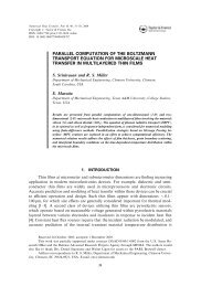
6.1.2. Determining optimal <strong>tolerance</strong><br />
Using <strong>the</strong> closed-form solution defined in Eq. (28), d* becomes<br />
1.0269. This optimal value generates <strong>the</strong> minimum E[TC 2], optimal<br />
LSL, <strong>and</strong> optimal USL at 150.3168, 48.9842, <strong>and</strong> 50.9924, respec-<br />
Table 4<br />
Effect <strong>of</strong> jl Tj on d* when r = r*.<br />
l jl Tj r d* E[CM2] E[CR] E[L2(y)] E[TC2] 49.0 1.00 0.98 0.0685 99.9731 94.5356 5.4726 199.9813<br />
49.1 0.90 0.98 0.4516 99.8230 65.1579 30.4354 195.4162<br />
49.2 0.80 0.98 0.6182 99.7577 53.6425 35.0573 188.4574<br />
49.3 0.70 0.98 0.7345 99.7121 46.2616 34.9641 180.9377<br />
49.4 0.60 0.98 0.8222 99.6777 41.0981 32.8406 173.6164<br />
49.5 0.50 0.98 0.8896 99.6513 37.3676 29.9179 166.9368<br />
49.6 0.40 0.98 0.9412 99.6310 34.6598 26.8931 161.1839<br />
49.7 0.30 0.98 0.9795 99.6160 32.7348 24.1974 156.5482<br />
49.8 0.20 0.98 1.0059 99.6057 31.4458 22.1055 153.1570<br />
49.9 0.10 0.98 1.0215 99.5996 30.7041 20.7882 151.0919<br />
50.0 0.00 0.98 1.0266 99.5976 30.4619 20.3391 150.3987<br />
Fig. 16. Plots <strong>of</strong> <strong>the</strong> effect <strong>of</strong> jl Tj on E[TC2], E[CR], E[L2], E[CM2], <strong>and</strong> d* when<br />
r = r*.<br />
Table 5<br />
Effect <strong>of</strong> r on E[TC 1] when l = l*.<br />
r l E[L1(y)] E[CM1] E[TC1] 0.5 50.00 25.00 307.20 332.20<br />
0.6 50.00 36.00 287.64 323.64<br />
0.7 50.00 49.00 268.08 317.08<br />
0.8 50.00 64.00 248.52 312.52<br />
0.9 50.00 81.00 228.96 309.96<br />
1.0 50.00 100.00 209.40 309.40<br />
1.1 50.00 121.00 189.84 310.84<br />
1.2 50.00 144.00 170.28 314.28<br />
1.3 50.00 169.00 150.72 319.72<br />
1.4 50.00 196.00 131.16 327.16<br />
1.5 50.00 225.00 111.60 336.60<br />
1.6 50.00 256.00 92.04 348.04<br />
1.7 50.00 289.00 72.48 361.48<br />
1.8 50.00 324.00 52.92 376.92<br />
1.9 50.00 361.00 33.36 394.36<br />
2.0 50.00 400.00 13.80 413.80<br />
S. Shin et al. / European Journal <strong>of</strong> Operational Research 207 (2010) 1728–1741 1737<br />
tively. Plots <strong>of</strong> E[TC2], E[CM2], E[CR] <strong>and</strong> E[L2] with respect to d are<br />
presented in Fig. 3.<br />
Figs. 4 <strong>and</strong> 5 show that <strong>the</strong> first derivative <strong>of</strong> E[TC2] with respect<br />
to d at d* is zero <strong>and</strong> <strong>the</strong> second derivative <strong>of</strong> E[TC 2] with respect to<br />
d at d* is greater than zero, respectively. The latter figure also validates<br />
<strong>the</strong> conditions for convexity presented in Eqs. (30) <strong>and</strong> (31).<br />
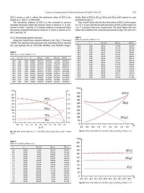
Table 6<br />
Effect <strong>of</strong> l on E[TC 1] when r = r*.<br />
l r E[L1(y)] E[CM1] E[TC1] 49.0 0.98 96.04 210.99 307.03<br />
49.2 0.98 96.04 211.45 307.49<br />
49.4 0.98 96.04 211.92 307.96<br />
49.6 0.98 96.04 212.38 308.42<br />
49.7 0.98 96.04 212.61 308.65<br />
49.8 0.98 96.04 212.85 308.89<br />
49.9 0.98 96.04 213.08 309.12<br />
50.0 0.98 96.04 213.31 309.35<br />
50.1 0.98 96.04 213.54 309.58<br />
50.2 0.98 96.04 213.78 309.82<br />
50.3 0.98 96.04 214.01 310.05<br />
50.4 0.98 96.04 214.24 310.28<br />
50.5 0.98 96.04 214.48 310.52<br />
50.6 0.98 96.04 214.71 310.75<br />
50.8 0.98 96.04 215.17 311.21<br />
51.0 0.98 96.04 215.64 311.68<br />
Fig. 17. Plots <strong>of</strong> <strong>the</strong> effect <strong>of</strong> r on E[TC 1], E[L 1], <strong>and</strong> E[C M1] when l = l*.<br />
Fig. 18. Plots <strong>of</strong> <strong>the</strong> effect <strong>of</strong> l on E[TC 1], E[L 1], <strong>and</strong> E[C M1] when r = r*.