Development of the parametric tolerance modeling and optimization ...
Development of the parametric tolerance modeling and optimization ...
Development of the parametric tolerance modeling and optimization ...

Create successful ePaper yourself
Turn your PDF publications into a flip-book with our unique Google optimized e-Paper software.
1734 S. Shin et al. / European Journal <strong>of</strong> Operational Research 207 (2010) 1728–1741<br />
<strong>and</strong><br />
E½CRŠ ¼CR<br />
Z s d<br />
/ðzÞdz þ<br />
1<br />
Z 1<br />
sþd<br />
/ðzÞdz<br />
¼ CRf1 Uðs þ dÞþUðs dÞg; ð43Þ<br />
where s =(T l*)/r*. Substituting Eqs. (42), (43) <strong>and</strong> (16) into Eq.<br />
(17), <strong>the</strong> expected total cost can be written as<br />
E½TC2Š ¼k ðl TÞ 2 þ r 2<br />
n o<br />
Uðs þ dÞ k ðl TÞ 2 þ r 2<br />
n o<br />
Uðs<br />
k 2r ðl TÞþr<br />
dÞ<br />
2<br />
n o<br />
ðs þ dÞ /ðs þ dÞ<br />
þ k 2r ðl TÞþr 2<br />
n<br />
ðs<br />
o<br />
dÞ /ðs dÞ<br />
þ CRf1 Uðs þ dÞþUðs dÞg þ a0 þ 2a1dr : ð44Þ<br />
Even though <strong>the</strong> closed-form solution <strong>of</strong> d* for this case cannot<br />
be provided, <strong>the</strong> optimum expected total cost <strong>and</strong> d* can be found<br />
by minimizing Eq. (44). After d* is generated, <strong>the</strong> optimal LSL <strong>and</strong><br />
USL can be computed from T d*r* <strong>and</strong> T + d*r*, respectively.<br />
6. Numerical example<br />
To illustrate <strong>the</strong> application <strong>of</strong> <strong>the</strong> proposed models, an electronic<br />
chip manufacturing company experiencing high warranty<br />
costs <strong>and</strong> customer dissatisfaction associated with component failures<br />
in a prime product will be used. This company is considering a<br />
new process for manufacturing electronic chips. In view <strong>of</strong> <strong>the</strong> high<br />
Fig. 2. Plots <strong>of</strong> E[TC1], E[L1], <strong>and</strong>E[CM1] with respect to r <strong>and</strong> l.<br />
Table 1<br />
Effect <strong>of</strong> r on E[TC 1] when l = l*.<br />
r l E[L1(y)] E[CM1] E[TC1] 0.50 49.99 25.01 307.16 332.17<br />
0.60 49.99 36.01 287.60 323.61<br />
0.70 49.99 49.01 268.05 317.06<br />
0.80 49.99 64.01 248.49 312.50<br />
0.90 49.99 81.01 228.93 309.94<br />
1.00 49.99 100.01 209.38 309.39<br />
1.10 49.99 121.01 189.82 310.83<br />
1.20 49.99 144.01 170.27 314.28<br />
1.30 49.99 169.01 150.71 319.72<br />
1.40 49.99 196.01 131.15 327.16<br />
1.50 49.99 225.01 111.60 336.61<br />
1.60 49.99 256.01 92.04 348.05<br />
1.70 49.99 289.01 72.48 361.49<br />
1.80 49.99 324.01 52.93 376.94<br />
1.90 49.99 361.01 33.37 394.38<br />
2.00 49.99 400.01 13.82 413.83<br />
costs associated with <strong>the</strong> failure <strong>of</strong> <strong>the</strong> components <strong>and</strong> <strong>the</strong> low<br />
inspection costs, <strong>the</strong> company follows a 100% inspection policy<br />
on a key quality characteristic Y which is normally distributed with<br />
mean l <strong>and</strong> st<strong>and</strong>ard deviation r.<br />
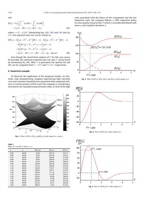
Fig. 3. Plots <strong>of</strong> E[TC2], E[CR], E[L2], <strong>and</strong> E[CM2] with respect to d.<br />
Fig. 4. Plot <strong>of</strong> @E[TC2]/@d with respect to d.<br />
Fig. 5. Plot <strong>of</strong> @ 2 E[TC 2]/@d 2 with respect to d.