Development of the parametric tolerance modeling and optimization ...
Development of the parametric tolerance modeling and optimization ...
Development of the parametric tolerance modeling and optimization ...

You also want an ePaper? Increase the reach of your titles
YUMPU automatically turns print PDFs into web optimized ePapers that Google loves.
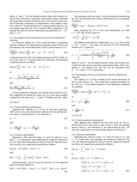
where l*, <strong>and</strong> d 2 , are <strong>the</strong> optimal process mean <strong>and</strong> variance obtained<br />
from <strong>the</strong> process parameter <strong>optimization</strong> phase. Although<br />
<strong>the</strong> closed-from solution presented in Eq. (28) consists <strong>of</strong> <strong>the</strong> Lambert<br />
W function component, its computation is very simple. A negative<br />
value <strong>of</strong> d* is ignored because d is always greater than zero, so<br />
<strong>the</strong> negative sign from Eq. (28) is removed. After computing d*, <strong>the</strong><br />
optimal LSL <strong>and</strong> USL can be respectively calculated from l* d*r*<br />
<strong>and</strong> l* + d*r*.<br />
5.1.3. Investigation <strong>of</strong> <strong>the</strong> second derivative <strong>and</strong> <strong>the</strong> conditions for<br />
convexity<br />
To verify <strong>the</strong> validity <strong>of</strong> d*, <strong>the</strong> second derivative is computed<br />
<strong>and</strong> <strong>the</strong> conditions for obtaining <strong>the</strong> minimum value <strong>of</strong> E[TC2] are<br />
investigated. The second derivative <strong>of</strong> E[TC2] with respect to d is<br />
@ 2 E½TC2Š<br />
@ 2 d<br />
CR 2<br />
¼ 2kd/ðdÞ þ 2r<br />
k<br />
ðl TÞ 2<br />
d 2 r 2<br />
: ð29Þ<br />
d*obtained from Eq. (28) is <strong>the</strong> global minimum <strong>of</strong> E[TC2] if <strong>the</strong> value<br />
<strong>of</strong> Eq. (29) at d* is greater than zero. Therefore, <strong>the</strong> following<br />
conditions must be satisfied:<br />
2kd/ðdÞ CR 2<br />
þ 2r<br />
k<br />
ðl TÞ 2<br />
d 2 r 2 > 0;<br />
or<br />
ffiffiffiffiffiffiffiffiffiffiffiffiffiffiffiffiffiffiffiffiffiffiffiffiffiffiffiffiffiffiffiffiffiffiffiffiffiffiffiffiffiffiffiffiffiffiffiffiffiffiffi<br />
CR þ 2kr<br />
0 < d <<br />
2 kðl TÞ 2<br />
s<br />
; ð30Þ<br />
<strong>and</strong><br />
kr 2<br />
CR þ 2kr 2 kðl TÞ 2<br />
kr 2 > 0: ð31Þ<br />
In many industrial situations, <strong>the</strong> validity <strong>of</strong> this solution is fur<strong>the</strong>r<br />
suggested by setting <strong>the</strong> value <strong>of</strong> CR to a very large number<br />
compared to <strong>the</strong> values <strong>of</strong> l* T <strong>and</strong> r 2 (Phillips <strong>and</strong> Cho, 1998).<br />
5.2. Case II<br />
5.2.1. Process parameter <strong>optimization</strong><br />
Applying <strong>the</strong> condition l = T to Eq. (8) <strong>and</strong> <strong>the</strong>n equating<br />
oE[TC 1]/@r to zero, <strong>the</strong> closed-form solutions for <strong>the</strong> optimal process<br />
mean l* <strong>and</strong> deviation r* are obtained as<br />
l ¼ T; ð32Þ<br />
<strong>and</strong><br />
r ¼ c3l þ c2<br />
2k<br />
or r ¼ c3T þ c2<br />
: ð33Þ<br />
2k<br />
5.2.2. Tolerance <strong>optimization</strong><br />
Replacing l, USL, <strong>and</strong> LSL in Eqs. (11) <strong>and</strong> (13) with T, l + dr,<br />
<strong>and</strong> l dr, respectively, <strong>and</strong> exploiting <strong>the</strong> properties defined in<br />
Eq. (21), <strong>the</strong> expected quality loss E[L 2(y)] <strong>and</strong> <strong>the</strong> expected rejection<br />
cost E[CR] are respectively presented as follows:<br />
E½L2ðyÞŠ ¼ kr 2 ½2UðdÞ 2d/ðdÞ 1Š; ð34Þ<br />
<strong>and</strong><br />
E½CRŠ ¼CR 1<br />
Z d<br />
/ðzÞdz ¼ 2CRf1 UðdÞg: ð35Þ<br />
d<br />
Substituting Eqs. (34), (35) <strong>and</strong> (16) into Eq. (17), <strong>the</strong> expected<br />
total cost can be defined as<br />
E½TC2Š ¼kr 2 f2UðdÞ 2d/ðdÞ 1gþ2CRf1 UðdÞg þ a0 þ 2a1dr :<br />
ð36Þ<br />
S. Shin et al. / European Journal <strong>of</strong> Operational Research 207 (2010) 1728–1741 1733<br />
The minimum total cost <strong>and</strong> d* can be obtained by minimizing<br />
Eq. (36). The first derivative <strong>of</strong> E[TC 2] with respect to d is calculated<br />
as follows:<br />
@E½TC2Š<br />
@d ¼ 2a1r 2CR/ðdÞþ2kd 2 r 2 /ðdÞ: ð37Þ<br />
e 1<br />
2 d2<br />
Then, equating Eq. (37) to zero <strong>and</strong> substituting /(d) with<br />
= ffiffiffiffiffiffi p<br />
2p,<br />
<strong>the</strong> result is given as<br />
kr d 2 CR 1<br />
e 2<br />
kr 2 d2<br />
¼ a1<br />
p : ð38Þ<br />
ffiffiffiffiffiffi<br />
2p<br />
d,<br />
According to Proposition 2, substituting v, g1, g2, g3, <strong>and</strong> g4 with<br />
kr*, CR=kr 2 pffiffiffiffiffiffi , 1/2, <strong>and</strong>a1 2p into Eq. (27), <strong>the</strong> closed-form<br />
solution <strong>of</strong> d* is given by<br />
d ¼<br />
ffiffiffiffiffiffiffiffiffiffiffiffiffiffiffiffiffiffiffiffiffiffiffiffiffiffiffiffiffiffiffiffiffiffiffiffiffiffiffiffiffiffiffiffiffiffiffiffiffiffiffiffiffiffiffiffiffiffiffiffiffiffiffiffiffiffiffiffiffiffiffiffiffiffiffiffiffiffiffiffiffiffiffiffiffiffiffiffiffi<br />
2Lambert W a1<br />
C pffiffiffiffiffiffi<br />
R<br />
2kr 2p e<br />
2<br />
0<br />
1<br />
B<br />
C CR<br />
B<br />
C<br />
@ 2r k A þ<br />
kr 2<br />
v<br />
u<br />
;<br />
t<br />
ð39Þ<br />
where l* <strong>and</strong> r 2 are <strong>the</strong> optimal process mean <strong>and</strong> variance obtained<br />
from <strong>the</strong> process parameter <strong>optimization</strong> phase. After computing<br />
d*, <strong>the</strong> optimal LSL <strong>and</strong> USL can be calculated from<br />
l* d*r* <strong>and</strong> l* + d*r*, respectively.<br />
5.2.3. Investigation <strong>of</strong> <strong>the</strong> second derivative <strong>and</strong> <strong>the</strong> conditions for<br />
convexity<br />
The validity <strong>of</strong> d* can be verified by <strong>the</strong> second derivative <strong>of</strong><br />
E[TC2] with respect to d. The closed-form solution presented in<br />
Eq. (39) <strong>of</strong> d* is <strong>the</strong> global minimum if <strong>the</strong> following conditions<br />
are satisfied:<br />
@ 2 E½TC2Š<br />
@ 2 d<br />
¼ 2kd/ðdÞ CR<br />
k þ 2r 2 ð1 d 2 Þ > 0;<br />
or<br />
ffiffiffiffiffiffiffiffiffiffiffiffiffiffiffiffiffiffiffiffiffi<br />
0 < d < 1 þ CR<br />
r<br />
; ð40Þ<br />
<strong>and</strong><br />
2kr 2<br />
1 þ CR<br />
> 0: ð41Þ<br />
2kr 2<br />
5.3. Case III<br />
5.3.1. Process parameter <strong>optimization</strong><br />
After applying <strong>the</strong> conditions for this case to Eq. (8), <strong>the</strong> expected<br />
total cost is <strong>the</strong> same as that <strong>of</strong> Case I. Thus, <strong>the</strong> optimal<br />
process mean l* <strong>and</strong> deviation r* are determined by Eqs. (19)<br />
<strong>and</strong> (20), respectively. For more details, please see Section 5.1.<br />
5.3.2. Tolerance <strong>optimization</strong><br />
Replacing USL, <strong>and</strong> LSL in Eqs. (11) <strong>and</strong> (13) with T + dr, <strong>and</strong><br />
T dr, respectively, <strong>and</strong> exploiting <strong>the</strong> properties defined in Eq.<br />
(21), <strong>the</strong> expected quality loss E[L2(y)] <strong>and</strong> <strong>the</strong> expected rejection<br />
cost E[CR] are respectively presented as follows:<br />
Z sþd<br />
E½L2ðyÞŠ ¼ kðzr þ l TÞ 2 /ðzÞdz;<br />
or<br />
s d<br />
n o<br />
Uðs þ dÞ<br />
k 2r ðl TÞþr 2<br />
n o<br />
ðs þ dÞ /ðs þ dÞ<br />
k ðl TÞ 2 þ r 2<br />
n o<br />
Uðs dÞ<br />
n o<br />
/ðs dÞ; ð42Þ<br />
E½L2ðyÞŠ ¼ k ðl TÞ 2 þ r 2<br />
þ k 2r ðl TÞþr 2<br />
ðs dÞ