BMJ Statistical Notes Series List by JM Bland: http://www-users.york ...

BMJ Statistical Notes Series 

List by JM Bland: http://www-users.york.ac.uk/~mb55/pubs/pbstnote.htm 

1 Bland JM, Altman DG. Correlation, regression and repeated data. BMJ 1994;308:896 

2 Bland JM, Altman DG. Regression towards the mean. BMJ 1994;308:1499 

3 Altman DG, Bland JM. Diagnostic tests 1: sensitivity and specificity BMJ 1994;308:1552 

4 Altman DG, Bland JM. Diagnostic tests 2: predictive values. BMJ 1994;309:102 

5 Altman DG, Bland JM. Diagnostic tests 3: receiver operating characteristic plots. BMJ 1994;309:188 

6 Bland JM, Altman DG. One- and two-sided tests of significance. BMJ 1994;309:248 

7 Bland JM, Altman DG. Some examples of regression towards the mean. BMJ 1994;309:780 

8 Altman DG, Bland JM. Quartiles, quintliles, centiles, and other quantiles. BMJ 1994;309:996 

9 Bland JM, Altman DG. Matching. BMJ 1994;309:1128 

10 Bland JM, Altman DG. Multiple significance tests: the Bonferroni method. BMJ 1995;310:170 

11 Altman DG, Bland JM. The normal distribution. BMJ 1995;310:298 

12 Bland JM, Altman DG. Calculating correlation coefficients with repeated observations: Part 1, correlation 

within subjects. BMJ 1995;310:446 

13 Bland JM, Altman DG. Calculating correlation coefficients with repeated observations: Part 2, correlation 

between subjects. BMJ 1995;310:633 

14 Altman DG, Bland JM. Absence of evidence is not evidence of absence. BMJ 1995;311:485 

15 Altman DG, Bland JM. Presentation of numerical data. BMJ 1996;312:572 

16 Bland JM, Altman DG. Logarithms. BMJ 1996;312:700 

17 Bland JM, Altman DG. Transforming data. BMJ 1996;312:770 

18 Bland JM, Altman DG. Transformations, means and confidence intervals. BMJ 1996;312:1079 

19 Bland JM, Altman DG. The use of transformations when comparing two means. BMJ 1996;312:1153 

[Dataset bpl 04591] 

20 Altman DG, Bland JM. Comparing several groups using analysis of variance. BMJ 1996;312:1472-1473 

21 Bland JM, Altman DG. Measurement error. BMJ 1996;312:1654 

22 Bland JM, Altman DG. Measurement error and correlation coefficients. BMJ 1996;313:41-42 (includes 

corrected table) 

23 Bland JM, Altman DG. Measurement error proportional to the mean. BMJ 1996;313:106



24 Altman DG, Matthews JNS. Interaction 1: Heterogeneity of effects. BMJ 1996;313:486 

25 Matthews JNS, Altman DG. Interaction 2: compare effect sizes not P values. BMJ 1996;313:808 

26 Matthews JNS, Altman DG. Interaction 3: How to examine heterogeneity. BMJ 1996;313:862 

27 Altman DG, Bland JM. Detecting skewness from summary information. BMJ 1996;313:1200 

28 Bland JM, Altman DG. Cronbach's alpha. BMJ 1997;314:572 

29 Altman DG, Bland JM. Units of analysis. BMJ 1997;314:1874 

30 Bland JM, Kerry SM. Trials randomised in clusters. BMJ 1997;315:600 

31 Kerry SM, Bland JM. Analysis of a trial randomised in clusters. BMJ 1998;316:54 

32 Bland JM, Kerry SM. Weighted comparison of means. BMJ 1998;316:129 

33 Kerry SM, Bland JM. Sample size in cluster randomisation. BMJ 1998;316:549 

34 Kerry SM, Bland JM. The intra-cluster correlation coefficient in cluster randomisation. BMJ 1998;316:1455 

35 Altman DG, Bland JM. Generalisation and extrapolation. BMJ 1998;317:409-410 

36 Altman DG, Bland JM. Time to event (survival) data. BMJ 1998;317:468-469 

37 Bland JM, Altman DG. Bayesians and frequentists BMJ 1998;317:1151 

38 Bland JM, Altman DG. Survival probabilities (the Kaplan-Meier method). BMJ 1998;317:1572 

39 Altman DG, Bland JM. Treatment allocation in controlled trials: why randomise? BMJ 1999;318:1209 

40 Altman DG, Bland JM. Variables and parameters. BMJ 1999;318:1667 

41 Altman DG, Bland JM. How to randomise. BMJ 1999;319:703-704 

42 Bland JM, Altman DG. The odds ratio. BMJ 2000;320:1468 

43 Day SJ, Altman DG. Blinding in clinical trials and other studies. BMJ 2000;321:504 

44 Altman DG, Schulz KF. Concealing treatment allocation in randomised trials. BMJ 2001;323:446-447 

45 Vickers AJ, Altman DG. Analysing controlled trials with baseline and follow up measurements. BMJ 

2001;323:1123-1124 

46 Bland JM, Altman DG. Validating scales and indexes. BMJ 2002;324:606-607 

47 Altman DG, Bland JM. Interaction revisited: the difference between two estimates. BMJ 2003;326:219 

48 Bland JM, Altman DG. The logrank test. BMJ 2004;328:1073



49 Deeks JJ, Altman DG. Diagnostic tests 4: likelihood ratios. BMJ 2004;329:168-169 

50 Altman DG, Bland JM. Treatment allocation by minimisation. BMJ 2005;330:843 

51 Altman DG, Bland JM. Standard deviations and standard errors. BMJ 2005;331:903 

52 Altman DG, Royston P. The cost of dichotomising continuous variables. BMJ 2006;332:1080 

53 Altman DG, Bland JM. Missing data. BMJ 2007;334:424 

54 Altman DG, Bland JM. Parametric v non-parametric methods for data analysis. BMJ 2009;339:170 

55 Bland JM, Altman DG. Analysis of continuous data from small samples. BMJ 2009;339:961-962 

56 Bland JM, Altman DG. Comparisons within randomised groups can be very misleading. BMJ 2011; 342: 

d561 

57 Bland JM, Altman DG. Correlation in restricted ranges of data. BMJ 2011; 343: 577 

58 Altman DG, Bland JM. How to obtain the confidence interval from a P value. BMJ 2011; 343: 681 

59 Altman DG, Bland JM. How to obtain the P value from a confidence interval. BMJ 2011; 343: 682. 

60 Altman DG, Bland JM. Brackets (parentheses) in formulas. BMJ 2011; 343: 578

Downloaded from 

bmj.com on 28 February 2008









































i . ~~ " . 

It 

~, 

I 

; Statistics Notes ' ..,' 

,I ., 

;; , f 

, 

, , ;~ Measurement error 

,.,; r,i 

1; '} 

1 J Martin Bland, Douglas G Altman I 

, ,\ 

j 

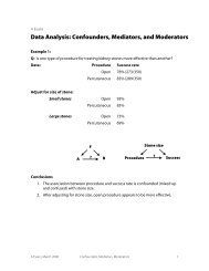
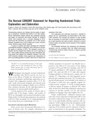
;\ This is the 21st in a series of Several measurements of the same quantity on the same .' 

ij occasional notes on medical subject will not in general be the same. This may be Table 1-Repeated peak ex~/ratory flow rate (PEFR) I 

f measurements for 20 schoolchildren .. 

" stansncs. because of natural vananon m the subject, vananon m ' 

;) ~ shows the measurement four measurements process, of or lung both. function For example, in each table of 20 1 Child PEFR (V mln .) 

1: schoolchildren (taken from a larger study'). The first No 1st 2nd 3rd 4th Mean SO 

I child shows typical variation, having peak expiratory 

! flow rates of 190, 220, 200, and 200 l/min. 1 190 220 200 200 202.50 12.58 ) 

;I' Let us suppose that the child has a "true" average 2 220 200 240 230 222.50 17.08 

! ...3 260 260 240 280 260.00 16.33 

,Ii value over all possIble measurements, which IS what we 4 210 300 280 265 263.75 38.60 

\' really want to know when we make a measurement. 5 270 265 280 270 271.25 6.29 

'" Repeated measurements on the same subject will vary 6 280 280 270 275 276.25 4.79 

j: around the true value because of measurement error. 7 260 280 280 300 280.00 16.33 

i Th ..8 275 275 275 305 282.50 15 00 

, e standard. deVlanon of repeated measure~ents on 9 280 290 300 290 290.00 8:16 

the same subject enables us to measure the sIZe of the 10 320 290 300 290 300.00 14.14 

measurement error. We shall assume that this standard 11 300 300 310 300 302.50 5.00 

deviation is the same for all subjects, as otherwise there 12 270 250 330 370 305.00 55.08 , 

would be no point in estimating it. The main exception 13 320 330 330 330 327.50 5.00 

. h .14 335 320 335 375 341.25 2358 

IS W en the me~surement en:or depends on the sIZe of 15 350 320 340 355 343.75 18:87 

the measurement, usually WIth measurements be com- 16 360 320 350 345 343.75 17.02 

ing more variable as the magnitude of the measurement 17 330 340 380 390 360.00 29.44 

f 60 increases. We deal with this case in a subsequent statis- 18 335 385 360 370 362.50 21.02 

~ ° tics note. The common standard deviation of repeated 19 400 420 425 420 416.25 11.09 

c 20 430 460 480 470 460.00 21.60 

.g measurements IS known as the unthtn-subject standard 

.~ 40 ° deviation, which we shall denote by ~ 

=P: To estimate the within-subject standard deviation, we 

i 20 : .° need several subjects with at least two measurements for standard deviation ~w is given by when n is the number 'j 

~ 0 0 0 ° each. In addition to the data, table 1 also shows the of subjects. We can check for a relation between stand- ' 

.i 0.00 ° mean and standard deviation of the four readings for ard deviation and mean by plotting for each subject the 

~ goo 300 400 500 each child. To get the common within-subject standard absolute value of the difference--that is, ignoring any 

Subject mean (I/min) deviation we actually average the variances, the squares 

FI 1 I d.. d I b. t .of the standard deviations. The mean within-subject 

standard 9 -n deviations IVI ua su plotted !/ec s vanance IS 460.52, so the esumated within-subject 

sign-against the mean. 

The measurement error can be quoted as ~. The 

UliLerence ,... b 

etween a su 

b., 

ject s measurement and the 

against their means standard deviation is ~w= f46o:5 = 21.5 1/min. The true value would be expected to be less than 1. 96 ~w for 

calculation is easier using a program that performs one 95% of observations. Another useful way of presenting 

way analysis ofvariance2 (table 2). The value called the measurement error is sometimes called the repeatability, 

residual mean square is the within-subject variance. which is J2 x 1. 96 ~ or 2. 77~. The difference 

The analysis of variance method is the better approach between two measurements for the same subject is 

in practice, as it deals automatically with the case of expected to be less than 2. 77 ~w for 95% of pairs of 

subjects having different numbers of observations. We observations. For the data in table 1 the repeatability is 

should check the assumption that the standard 2.77 x 2.5 = 60 l/min. The large variability in peak 

deviation is unrelated to the magnitude of the expiratory flow rate is well known, so individual 

measurement. This can be done graphically, by plotting readings of peak expiratory flow are seldom used. 

the individual subject's standard deviations against their The variable used for analysis in the study from which 

means (see fig 1). Any important relation should be table 1 was taken was the mean of the last three 

fairly obvious, but we can check analytically by calculat- readings.' 

.ing a rank correlation coefficient. For the figure there Other ways of describing the repeatability of 

HDePalartm~nt of Public 

S e G th ScIences, ' H .tal 

t eorge s OSpl 

Medical School London 

does not appear to be a relation (Kendall's t = 0.16, 

P - 0 3) 

-..stansncs 

A common design is to take only two measurements 

measurements 

.. 

notes. 

will be considered in subsequent 

SW17 ORE' per subject. In ~s case the method can be simplified I Bland JM, Holland WW, Elliott A. The development of respiratory 

J Martin Bland, professor of because the vanance of two observations is half the symptoms in a cohort of Kent schoolchild~o. Bu/J Physio-~rh Resp 

medical statistics 

IRCF Medical Statistics 

Group, Centre for 

Statistics in Medicine, 

square of their difference. So if the difference between 

th b ..'. ...2 

e two 0 servanons for subject I IS di the WIthin-subject 

1974;10:699-716. 

Altman DG, Bland JM. Comparing several groups using analysis of 

variance. BM] 1996;312:1472. 

. 

Institute of Health Table 2-0ne way analysis of variance for the data of table 1 

Sciences, PO Box 777, 

Oxford OX3 7LF 

0 egrees 0 f Variance .. ratio Probability 

Douglas G Altman, head Source of variation freedom Sum of squares Mean square (F) (P) 

Correspondence to: Children 19 285318.44 15016.78 32.6

" "'.~..~~ ~.v~. a"uu,vu,-~ o'V'-" 'v UCla. u.C VL"~llL'" o.;VI1o.;urr~I11; 

complete destruction of the femoral head. Blood cultures infection. If the diagnosis is missed or delayed, the con- 

grew S auTeUS. His C reactive protein peaked at 122 sequences are serious: the joint destruction may 

mg/!. The hip was drained surgically of large amounts of preclude successful arthroplasty or, perhaps worse, a 

pus, culture of which grew S aureus and Proteus mirabi- hip replacement may be inserted into an unrecognised 

lis. He ~as treated with a prolonged course of high dose septic environment. 

antibiotics, with some clinical improvement but The most userJl non-specific tests seem to be the 

continuing poor mobility. erythrocyte sedimentation rate and measurement of C . 

n an ..~e~ctive ?ro~ein; the single most useful specific test is ~ 

Her DIscussion Jomt asplranon and culture. . 

first These patients were all elderly and had pre-existing We recommend consideration of septic arthritis in 

ng/l. osteoarthritis and concurrent infection elsewhere. any patient with an apparently acute exacerbation of an 

pus None, however, had other systemic conditions predis- osteoarthritic joint, particularly if there is a possibility of 

nar'y posing to infection, such as diabetes, except for the sec- coexistent infection elsewhere. Other possible nonayed 

ond patient, who had a myeloproliferative disorder. The infective causes of a rapid deterioration in symptoms 

,ated development of septic arthritis by haematogenous include pseudogout and avascular necrosis, and these 

was spread was associated with increasing hip pain and will also need to be considered. 

: she rapid destruction of the femoral head. This was accom- Funding: None. 

1 few 

panied by a delay in diagnosis of up to six months. 

Infection in the presence of existing inflammatory 

Conflict ofinterest:None. 

ldio- joint disease, particularly rheumatoid arthritis, is well 

mtis known,' It is much rarer to see this in association with I Gardner GC, Weisman MH. Pyarthrosis in patients with rhewnatoid 

ISIng the much commoner osteoarthrins, although It IS 

arthritis, 

40 years. 

a 

AmJMed 

report of 

1990;88:503-11. 

13 cases and a review of the literature from the past 

ttage 

mm 

recognised! In common with other bone and joint 

. m fi ectlOnS, . th e presentanon . 0 f sepnc . ar thr InS " has 2 Goldenberg DL, Cohen AS. Acute infectious arthritis. Am J Med 

3 Vincent 1976;60:369-77. GM, Amirault )D. Septic arthritis in the elderly. Chn Orthop 

)fhis 

with 

changed in recent years from the usual florid illness. 1991;251:241-5. 

leral 

atec- 

:rred . 

Statistics Notes 

.. 

Measurement error and correlation coefficients 

J Martin Bland, Douglas G Altman 

This is the 22nd in a series of Measurement error is the variation between measure- natural approach when investigating measurement error, 

occasional notes on medical ments of the same quantity on the same individual.! To this will inflate the correlation coefficient, 

statistics quantify measurement error we need repeated measure- The correlation coefficient between repeated measments 

on several subjects. We have discussed the urements is often called the reliability of the 

f within-subject standard deviation as an index of measurement method, It is widely used in the validation 

~ measurement error,! which we like as it has a simple of psychological measures such as scales of anxiety and 

( CliniCal interpretation. Here we consider the use of cor- depression, where it is known as the test-retest reliabilrelation 

coefficients to quantify measurement error, ity,ln such studies it is quoted for different populations 

1 A common design for the investigation of measurement (university students, psychiatric outpatients, etc) 

;teo- " error is to take pairs of measurements on a group of sub- because the correlation coefficient differs between them 

' . I 

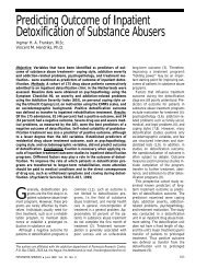
jects, as in table 1. When we have pairs of observations it is as a result of differing ranges of the quantity being 

natural to plot one measurement against the other, The measured, The user has to select the correlation from 

resulting scatter diagram (see figure 1) may tempt us to the study population most like the user's own. 

Departm~nt of Public 

Healtb Sciences, 

S t G ~orge ' s H osp i t al 

calculate a correlation coefficient between the first and 

second measurement. There are difficulties in interpreting 

thi 1 . ffi . In al th 1 . 

between s corre repeated anon coe measurements Clent. gener, will depend e corre on anon the 

Another problem with the use of the correlation coefficient 

between the first and second measurements is 

Table 1-Pairs of measurements of FEV 1 (Htres) a few 

Medical School, London variability between sub'ects. Samples containing subjects weeks apart from 20 Scottish schoolchildren, .tak~n from 

SW17 ORE 

J Martin Bland, professor of 

h 

W 0 

A,a- tl 

UL1Ler grea y 

will J . 

pro duce 1arger corre 1 anon .a larger study (0 Strachan, personal communication) 

medical statistics coefficients than will samples containing similar subjects' 

ICRF M d 1 S ., 

e lca tatlstlcs 

For example, suppose we split 

...easuremen 

this group m whom we have 

measured forced expiratory volume m one second (FEV J 

S b. u Jec 

I 

No 

M 

1 sl 

I 

2nd 

S 

u b. 

No Jec 

Measuremen I 

1 sl 2nd 

Group, Centre for into two subsamples, the first 10 subjects and the second 

Statistics in Medicine, 10 subjects. As table 1 is ordered by the first FEV I 1 1.19 1.37 11 1.54 1.57 

In~titute ofHealtb measurement, both subsamples vary less than does the 2 1.33 1.32 12 1.59 1.60 

ScIences, PO Box 777, 

Oxford OX3 7LF whole sample. 

Th 

e corre 

1 . 

anon 

fi 

or 

th firs 

e 

b 

t su samp 

1 .3 

e IS 4 

1.35 

1.36 

1.40 

1.25 

13 

14 

1.61 

1.61 

1.53 

1.61 

DougiasGAInnanhead r=0.63andfortheseconditisr=0.31,bothlessthan 5 1.36 1.29 15 1.62 1.68 

, r= 0.77 for the full sample. The correlation coefficient 6 1.38 1.37 16 1.78 1.76 

Correspondence to: thus depends on the way the sample is chosen, and it has 7 1.38 1.40 17 1.80 1.82 

Professor Bland. meaning only for the population from which the stUdY: ~::~ ~:~:~: ~:: ~:~~ l 

subjects can be regarded as a random sample. If we select 10 1.431.51 20 2.102.20 l 

EMJ 1996;313:41-2 subjects to give a wide range of the measurement, the Ii 

8M] VOLUME313 6 JULy 1996 41 H 

I 

i 

I 

i

.'.)'. In practice, there will usually be little difference"; 11 

Table 2-0ne way analysis of varianqe for the data in table 1 between r and rI for true repeated measurements. If, 

Source of variation 

Degrees of 

freedom 

Sum of 

squares 

Mean 

square 

Variance 

ratio (F) 

Probability 

(P) 

however, there is a systematic change from the first 

d .gh b db! 

measurement to the secon , as ml t e cause y a 

learning effect, rl will be much less than r. If there was 

"- 

'; 

!' ... 

. 

Children 19 1.52981 0.08052 7.4

Correct data for Statistics Note 

There was an error in Statistics Note 22, Measurement error and correlation coefficients, Bland JM and 

Altman DG, 1996, British Medical Journal 313, 41-2. 

The wrong table of data was printed. The correct data are: 

Sub. 1st 2nd Sub. 1st 2nd 

1 1.20 1.24 11 1.62 1.68 

2 1.21 1.19 12 1.64 1.61 

3 1.42 1.83 13 1.65 2.05 

4 1.43 1.38 14 1.74 1.80 

5 1.49 1.60 15 1.78 1.76 

6 1.58 1.36 16 1.80 1.76 

7 1.58 1.65 17 1.80 1.82 

8 1.59 1.60 18 1.85 1.73 

9 1.60 1.58 19 1.88 1.82 

10 1.61 1.61 20 1.92 2.00

































Statistics notes 

Bayesians and frequentists 

J Martin Bland, Douglas G Altman, 

There are two competing philosophies of statistical 

analysis: the Bayesian and the frequentist. The 

frequentists are much the larger group, and almost all 

the statistical analyses which appear in the BMJ are frequentist. 

The Bayesians are much fewer and until 

recently could only snipe at the frequentists from the 

high ground of university departments of mathematical 

statistics. Now the increasing power of computers is 

bringing Bayesian methods to the fore. 

Bayesian methods are based on the idea that 

unknown quantities, such as population means and 

proportions, have probability distributions. The probability 

distribution for a population proportion 

expresses our prior knowledge or belief about it, before 

we add the knowledge which comes from our data. For 

example, suppose we want to estimate the prevalence 

of diabetes in a health district. We could use the knowledge 

that the percentage of diabetics in the United 

Kingdom as a whole is about 2%, so we expect the 

prevalence in our health district to be fairly similar. It is 

unlikely to be 10%, for example. We might have information 

based on other datasets that such rates vary 

between 1% and 3%, or we might guess that the prevalence 

is somewhere between these values. We can construct 

a prior distribution which summarises our 

beliefs about the prevalence in the absence of specific 

data. We can do this with a distribution having mean 2 

and standard deviation 0.5, so that two standard deviations 

on either side of the mean are 1% and 3%. (The 

precise mathematical form of the prior distribution 

depends on the particular problem.) 

Suppose we now collect some data by a sample 

survey of the district population. We can use the data to 

modify the prior probability distribution to tell us what 

we now think the distribution of the population 

percentage is; this is the posterior distribution. For 

example, if we did a survey of 1000 subjects and found 

15 (1.5%) to be diabetic, the posterior distribution 

would have mean 1.7% and standard deviation 0.3%. 

We can calculate a set of values, a 95% credible interval 

(1.2% to 2.4% for the example), such that there is a 

probability of 0.95 that the percentage of diabetics is 

within this set. The frequentist analysis, which ignores 

the prior information, would give an estimate 1.5% 

with standard error 0.4% and 95% confidence interval 

0.8% to 2.5%. This is similar to the results of the Bayesian 

method, as is usually the case, but the Bayesian 

method gives an estimate nearer the prior mean and a 

narrower interval. 

Frequentist methods regard the population value 

as a fixed, unvarying (but unknown) quantity, without a 

probability distribution. Frequentists then calculate 

confidence intervals for this quantity, or significance 

tests of hypotheses concerning it. Bayesians reasonably 

object that this does not allow us to use our wider 

knowledge of the problem. Also, it does not provide 

what researchers seem to want, which is to be able to 

say that there is a probability of 95% that the 

BMJ VOLUME 317 24 OCTOBER 1998 www.bmj.com 


bmj.com on 28 February 2008 

population value lies within the 95% confidence interval, 

or that the probability that the null hypothesis is 

true is less than 5%. It is argued that researchers want 

this, which is why they persistently misinterpret 

confidence intervals and significance tests in this way. 

A major difficulty, of course, is deciding on the 

prior distribution. This is going to influence the 

conclusions of the study, yet it may be a subjective synthesis 

of the available information, so the same data 

analysed by different investigators could lead to different 

conclusions. Another difficulty is that Bayesian 

methods may lead to intractable computational 

problems. (All widely available statistical packages use 

frequentist methods.) 

Most statisticians have become Bayesians or 

frequentists as a result of their choice of university. 

They did not know that Bayesians and frequentists 

existed until it was too late and the choice had been 

made. There have been subsequent conversions. Some 

who were taught the Bayesian way discovered that 

when they had huge quantities of medical data to analyse 

the frequentist approach was much quicker and 

more practical, although they may remain Bayesian at 

heart. Some frequentists have had Damascus road conversions 

to the Bayesian view. Many practising 

statisticians, however, are fairly ignorant of the 

methods used by the rival camp and too busy to have 

time to find out. 

The advent of very powerful computers has given a 

new impetus to the Bayesians. Computer intensive 

methods of analysis are being developed, which allow 

new approaches to very difficult statistical problems, 

such as the location of geographical clusters of cases of 

a disease. This new practicability of the Bayesian 

approach is leading to a change in the statistical 

paradigm—and a rapprochement between Bayesians 

and frequentists. 12 Frequentists are becoming curious 

about the Bayesian approach and more willing to use 

Bayesian methods when they provide solutions to difficult 

problems. In the future we expect to see more 

Bayesian analyses reported in the BMJ. When this happens 

we may try to use Statistics notes to explain them, 

though we may have to recruit a Bayesian to do it. 

We thank David Spiegelhalter for comments on a draft. 

1 Breslow N. Biostatistics and Bayes (with discussion). Statist Sci 1990;5: 

269-98. 

2 Spiegelhalter DJ, Freedman LS, Parmar MKB. Bayesian approaches to 

randomized trials (with discussion). J R Statist Soc A 1994;157:357-416. 

Correction 

North of England evidence based guidelines development project: 

guideline for the primary care management of dementia 

An editorial error occurred in this article by Martin Eccles 

and colleagues (19 September, pp 802-8). In the list of 

authors the name of Moira Livingston [not Livingstone] was 

misspelt. 

Education and debate 

Department of 

Public Health 

Sciences, St 

George’s Hospital 

Medical School, 

London SW17 0RE 

J Martin Bland, 

professor of medical 

statistics 

ICRF Medical 

Statistics Group, 

Centre for Statistics 

in Medicine, 

Institute of Health 

Sciences, Oxford 

OX3 7LF 

Douglas G Altman, 

head 

Correspondence to: 

Professor Bland 

BMJ 1998;317:1151 

1151

Clinical review 

Department of 

Public Health 

Sciences, St 






statistics 

ICRF Medical 



in Medicine, 



OX3 7LF 


head 




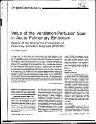
Time (months) to 

conception or 

censoring in 38 

sub-fertile women 

after laparoscopy 

and hydrotubation 2 

Did not 

Conceived conceive 

1 2 

1 3 

1 4 

1 7 

1 7 

1 8 

2 8 

2 9 

2 9 

2 9 

2 11 

3 24 

3 24 

3 

4 

4 

4 

6 

6 

9 

9 

9 

10 

13 

16 




Survival probabilities (the Kaplan-Meier method) 


As we have observed, 1 analysis of survival data requires 

special techniques because some observations are 

censored as the event of interest has not occurred for all 

patients. For example, when patients are recruited over 

two years one recruited at the end of the study may be 

alive at one year follow up, whereas one recruited at the 

start may have died after two years. The patient who died 

has a longer observed survival than the one who still 

survives and whose ultimate survival time is unknown. 

The table shows data from a study of conception in 

subfertile women. 2 The event is conception, and 

women “survived” until they conceived. One woman 

conceived after 16 months (menstrual cycles), whereas 

several were followed for shorter time periods during 

which they did not conceive; their time to conceive was 

thus censored. 

We wish to estimate the proportion surviving (not 

having conceived) by any given time, which is also the 

estimated probability of survival to that time for a 

member of the population from which the sample is 

drawn. Because of the censoring we use the 

Kaplan-Meier method. For each time interval we 

estimate the probability that those who have survived 

to the beginning will survive to the end. This is a conditional 

probability (the probability of being a survivor at 

the end of the interval on condition that the subject 

was a survivor at the beginning of the interval). Survival 

to any time point is calculated as the product of the 

conditional probabilities of surviving each time 

interval. These data are unusual in representing 

months (menstrual cycles); usually the conditional 

probabilities relate to days. The calculations are simplified 

by ignoring times at which there were no recorded 

survival times (whether events or censored times). 

In the example, the probability of surviving for two 

months is the probability of surviving the first month 

times the probability of surviving the second month 

given that the first month was survived. Of 38 women, 

32 survived the first month, or 0.842. Of the 32 women 

at the start of the second month (“at risk” of 

conception), 27 had not conceived by the end of the 

month. The conditional probability of surviving the 

second month is thus 27/32 = 0.844, and the overall 

probability of surviving (not conceiving) after two 

months is 0.842 × 0.844 = 0.711. We continue in this 

way to the end of the table, or until we reach the last 

event. Observations censored at a given time affect the 

number still at risk at the start of the next month. The 

estimated probability changes only in months when 

there is a conception. In practice, a computer is used to 

do these calculations. Standard errors and confidence 

intervals for the estimated survival probabilities can be 

found by Greenwood’s method. 3 Survival probabilities 

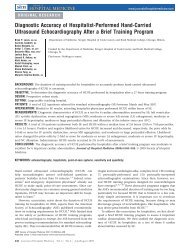
are usually presented as a survival curve (figure). The 

“curve” is a step function, with sudden changes in the 

estimated probability corresponding to times at which 

an event was observed. The times of the censored data 

are indicated by short vertical lines. 

Survival probability 

1.0 

0.75 

0.5 

0.25 

0 

0 6 12 18 24 

Time (months) 

Survival curve showing probability of not conceiving among 38 

subfertile women after laparoscopy and hydrotubation 2 

There are three assumptions in the above. Firstly, 

we assume that at any time patients who are censored 

have the same survival prospects as those who 

continue to be followed. This assumption is not easily 

testable. Censoring may be for various reasons. In the 

conception study some women had received hormone 

treatment to promote ovulation, and others had 

stopped trying to conceive. Thus they were no longer 

part of the population we wanted to study, and their 

survival times were censored. In most studies some 

subjects drop out for reasons unrelated to the 

condition under study (for example, emigration) If, 

however, for some patients in this study censoring was 

related to failure to conceive this would have biased the 

estimated survival probabilities downwards. 

Secondly, we assume that the survival probabilities 

are the same for subjects recruited early and late in the 

study. In a long term observational study of patients 

with cancer, for example, the case mix may change over 

the period of recruitment, or there may be an innovation 

in ancillary treatment. This assumption may be 

tested, provided we have enough data to estimate 

survival curves for different subsets of the data. 

Thirdly, we assume that the event happens at the 

time specified. This is not a problem for the conception 

data, but could be, for example, if the event were recurrence 

of a tumour which would be detected at a regular 

examination. All we would know is that the event 

happened between two examinations. This imprecision 

would bias the survival probabilities upwards. When 

the observations are at regular intervals this can be 

allowed for quite easily, using the actuarial method. 3 

Formal methods are needed for testing hypotheses 

about survival in two or more groups. We shall describe 

the logrank test for comparing curves and the more 

complex Cox regression model in future Notes. 

1 Altman DG, Bland JM. Time to event (survival) data. BMJ 

1997;317:468-9. 

2 Luthra P, Bland JM, Stanton SL. Incidence of pregnancy after 

laparoscopy and hydrotubation. BMJ 1982;284:1013-4. 

3 Parmar MKB, Machin D. Survival analysis: a practical approach. Chichester: 

Wiley, 37, 47-9. 

1572 BMJ VOLUME 317 5 DECEMBER 1998 www.bmj.com


Treatment allocation in controlled trials: why randomise? 

Douglas G Altman, J Martin Bland 

Since 1991 the BMJ has had a policy of not publishing 

trials that have not been properly randomised, except 

in rare cases where this can be justified. 1 Why? 

The simplest approach to evaluating a new 

treatment is to compare a single group of patients 

given the new treatment with a group previously 

treated with an alternative treatment. Usually such 

studies compare two consecutive series of patients in 

the same hospital(s). This approach is seriously flawed. 

Problems will arise from the mixture of retrospective 

and prospective studies, and we can never satisfactorily 

eliminate possible biases due to other factors (apart 

from treatment) that may have changed over time. 

Sacks et al compared trials of the same treatments in 

which randomised or historical controls were used and 

found a consistent tendency for historically controlled 

trials to yield more optimistic results than randomised 

trials. 2 The use of historical controls can be justified 

only in tightly controlled situations of relatively rare 

conditions, such as in evaluating treatments for 

advanced cancer. 

The need for contemporary controls is clear, but 

there are difficulties. If the clinician chooses which 

treatment to give each patient there will probably be 

differences in the clinical and demographic characteristics 

of the patients receiving the different treatments. 

Much the same will happen if patients choose their 

own treatment or if those who agree to have a 

treatment are compared with refusers. Similar problems 

arise when the different treatment groups are at 

different hospitals or under different consultants. Such 

systematic differences, termed bias, will lead to an overestimate 

or underestimate of the difference between 

treatments. Bias can be avoided by using random allocation. 

A well known example of the confusion engendered 

by a non-randomised study was the study of the 

possible benefit of vitamin supplementation at the time 

of conception in women at high risk of having a baby 

with a neural tube defect. 3 The investigators found that 

the vitamin group subsequently had fewer babies with 

neural tube defects than the placebo control group. 

The control group included women ineligible for the 

trial as well as women who refused to participate. As a 

consequence the findings were not widely accepted, 

and the Medical Research Council later funded a large 

randomised trial to answer to the question in a way that 

would be widely accepted. 4 

The main reason for using randomisation to 

allocate treatments to patients in a controlled trial is to 

prevent biases of the types described above. We want to 

compare the outcomes of treatments given to groups 

of patients which do not differ in any systematic way. 

Another reason for randomising is that statistical 

theory is based on the idea of random sampling. In a 

study with random allocation the differences between 

treatment groups behave like the differences between 

random samples from a single population. We know 

BMJ VOLUME 318 1 MAY 1999 www.bmj.com 



how random samples are expected to behave and so 

can compare the observations with what we would 

expect if the treatments were equally effective. 

The term random does not mean the same as haphazard 

but has a precise technical meaning. By random 

allocation we mean that each patient has a known 

chance, usually an equal chance, of being given each 

treatment, but the treatment to be given cannot be predicted. 

If there are two treatments the simplest method 

of random allocation gives each patient an equal 

chance of getting either treatment; it is equivalent to 

tossing a coin. In practice most people use either a 

table of random numbers or a random number 

generator on a computer. This is simple randomisation. 

Possible modifications include block randomisation, 

to ensure closely similar numbers of patients in 

each group, and stratified randomisation, to keep the 

groups balanced for certain prognostic patient characteristics. 

We discuss these extensions in a subsequent 

Statistics note. 

Fifty years after the publication of the first 

randomised trial 5 the technical meaning of the term 

randomisation continues to elude some investigators. 

Journals continue to publish “randomised” trials which 

are no such thing. One common approach is to 

allocate treatments according to the patient’s date of 

birth or date of enrolment in the trial (such as giving 

one treatment to those with even dates and the other to 

those with odd dates), by the terminal digit of the hospital 

number, or simply alternately into the different 

treatment groups. While all of these approaches are in 

principle unbiased—being unrelated to patient 

characteristics—problems arise from the openness of 

the allocation system. 1 Because the treatment is known 

when a patient is considered for entry into the trial this 

knowledge may influence the decision to recruit that 

patient and so produce treatment groups which are 

not comparable. 

Of course, situations exist where randomisation is 

simply not possible. 6 The goal here should be to retain 

all the methodological features of a well conducted 

randomised trial 7 other than the randomisation. 

1 Altman DG. Randomisation. BMJ 1991;302:1481-2. 

2 Sacks H, Chalmers TC, Smith H. Randomized versus historical controls 

for clinical trials. Am J Med 1982;72:233-40. 

3 Smithells RW, Sheppard S, Schorah CJ, Seller MJ, Nevin NC, Harris R, et 

al. Possible prevention of neural-tube defects by periconceptional vitamin 

supplementation. Lancet 1980;i:339-40. 

4 MRC Vitamin Study Research Group. Prevention of neural tube defects: 

results of the Medical Research Council vitamin study. Lancet 

1991;338:131-7. 

5 Medical Research Council. Streptomycin treatment of pulmonary tuberculosis. 

BMJ 1948;2:769-82. 

6 Black N. Why we need observational studies to evaluate the effectiveness 

of health care. BMJ 1996;312:1215-8. 

7 Begg C, Cho M, Eastwood S, Horton R, Moher D, Olkin I, et al. Improving 

the quality of reporting of randomized controlled trials: the 

CONSORT Statement. JAMA 1996;276:637-9. 


ICRF Medical 



in Medicine, 



OX3 7LF 


professor of statistics 

in medicine 

Department of 

Public Health 

Sciences, St 






statistics 


Professor Altman. 


1209

15 Van den Hoogen HJM, Koes BW, van Eijk JT, Bouter LM, Devillé W. On 

the course of low back pain in general practice: a one year follow up 

study. Ann Rheum Dis 1998;57:13-9. 

16 Croft PR, Papageorgiou AC, Ferry S, Thomas E, Jayson MIV, Silman AJ. 

Psychological distress and low back pain: Evidence from a prospective 

study in the general population. Spine 1996;20:2731-7. 

17 Papageorgiou AC, Macfarlane GJ, Thomas E, Croft PR, Jayson MIV, 

Silman AJ. Psychosocial factors in the work place—do they predict new 

episodes of low back pain? Spine 1997;22:1137-42. 

18 Main CJ, Wood PL, Hollis S, Spanswick CC, Waddell G. The distress and 

risk assessment method. A simple patient classification to identify distress 

and evaluate the risk of poor outcome. Spine 1992;17:42-52. 

19 Coste J, Delecoeuillerie G, Cohen de Lara A, Le Parc JM, Paolaggi JB. 

Clinical course and prognostic factors in acute low back pain: an inception 

cohort study in primary care practice. BMJ 1994;308:577-80. 


Variables and parameters 


Like all specialist areas, statistics has developed its own 

language. As we have noted before, 1 much confusion 

may arise when a word in common use is also given a 

technical meaning. Statistics abounds in such terms, 

including normal, random, variance, significant, etc. 

Two commonly confused terms are variable and 

parameter; here we explain and contrast them. 

Information recorded about a sample of individuals 

(often patients) comprises measurements such as 

blood pressure, age, or weight and attributes such as 

blood group, stage of disease, and diabetes. Values of 

these will vary among the subjects; in this context 

blood pressure, weight, blood group and so on are 

variables. Variables are quantities which vary from 

individual to individual. 

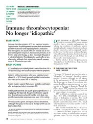
By contrast, parameters do not relate to actual 

measurements or attributes but to quantities defining a 

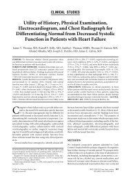
theoretical model. The figure shows the distribution of 

measurements of serum albumin in 481 white men 

aged over 20 with mean 46.14 and standard deviation 

3.08 g/l. For the empirical data the mean and SD are 

called sample estimates. They are properties of the collection 

of individuals. Also shown is the normal 1 distribution 

which fits the data most closely. It too has mean 

46.14 and SD 3.08 g/l. For the theoretical distribution 

the mean and SD are called parameters. There is not 

one normal distribution but many, called a family of 

distributions. Each member of the family is defined by 

its mean and SD, the parameters 1 which specify the 

particular theoretical normal distribution with which 

we are dealing. In this case, they give the best estimate 

of the population distribution of serum albumin if we 

can assume that in the population serum albumin has 

a normal distribution. 

Most statistical methods, such as t tests, are called 

parametric because they estimate parameters of some 

underlying theoretical distribution. Non-parametric 

methods, such as the Mann-Whitney U test and the log 

rank test for survival data, do not assume any particular 

family for the distribution of the data and so do not 

estimate any parameters for such a distribution. 

Another use of the word parameter relates to its 

original mathematical meaning as the value(s) defining 

one of a family of curves. If we fit a regression model, 

such as that describing the relation between lung function 

and height, the slope and intercept of this line 

BMJ VOLUME 318 19 JUNE 1999 www.bmj.com 



20 Dionne CE, Koepsell TD, Von Korff M, Deyo RA, Barlow WE, Checkoway 

H. Predicting long-term functional limitations among back pain patients 

in primary care. J Clin Epidemiol 1997;50:31-43. 

21 Macfarlane GJ, Thomas E, Papageorgiou AC, Schollum J, Croft PR. The 

natural history of chronic pain in the community: a better prognosis than 

in the clinic? J Rheumatol 1996;23:1617-20. 

22 Troup JDG, Martin JW, Lloyd DCEF. Back pain in industry. A prospective 

survey. Spine 1981;6:61-9. 

23 Burton AK, Tillotson KM. Prediction of the clinical course of low-back 

trouble using multivariable models. Spine 1991;16:7-14. 

24 Pope MH, Rosen JC, Wilder DG, Frymoyer JW. The relation between biomechanical 

and psychological factors in patients with low-back pain. 

Spine 1980;5:173-8. 

Frequency 

(Accepted 31 March 1999) 

80 

60 

40 

20 

0 

35 40 45 50 55 

Albumin (g/l) 

Measurements of serum albumin in 481 white men aged over 20 

(data from Dr W G Miller) 

(more generally known as regression coefficients) are 

the parameters defining the model. They have no 

meaning for individuals, although they can be used to 

predict an individual’s lung function from their height. 

In some contexts parameters are values that can be 

altered to see what happens to the performance of 

some system. For example, the performance of a 

screening programme (such as positive predictive 

value or cost effectiveness) will depend on aspects such 

as the sensitivity and specificity of the screening test. If 

we look to see how the performance would change if, 

say, sensitivity and specificity were improved, then we 

are treating these as parameters rather than using the 

values observed in a real set of data. 

Parameter is a technical term which has only 

recently found its way into general use, unfortunately 

without keeping its correct meaning. It is common in 

medical journals to find variables incorrectly called 

parameters (but not in the BMJ we hope 2 ). Another 

common misuse of parameter is as a limit or boundary, 

as in “within certain parameters.” This misuse seems to 

have arisen from confusion between parameter and 

perimeter. 

Misuse of medical terms is rightly deprecated. Like 

other language errors it leads to confusion and the loss 

of valuable distinction. Misuse of non-medical terms 

should be viewed likewise. 

1 Altman DG, Bland JM. The normal distribution. BMJ 1995;310:298. 

2 Endpiece: What’s a parameter? BMJ 1998;316:1877. 

General practice 

ICRF Medical 



in Medicine, 



OX3 7LF 



in medicine 

Department of 

Public Health 

Sciences, St 






statistics 




1667

Much work still needs to be done to achieve this. To be 

useful in health policy at this level, all the targets need 

to be elaborated further and clear, practical statements 

must be made on their operation—especially the four 

targets on health policy and sustainable health systems. 

The WHO should stimulate the discussion of these 

important targets, but it should also be careful about 

being too prescriptive about health systems since this 

could be counterproductive. 

In addition, more attention should be given to the 

usefulness of the targets in member states. One way of 

doing this is to rank the countries by target and to 

divide them into three groups. A specific level could be 

set for each group. For example, for target 2, three such 

groups could be distinguished as follows: 

x Countries that have already achieved this target 

x Countries for which the global target is achievable 

and challenging 

x Countries that find the global target hard to achieve 

and therefore “demotivating.” 

The first group needs stricter target levels, and the 

third group less stringent ones. If a breakdown of this 

kind is made for each target, some countries may be 

classified in different groups for different targets. In this 

way, the targets will provide an insight into the health 

status of the population and could be useful for policy 

makers in member states in encouraging action and 

allocating their resources. 

We thank Dr J Visschedijk and Professor L J Gunning-Schepers 

and other referees of this article for their helpful comments. 

Funding: This study was commissioned by Policy Action 

Coordination at the WHO and supported by an unrestricted 

educational grant from Merck & Co Inc, New Jersey, USA. 

Competing interests: None declared. 

1 World Health Assembly. Resolution WHA51.7. Health for all policy for the 

twenty-first century. Geneva: World Health Organisation, 1998. 

2 World Health Association. Health for all in the 21st century. Geneva: WHO, 

1998. 


How to randomise 


We have explained why random allocation of 

treatments is a required feature of controlled trials. 1 

Here we consider how to generate a random allocation 

sequence. 

Almost always patients enter a trial in sequence 

over a prolonged period. In the simplest procedure, 

simple randomisation, we determine each patient’s 

treatment at random independently with no constraints. 

With equal allocation to two treatment groups 

this is equivalent to tossing a coin, although in practice 

coins are rarely used. Instead we use computer generated 

random numbers. Suitable tables can be found in 

most statistics textbooks. The table shows an example 2 : 

the numbers can be considered as either random digits 

from 0 to 9 or random integers from 0 to 99. 

For equal allocation to two treatments we could 

take odd and even numbers to indicate treatments A 

and B respectively. We must then choose an arbitrary 

BMJ VOLUME 319 11 SEPTEMBER 1999 www.bmj.com 



3 World Health Association. Global strategy for health for all by the year 2000. 

Geneva: WHO, 1981. (WHO Health for All series No 3.) 

4 Visschedijk J, Siméant S. Targets for health for all in the 21st century. 

World Health Stat Q 1998;51:56-67. 

5 Van de Water HPA, van Herten LM. Never change a winning team? Review 

of WHO’s new global policy: health for all in the 21st century. Leiden: TNO 

Prevention and Health, 1999. 

6 World Health Organisation. Bridging the gaps. Geneva: WHO, 1995. 

(World health report.) 

7 World Health Organisation. Fighting disease, fostering development. Geneva: 

WHO, 1996. (World health report.) 

8 World Health Organisation. 1997: Conquering suffering,enriching humanity. 

Geneva: WHO, 1997. (World health report.) 

9 Murray CJL, Lopez AD, eds. The global burden of disease. Boston: Harvard 

University Press, 1996. 

10 United Nations. The world population prospects. New York: UN, 1998. 

11 United Nations Development Programme. Human development report 

1997. New York: Oxford University Press, 1997. 

12 World Bank. Poverty reduction and the World Bank: progress and challenges in 

the 1990s. New York: World Bank, 1996. 

13 World Health Organisation. Third evaluation of health for all by the year 

2000. Geneva: WHO, 1999. (In press.) 

14 Ad Hoc Committee on Health Research Relating to Future Intervention 

Options. Investing in health research and development. Geneva: WHO,1996. 

(Document TDR/Gen/96.1.) 

15 Taylor CE. Surveillance for equity in primary health care: policy implications 

from international experience. Int J Epidemiol 1992;21:1043-9. 

16 Frerichs RR. Epidemiologic surveillance in developing countries. Annu 

Rev Public Health 1991;12:257-80. 

17 World Health Organisation. Health for all renewal—building sustainable 

health systems: from policy to action. Report of meeting on 17-19 November 1997 

in Helsinki, Finland. Geneva: WHO, 1998. 

18 World Health Organisation. EMC annual report 1996. Geneva: WHO: 

1996. 

19 World Health Organisation. Physical status: the use and interpretation of 

anthropometry of a WHO expert committee. Geneva: WHO, 1995. (WHO 

technical report series No 834.) 

20 World Health Organisation. Global database on child growth and malnutrition. 

Geneva: WHO, 1997. 

21 World Health Organisation. Tobacco or health:a global status report. Geneva: 

WHO, 1997. 

22 Erkens C. Cost-effectiveness of ‘short course chemotherapy’ in smear-negative 

tuberculosis. Utrecht: Netherlands School of Public Health, 1996. 

23 Van de Water HPA, van Herten LM. Bull’s eye or Achilles’ heel: WHO’s European 

health for all targets evaluated in the Netherlands. Leiden: Netherlands 

Association for Applied Scientific Research (TNO) Prevention and 

Health, 1996. 

24 Van de Water HPA, van Herten LM. Health policies on target? Review of 

health target and priority setting in 18 European countries. Leiden: 

Netherlands Association for Applied Scientific Research (TNO) Prevention 

and Health, 1998. 

(Accepted 4 May 1999) 

place to start and also the direction in which to read 

the table. The first 10 two digit numbers from a starting 

place in column 2 are 85 80 62 36 96 56 17 17 23 87, 

which translate into the sequence ABBBBBAAA 

A for the first 10 patients. We could instead have taken 

each digit on its own, or numbers 00 to 49 for A and 50 

to 99 for B. There are countless possible strategies; it 

makes no difference which is used. 

We can easily generalise the approach. With three 

groups we could use 01 to 33 for A, 34 to 66 for B, and 

67 to 99 for C (00 is ignored). We could allocate treatments 

A and B in proportions 2 to 1 by using 01 to 66 

for A and 67 to 99 for B. 

At any point in the sequence the numbers of 

patients allocated to each treatment will probably 

differ, as in the above example. But sometimes we want 

to keep the numbers in each group very close at all 

times. Block randomisation (also called restricted 


ICRF Medical 



in Medicine, 



OX3 7LF 



in medicine 

Department of 

Public Health 

Sciences, St 






statistics 



BMJ 1999;319:703–4 

703


Excerpt from a table of random digits. 2 The numbers used in the 

example are shown in bold 

89 11 77 99 94 

35 83 73 68 20 

84 85 95 45 52 

56 80 93 52 82 

97 62 98 71 39 

79 36 13 72 99 

34 96 98 54 89 

69 56 88 97 43 

09 17 78 78 02 

83 17 39 84 16 

24 23 36 44 14 

39 87 30 20 41 

75 18 53 77 83 

33 93 39 24 81 

22 52 01 86 71 

randomisation) is used for this purpose. For example, if 

we consider subjects in blocks of four at a time there 

are only six ways in which two get A and two get B: 

1:AABB2:ABAB3:ABBA4:BBAA5:BA 

BA6:BAAB 

We choose blocks at random to create the 

allocation sequence. Using the single digits of the previous 

random sequence and omitting numbers outside 

the range 1 to 6 we get 5623665611.From these 

we can construct the block allocation sequence BAB 

A/BAAB/ABAB/ABBA/BAAB,andsoon. 

The numbers in the two groups at any time can never 

differ by more than half the block length. Block size is 

normally a multiple of the number of treatments. 

Large blocks are best avoided as they control balance 

less well. It is possible to vary the block length, again at 

random, perhaps using a mixture of blocks of size 2, 4, 

or 6. 

While simple randomisation removes bias from the 

allocation procedure, it does not guarantee, for example, 

that the individuals in each group have a similar 

age distribution. In small studies especially some 

chance imbalance will probably occur, which might 

complicate the interpretation of results. We can use 

stratified randomisation to achieve approximate 

balance of important characteristics without sacrificing 

the advantages of randomisation. The method is to 

produce a separate block randomisation list for each 

subgroup (stratum). For example, in a study to 

One hundred years ago 

Generalisation of salt infusions 

The subcutaneous infusion of salt solution has proved of great 

benefit in the treatment of collapse after severe operations. The 

practice, it may be said, developed from two sources: the new 

method of transfusion where water, instead of another person’s 

blood, is injected into the patient’s veins; and flushing of the 

peritoneum, introduced by Lawson Tait. After flushing, much of 

the fluid left in the peritoneum is absorbed into the circulation, 

greatly to the patient’s advantage. Dr. Clement Penrose has tried 

the effect of subcutaneous salt infusions as a last extremity in 

severe cases of pneumonia. He continues this treatment with 

inhalations of oxygen. He has had experience of three cases, all 

considered hopeless, and succeeded in saving one. In the other 

two the prolongation of life and the relief of symptoms were so 

marked that Dr. Penrose regretted that the treatment had not 



compare two alternative treatments for breast cancer it 

might be important to stratify by menopausal status. 

Separate lists of random numbers should then be constructed 

for premenopausal and postmenopausal 

women. It is essential that stratified treatment 

allocation is based on block randomisation within each 

stratum rather than simple randomisation; otherwise 

there will be no control of balance of treatments within 

strata, so the object of stratification will be defeated. 

Stratified randomisation can be extended to two or 

more stratifying variables. For example, we might want 

to extend the stratification in the breast cancer trial to 

tumour size and number of positive nodes. A separate 

randomisation list is needed for each combination of 

categories. If we had two tumour size groups (say 4cm) and three groups for node involvement (0, 

1-4, > 4) as well as menopausal status, then we have 

2 × 3 × 2 = 12 strata, which may exceed the limit of what 

is practical. Also with multiple strata some of the combinations 

of categories may be rare, so the intended 

treatment balance is not achieved. 

In a multicentre study the patients within each centre 

will need to be randomised separately unless there 

is a central coordinated randomising service. Thus 

“centre” is a stratifying variable, and there may be other 

stratifying variables as well. 

In small studies it is not practical to stratify on more 

than one or perhaps two variables, as the number of 

strata can quickly approach the number of subjects. 

When it is really important to achieve close similarity 

between treatment groups for several variables 

minimisation can be used—we discuss this method in a 

separate Statistics note. 3 

We have described the generation of a random 

sequence in some detail so that the principles are clear. 

In practice, for many trials the process will be done by 

computer. Suitable software is available at http:// 

www.sghms.ac.uk/phs/staff/jmb/jmb.htm. 

We shall also consider in a subsequent note the 

practicalities of using a random sequence to allocate 

treatments to patients. 

1 Altman DG, Bland JM. Treatment allocation in controlled trials: why randomise? 

BMJ 1999;318:1209. 

2 Altman DG. Practical statistics for medical research. London: Chapman and 

Hall, 1990: 540-4. 

3 Treasure T, MacRae KD. Minimisation: the platinum standard for trials? 


been employed earlier. Several physicians have adopted Dr. 

Penrose’s method, and with the most gratifying results. The cases 

are reported fully in the Bulletin of the Johns Hopkins Hospital for 

July last. The infusions of salt solution were administered just as 

after an operation. The salt solution, at a little above body 

temperature, is poured into a graduated bottle connected by a 

rubber tube with a needle. The pressure is regulated by elevating 

the bottle, or by means of a rubber bulb with valves; the needle is 

introduced into the connective tissue under the breast or under 

the integuments of the thighs. There can be no doubt that 

subcutaneous saline infusions are increasing in popularity, and 

little doubt that their use will be greatly extended in medicine as 

well as surgery. 

(BMJ 1899;ii:933) 

704 BMJ VOLUME 319 11 SEPTEMBER 1999 www.bmj.com


Department of 

Public Health 

Sciences, 

St George’s 

Hospital Medical 

School, London 

SW17 0RE 

J Martin Bland 


statistics 

ICRF Medical 



in Medicine, 



OX3 7LF 

Douglas G Altman 


in medicine 





The odds ratio 




In recent years odds ratios have become widely used in 

medical reports—almost certainly some will appear in 

today’s BMJ. There are three reasons for this. Firstly, 

they provide an estimate (with confidence interval) for 

the relationship between two binary (“yes or no”) variables. 

Secondly, they enable us to examine the effects of 

other variables on that relationship, using logistic 

regression. Thirdly, they have a special and very 

convenient interpretation in case-control studies (dealt 

with in a future note). 

The odds are a way of representing probability, 

especially familiar for betting. For example, the odds 

that a single throw of a die will produce a six are 1 to 

5, or 1/5. The odds is the ratio of the probability that 

the event of interest occurs to the probability that it 

does not. This is often estimated by the ratio of the 

number of times that the event of interest occurs to 

the number of times that it does not. The table shows 

data from a cross sectional study showing the 

prevalence of hay fever and eczema in 11 year old 

children. 1 The probability that a child with eczema will 

also have hay fever is estimated by the proportion 

141/561 (25.1%). The odds is estimated by 141/420. 

Similarly, for children without eczema the probability 

of having hay fever is estimated by 928/14 453 (6.4%) 

and the odds is 928/13 525. We can compare the 

groups in several ways: by the difference between the 

proportions, 141/561 − 928/14 453 = 0.187 (or 18.7 

percentage points); the ratio of the proportions, (141/ 

561)/(928/14 453) = 3.91 (also called the relative 

risk); or the odds ratio, (141/420)/(928/ 

13 525) = 4.89. 

Association between hay fever and eczema in 11 year old 

children 1 

Hay fever 

Eczema 

Yes No 

Total 

Yes 141 420 561 

No 928 13 525 14 453 

Total 1069 13 945 15 522 

Now, suppose we look at the table the other way 

round, and ask what is the probability that a child with 

hay fever will also have eczema? The proportion is 

141/1069 (13.2%) and the odds is 141/928. For a 

child without hay fever, the proportion with eczema is 

420/13 945 (3.0%) and the odds is 420/13 525. Comparing 

the proportions this way, the difference is 141/ 

1069 − 420/13 945 = 0.102 (or 10.2 percentage 

points); the ratio (relative risk) is (141/1069)/(420/ 

13 945) = 4.38; and the odds ratio is (141/928)/(420/ 

13 525) = 4.89. The odds ratio is the same whichever 

way round we look at the table, but the difference and 

ratio of proportions are not. It is easy to see why this is. 

The two odds ratios are 

which can both be rearranged to give 

If we switch the order of the categories in the rows and 

the columns, we get the same odds ratio. If we switch 

the order for the rows only or for the columns only, we 

get the reciprocal of the odds ratio, 1/4.89 = 0.204. 

These properties make the odds ratio a useful 

indicator of the strength of the relationship. 

The sample odds ratio is limited at the lower end, 

since it cannot be negative, but not at the upper end, 

and so has a skew distribution. The log odds ratio, 2 

however, can take any value and has an approximately 

Normal distribution. It also has the useful property that 

if we reverse the order of the categories for one of the 

variables, we simply reverse the sign of the log odds 

ratio: log(4.89) = 1.59, log(0.204) = − 1.59. 

We can calculate a standard error for the log odds 

ratio and hence a confidence interval. The standard 

error of the log odds ratio is estimated simply by the 

square root of the sum of the reciprocals of the four 

frequencies. For the example, 

A 95% confidence interval for the log odds ratio is 

obtained as 1.96 standard errors on either side of the 

estimate. For the example, the log odds ratio is 

log e(4.89) = 1.588 and the confidence interval is 

1.588±1.96×0.103, which gives 1.386 to 1.790. We can 

antilog these limits to give a 95% confidence interval 

for the odds ratio itself, 2 as exp(1.386) = 4.00 to 

exp(1.790) = 5.99. The observed odds ratio, 4.89, is not 

in the centre of the confidence interval because of the 

asymmetrical nature of the odds ratio scale. For this 

reason, in graphs odds ratios are often plotted using a 

logarithmic scale. The odds ratio is 1 when there is no 

relationship. We can test the null hypothesis that the 

odds ratio is 1 by the usual 2 test for a two by two 

table. 

Despite their usefulness, odds ratios can cause difficulties 

in interpretation. 3 We shall review this debate 

and also discuss odds ratios in logistic regression and 

case-control studies in future Statistics Notes. 

We thank Barbara Butland for providing the data. 

1 Strachan DP, Butland BK, Anderson HR. Incidence and prognosis of 

asthma and wheezing illness from early childhood to age 33 in a national 

British cohort. BMJ. 1996;312:1195-9. 

2 Bland JM, Altman DG. Transforming data. BMJ 1996;312:770. 

3 Sackett DL, Deeks JJ, Altman DG. Down with odds ratios! Evidence-Based 

Med 1996;1:164-6. 

1468 BMJ VOLUME 320 27 MAY 2000 bmj.com


Leo 

Pharmaceuticals, 

Princes Risborough, 

Buckinghamshire 

HP27 9RR 

Simon J Day 

manager, clinical 

biometrics 

ICRF Medical 




OX3 7LF 



in medicine 


SJDay 



Blinding in clinical trials and other studies 

Simon J Day, Douglas G Altman 



Human behaviour is influenced by what we know or 

believe. In research there is a particular risk of expectation 

influencing findings, most obviously when there is 

some subjectivity in assessment, leading to biased 

results. Blinding (sometimes called masking) is used to 

try to eliminate such bias. 

It is a tenet of randomised controlled trials that the 

treatment allocation for each patient is not revealed 

until the patient has irrevocably been entered into the 

trial, to avoid selection bias. This sort of blinding, better 

referred to as allocation concealment, will be discussed 

in a future statistics note. In controlled trials the term 

blinding, and in particular “double blind,” usually 

refers to keeping study participants, those involved 

with their management, and those collecting and analysing 

clinical data unaware of the assigned treatment, 

so that they should not be influenced by that 

knowledge. 

The relevance of blinding will vary according to 

circumstances. Blinding patients to the treatment they 

have received in a controlled trial is particularly important 

when the response criteria are subjective, such as 

alleviation of pain, but less important for objective criteria, 

such as death. Similarly, medical staff caring for 

patients in a randomised trial should be blinded to 

treatment allocation to minimise possible bias in 

patient management and in assessing disease status. 

For example, the decision to withdraw a patient from a 

study or to adjust the dose of medication could easily 

be influenced by knowledge of which treatment group 

the patient has been assigned to. 

In a double blind trial neither the patient nor the 

caregivers are aware of the treatment assignment. 

Blinding means more than just keeping the name of 

the treatment hidden. Patients may well see the 

treatment being given to patients in the other 

treatment group(s), and the appearance of the drug 

used in the study could give a clue to its identity. Differences 

in taste, smell, or mode of delivery may also 

influence efficacy, so these aspects should be identical 

for each treatment group. Even colour of medication 

has been shown to influence efficacy. 1 

In studies comparing two active compounds, blinding 

is possible using the “double dummy” method. For 

example, if we want to compare two medicines, one 

presented as green tablets and one as pink capsules, we 

could also supply green placebo tablets and pink 

placebo capsules so that both groups of patients would 

take one green tablet and one pink capsule. 

Blinding is certainly not always easy or possible. 

Single blind trials (where either only the investigator or 

only the patient is blind to the allocation) are 

sometimes unavoidable, as are open (non-blind) trials. 

In trials of different styles of patient management, 

surgical procedures, or alternative therapies, full blinding 

is often impossible. 

In a double blind trial it is implicit that the 

assessment of patient outcome is done in ignorance of 

the treatment received. Such blind assessment of 

outcome can often also be achieved in trials which are 

open (non-blinded). For example, lesions can be 

photographed before and after treatment and assessed 

by someone not involved in running the trial. Indeed, 

blind assessment of outcome may be more important 

than blinding the administration of the treatment, 

especially when the outcome measure involves subjectivity. 

Despite the best intentions, some treatments have 

unintended effects that are so specific that their occurrence 

will inevitably identify the treatment received to 

both the patient and the medical staff. Blind 

assessment of outcome is especially useful when this is 

a risk. 

In epidemiological studies it is preferable that the 

identification of “cases” as opposed to “controls” be 

kept secret while researchers are determining each 

subject’s exposure to potential risk factors. In many 

such studies blinding is impossible because exposure 

can be discovered only by interviewing the study 

participants, who obviously know whether or not they 

are a case. The risk of differential recall of important 

disease related events between cases and controls must 

then be recognised and if possible investigated. 2 As a 

minimum the sensitivity of the results to differential 

recall should be considered. Blinded assessment of 

patient outcome may also be valuable in other 

epidemiological studies, such as cohort studies. 

Blinding is important in other types of research 

too. For example, in studies to evaluate the performance 

of a diagnostic test those performing the test must 

be unaware of the true diagnosis. In studies to evaluate 

the reproducibility of a measurement technique the 

observers must be unaware of their previous measurement(s) 

on the same individual. 

We have emphasised the risks of bias if adequate 

blinding is not used. This may seem to be challenging 

the integrity of researchers and patients, but bias associated 

with knowing the treatment is often subconscious. 

On average, randomised trials that have not 

used appropriate levels of blinding show larger 

treatment effects than blinded studies. 3 Similarly, diagnostic 

test performance is overestimated when the reference 

test is interpreted with knowledge of the test 

result. 4 Blinding makes it difficult to bias results 

intentionally or unintentionally and so helps ensure 

the credibility of study conclusions. 

1 De Craen AJM, Roos PJ, de Vries AL, Kleijnen J. Effect of colour of drugs: 

systematic review of perceived effect of drugs and their effectiveness. BMJ 

1996;313:1624-6. 

2 Barry D. Differential recall bias and spurious associations in case/control 

studies. Stat Med 1996;15:2603-16. 

3 Schulz KF, Chalmers I, Hayes R, Altman DG. Empirical evidence of bias: 

dimensions of methodological quality associated with estimates of treatment 

effects in controlled trials. JAMA 1995;273:408-12. 

4 Lijmer JG, Mol BW, Heisterkamp S, Bonsel GJ, Prins MH, van der 

Meulen JH, et al. Empirical evidence of design-related bias in studies of 

diagnostic tests. JAMA 1999;282:1061-6. 

504 BMJ VOLUME 321 19-26 AUGUST 2000 bmj.com


ICRF Medical 



in Medicine, 



OX3 7LF 



in medicine 

Family Health 

International, 

PO Box 13950, 

Research Triangle 

Park, NC 27709, 

USA 

Kenneth F Schulz 

vice president, 

Quantitative Sciences 


D G Altman 




Irrationality, the market, and quality of care 

Consider the irrationality of a person who pays extra 

so as not to share a hotel room with a colleague while 

on a business trip. He does this because he values 

privacy but he also scoffs at taking out long term care 

insurance to guarantee a private room in a nursing 

home. Why is he willing to risk sharing a room for the 

rest of his life with a person he does not like? This 

common irrationality is often masked by 

rationalisations such as “I would rather die than have 

to live in a nursing home.” Yet we know that when the 

time comes most prefer the limited pleasures of life in 

a nursing home to suicide 

their feet. There are even more fundamental reasons 

why depending on the rationality of the market will 

never work well for quality of care (box). Sensible 

policy for providing nursing home care requires a 

larger welfare state, a larger regulatory state, and 

encouragement of public, non-profit providers. 

Australia’s recent experience shows that to head in the 

opposite direction is medically, economically, and 

politically irrational. 


1 McCallum J, Geiselhart K. Australia’s new aged: issues for young and old. 

Sydney: Allen and Unwin, 1996. 

2 Osborne D, Gaebler T. Reinventing government. New York: Addison- 

Wesley, 1992. 

3 Jost T. The necessary and proper role of regulation to assure the quality 

of health care. Houston Law Review 1988;25:525-98. 

4 Tingle L. Moran the big winner as aged care goes private. Sydney Morning 

Herald 16 March 2001:2. 

5 Lohr R, Head M. Kerosene baths reveal systemic aged care crisis in Australia. 

World Socialist Web Site. www.wsws.org/articles/2000/mar2000/ 

aged-m10.shtml (accessed 10 Mar 2000). 

6 Jenkins A, Braithwaite J. Profits, pressure and corporate lawbreaking. 

Crime, Law and Social Change 1993;20:221-32. 

7 Braithwaite J, Makkai T, Braithwaite V, Gibson D. Raising the standard: resident 

centred nursing home regulation in Australia. Canberra: Department of 

Community Services and Health, 1993. 

8 Braithwaite J, Braithwaite V. The politics of legalism: rules versus 

standards in nursing home regulation. Social and Legal Studies 

1995;4:307-41. 

9 Black J. Rules and regulators. Oxford: Clarendon Press, 1997. 

10 Braithwaite J, Makkai T. Can resident-centred inspection of nursing 

homes work with very sick residents? Health Policy 1993;24:19-33. 

11 Makkai T, Braithwaite J. Praise, pride and corporate compliance. Int J Sociology 

Law 1993;21:73-91. 

12 Braithwaite J. Restorative justice and responsive regulation. New York: Oxford 

University Press (in press). 

13 McKibbin H. Accreditation: the on-site audit. The Standard (Newsletter of 

the Aged Care Standards Agency) 1999;2(2):2. 

14 Power M. The audit society. Oxford: Oxford University Press, 1997. 


Concealing treatment allocation in randomised trials 

Douglas G Altman, Kenneth F Schulz 

We have previously explained why random allocation 

of treatments is a required design feature of controlled 

trials 1 and explained how to generate a random allocation 

sequence. 2 Here we consider the importance of 

concealing the treatment allocation until the patient is 

entered into the trial. 

Regardless of how the allocation sequence has 

been generated—such as by simple or stratified 

randomisation 2 —there will be a prespecified sequence 

of treatment allocations. In principle, therefore, it is 

possible to know what treatment the next patient will 

get at the time when a decision is taken to consider the 

patient for entry into the trial. 

The strength of the randomised trial is based on 

aspects of design which eliminate various types of bias. 

Randomisation of patients to treatment groups 

eliminates bias by making the characteristics of the 

patients in two (or more) groups the same on average, 

and stratification with blocking may help to reduce 

chance imbalance in a particular trial. 2 All this good 

work can be undone if a poor procedure is adopted to 

implement the allocation sequence. In any trial one or 

more people must determine whether each patient is 

eligible for the trial, decide whether to invite the 

patient to participate, explain the aims of the trial and 

the details of the treatments, and, if the patient agrees 

to participate, determine what treatment he or she will 

receive. 

Suppose it is clear which treatment a patient will 

receive if he or she enters the trial (perhaps because 

there is a typed list showing the allocation sequence). 

Each of the above steps may then be compromised 

because of conscious or subconscious bias. Even when 

the sequence is not easily available, there is strong 

anecdotal evidence of frequent attempts to discover 

the sequence through a combination of a misplaced 

belief that this will be beneficial to patients and lack of 

understanding of the rationale of randomisation. 3 

How can the allocation sequence be concealed? 

Firstly, the person who generates the allocation 

sequence should not be the person who determines 

eligibility and entry of patients. Secondly, if possible the 

mechanism for treatment allocation should use people 

not involved in the trial. A common procedure, 

especially in larger trials, is to use a central telephone 

randomisation system. Here patient details are 

supplied, eligibility confirmed, and the patient entered 

into the trial before the treatment allocation is divulged 

(and it may still be blinded 4 ). Another excellent allocation 

concealment mechanism, common in drug trials, 

is to get the allocation done by a pharmacy. The interventions 

are sealed in serially numbered containers 

(usually bottles) of equal appearance and weight 

according to the allocation sequence. 

If external help is not available the only other 

system that provides a plausible defence against allocation 

bias is to enclose assignments in serially 

numbered, opaque, sealed envelopes. Apart from 

neglecting to mention opacity, this is the method used 

in the famous 1948 streptomycin trial (see box). This 

446 BMJ VOLUME 323 25 AUGUST 2001 bmj.com

Description of treatment allocation in the MRC 

streptomycin trial 5 

“Determination of whether a patient would be treated 

by streptomycin and bed-rest (S case) or by bed-rest 

alone (C case) was made by reference to a statistical 

series based on random sampling numbers drawn up 

for each sex at each centre by Professor Bradford Hill; 

the details of the series were unknown to any of the 

investigators or to the co-ordinator and were 

contained in a set of sealed envelopes, each bearing on 

the outside only the name of the hospital and a 

number. After acceptance of a patient by the panel, 

and before admission to the streptomycin centre, the 

appropriate numbered envelope was opened at the 

central office; the card inside told if the patient was to 

be an S or a C case, and this information was then 

given to the medical officer of the centre.” 

method is not immune to corruption, 3 particularly if 

poorly executed. However, with care, it can be a good 

mechanism for concealing allocation. We recommend 

that investigators ensure that the envelopes are opened 

sequentially, and only after the participant’s name and 

other details are written on the appropriate envelope. 3 

If possible, that information should also be transferred 

to the assigned allocation by using pressure sensitive 

paper or carbon paper inside the envelope. If an investigator 

cannot use numbered containers, envelopes 

represent the best available allocation concealment 

mechanism without involving outside parties, and may 

sometimes be the only feasible option. We suspect, 

however, that in years to come we will see greater use of 

external “third party” randomisation. 

The public health benefits of mobile phones 

The bread and butter of public health on call is 

identifying contacts in the case of suspected 

meningococcal disease. On the whole this is 

straightforward but can occasionally cause difficulties. 

Most areas that I have worked in include several 

universities, and during October it is common to 

experience the problem of contact tracing in the 

student population. 

There are two main problems. The first is how to 

define household contacts when the index patient lives 

in a hall of residence containing several hundred 

students. Finding the appropriate university protocol 

and not being too concerned about the different 

approaches adopted by neighbouring universities can 

reduce the number of sleepless nights. The second 

problem is harder. “Close kissing contacts” among 18 

year olds who have been set free from parental control 

for the first time is a minefield. My experience suggests 

that it is best to assume there will be lots and that names 

and contact details will not necessarily have been 

obtained. By the end of a weekend on call, you will feel 

like a cross between a detective and an “agony aunt.” 

One year I volunteered to cover Christmas weekend 

in the belief that at least the students would be gone by 

then. I could not have been more mistaken. To add a 

further difficulty, the index patient presented to 

hospital on the night of the last day of term, and all 

contacts had already set off to the far reaches of the 

country. I could not believe my luck when the friend 

BMJ VOLUME 323 25 AUGUST 2001 bmj.com 



The desirability of concealing the allocation was 

recognised in the streptomycin trial 5 (see box). Yet the 

importance of this key element of a randomised trial 

has not been widely recognised. Empirical evidence of 

the bias associated with failure to conceal the 

allocation 67 and explicit requirement to discuss this 

issue in the CONSORT statement 8 seem to be leading 

to wider recognition that allocation concealment is an 

essential aspect of a randomised trial. 

Allocation concealment is completely different 

from (double) blinding. 4 It is possible to conceal the 

randomisation in every randomised trial. Also, 

allocation concealment seeks to eliminate selection 

bias (who gets into the trial and the treatment they are 

assigned). By contrast, blinding relates to what happens 

after randomisation, is not possible in all trials, and 

seeks to reduce ascertainment bias (assessment of 

outcome). 

1 Altman DG, Bland JM. Treatment allocation in controlled trials: why randomise? 


2 Altman DG, Bland JM. How to randomise. BMJ 1999;319:703-4. 

3 Schulz KF. Subverting randomization in controlled trials. JAMA 

1995;274:1456-8. 

4 Day SJ, Altman DG. Blinding in clinical trials and other studies. BMJ 

2000;321:504. 

5 Medical Research Council. Streptomycin treatment of pulmonary 

tuberculosis: a Medical Research Council investigation. BMJ 1948;2: 

769-82. 

6 Moher D, Pham B, Jones A, Cook DJ, Jadad AR, Moher M, et al. Does 

quality of reports of randomised trials affect estimates of intervention 

efficacy reported in meta-analyses. Lancet 1998;352:609-13. 

7 Schulz KF, Chalmers I, Hayes RJ, Altman DG. Empirical evidence of bias: 

dimensions of methodological quality associated with estimates of treatment 

effects in controlled trials. JAMA 1995;273:408-12. 

8 Begg C, Cho M, Eastwood S, Horton R, Moher D, Olkin I, et al. Improving 

the quality of reporting of randomized controlled trials: the 

CONSORT statement. JAMA 1996;276:637-9. 

accompanying the patient produced both their mobile 

phones and confidently reassured me that between the 

two of them they would have the mobile numbers of 

all 15 “household” contacts. She was right, and in just 

over two hours all of them had been contacted. 

There has been much coverage in the medical and 

popular press about the potential health hazards of 

mobile phones, and if these fears are realised the 100% 

ownership among this small sample of students is 

worrying. However, in terms of contact tracing for 

suspected meningococcal disease, mobile phones have 

potential health benefits not just for their owners but 

also for the mental health of public health doctors. Of 

course, this may not solve the “close kissing contact” 

problem. 

Debbie Lawlor senior lecturer in epidemiology and public 

health, University of Bristol 

We welcome articles up to 600 words on topics such as 

A memorable patient, A paper that changed my practice, My 

most unfortunate mistake, or any other piece conveying 

instruction, pathos, or humour. If possible the article 

should be supplied on a disk. Permission is needed 

from the patient or a relative if an identifiable patient is 

referred to. We also welcome contributions for 

“Endpieces,” consisting of quotations of up to 80 words 

(but most are considerably shorter) from any source, 

ancient or modern, which have appealed to the reader. 


447


Analysing controlled trials with baseline and follow up 

measurements 

Andrew J Vickers, Douglas G Altman 

In many randomised trials researchers measure a continuous 

variable at baseline and again as an outcome 

assessed at follow up. Baseline measurements are common 

in trials of chronic conditions where researchers 

want to see whether a treatment can reduce 

pre-existing levels of pain, anxiety, hypertension, and 

the like. 

Statistical comparisons in such trials can be made 

in several ways. Comparison of follow up (posttreatment) 

scores will give a result such as “at the end 

of the trial, mean pain scores were 15 mm (95% confidence 

interval 10 to 20 mm) lower in the treatment 

group.” Alternatively a change score can be calculated 

by subtracting the follow up score from the baseline 

score, leading to a statement such as “pain reductions 

were 20 mm (16 to 24 mm) greater on treatment than 

control.” If the average baseline scores are the same in 

each group the estimated treatment effect will be the 

same using these two simple approaches. If the 

treatment is effective the statistical significance of the 

treatment effect by the two methods will depend on the 

correlation between baseline and follow up scores. If 

the correlation is low using the change score will add 

variation and the follow up score is more likely to show 

a significant result. Conversely, if the correlation is high 

using only the follow up score will lose information 

and the change score is more likely to be significant. It 

is incorrect, however, to choose whichever analysis 

gives a more significant finding. The method of analysis 

should be specified in the trial protocol. 

Some use change scores to take account of chance 

imbalances at baseline between the treatment groups. 

However, analysing change does not control for 

baseline imbalance because of regression to the 

mean 12 : baseline values are negatively correlated with 

change because patients with low scores at baseline 

generally improve more than those with high scores. A 

better approach is to use analysis of covariance 

(ANCOVA), which, despite its name, is a regression 

method. 3 In effect two parallel straight lines (linear 

regression) are obtained relating outcome score to 

baseline score in each group. They can be summarised 

as a single regression equation: 

follow up score = 

constant + a×baseline score + b×group 

Results of trial of acupuncture for shoulder pain 4 

Placebo group 

(n=27) 

Pain scores (mean and SD) 

where a and b are estimated coefficients and group 

is a binary variable coded 1 for treatment and 0 for 

control. The coefficient b is the effect of interest—the 

estimated difference between the two treatment 

groups. In effect an analysis of covariance adjusts each 

patient’s follow up score for his or her baseline score, 

but has the advantage of being unaffected by baseline 

differences. If, by chance, baseline scores are worse in 

the treatment group, the treatment effect will be 

underestimated by a follow up score analysis and overestimated 

by looking at change scores (because of 

regression to the mean). By contrast, analysis of covariance 

gives the same answer whether or not there is 

baseline imbalance. 

As an illustration, Kleinhenz et al randomised 52 

patients with shoulder pain to either true or sham acupuncture. 

4 Patients were assessed before and after 

treatment using a 100 point rating scale of pain and 

function, with lower scores indicating poorer outcome. 

There was an imbalance between groups at baseline, 

with better scores in the acupuncture group (see table). 

Analysis of post-treatment scores is therefore biased. 

The authors analysed change scores, but as baseline 

and change scores are negatively correlated (about 

r= −0.25 within groups) this analysis underestimates 

the effect of acupuncture. From analysis of covariance 

we get: 

follow up score = 

24 + 0.71×baseline score + 12.7×group 

(see figure). The coefficient for group (b) has a useful 

interpretation: it is the difference between the mean 

change scores of each group. In the above example it 

can be interpreted as “pain and function score 

improved by an estimated 12.7 points more on average 

in the treatment group than in the control group.” A 

95% confidence interval and P value can also be calculated 

for b (see table). 5 The regression equation 

provides a means of prediction: a patient with a 

baseline score of 50, for example, would be predicted 

to have a follow up score of 72.2 on treatment and 59.5 

on control. 

An additional advantage of analysis of covariance is 

that it generally has greater statistical power to detect a 

treatment effect than the other methods. 6 For example, 

a trial with a correlation between baseline and follow 

Acupuncture group 

(n=25) 

Difference between means 

(95% CI) P value 

Baseline 

Analysis 

53.9 (14) 60.4 (12.3) 6.5 

Follow up 62.3 (17.9) 79.6 (17.1) 17.3 (7.5 to 27.1) 0.0008 

Change score* 8.4 (14.6) 19.2 (16.1) 10.8 (2.3 to 19.4) 0.014 

ANCOVA 

*Analysis reported by authors. 

12.7 (4.1 to 21.3) 0.005 

4 

BMJ VOLUME 323 10 NOVEMBER 2001 bmj.com 




Integrative 

Medicine Service, 

Biostatistics Service, 

Memorial 

Sloan-Kettering 

Cancer Center, New 

York, New York 

10021, USA 

Andrew J Vickers 

assistant attending 

research methodologist 

ICRF Medical 



in Medicine, 



OX3 7LF 



in medicine 


Dr Vickers 

vickersa@mskcc.org 


1123


Post–treatment score 

100 

80 

60 

40 

20 

Acupuncture 

Placebo 

20 40 60 

80 100 

Pretreatment score 

Pretreatment and post-treatment scores in each group showing fitted 

lines. Squares show mean values for the two groups. The estimated 

difference between the groups from analysis of covariance is the 

vertical distance between the two lines 

up scores of 0.6 that required 85 patients for analysis of 

follow up scores, would require 68 for a change score 

analysis but only 54 for analysis of covariance. 

The efficiency gains of analysis of covariance compared 

with a change score are low when there is a high 

correlation (say r > 0.8) between baseline and follow up 

measurements. This will often be the case, particularly 

in stable chronic conditions such as obesity. In these 

A memorable patient 

Informed consent 



I first met Ivy three years ago when she came for her 

29th oesophageal dilatation. She was an 86 year old 

spinster, deaf without speech from childhood, and the 

only sign language she knew was thumbs up, which she 

would use for saying good morning or for showing 

happiness. She had no next of kin and had lived in a 

residential home for the past 50 years. She developed a 

benign oesophageal stricture in 1992 and came to the 

endoscopy unit for repeated dilatations. The carers in 

the residential home used to say that she enjoyed her 

“days out” at the endoscopy unit. 

We would explain the procedure to her in sign 

language. She would use the thumbs up sign and make 

a cross on the dotted line on the consent form. She 

would enter the endoscopy room smiling, put her left 

arm out to be cannulated, turn to her left side for 

endoscopy, and when fully awake would show her 

thumbs up again. Every time after her dilatation the 

nursing staff would question why an expandable 

oesophageal stent was not being considered. We would 

conclude that the indications for an expandable stent 

in benign strictures are not well established. 

Her need for dilatation was becoming more 

frequent, and so on her 46th dilatation we decided to 

refer her to our regional centre for the insertion of a 

stent. She had an expandable stent inserted, and in his 

report the endoscopist mentioned the risk of the stent 

migrating down in the stomach beyond the stricture. 

Six weeks later she developed a bolus obstruction. At 

endoscopy it was noted that the stent had indeed 

migrated down. She consented to another stent. Four 

weeks later she had another bolus obstruction that 

could not be completely removed at the first attempt, 

situations, analysis of change scores can be a 

reasonable alternative, particularly if restricted 

randomisation is used to ensure baseline comparability 

between groups. 7 Analysis of covariance is the 

preferred general approach, however. 

As with all analyses of continuous data, the use of 

analysis of covariance depends on some assumptions 

that need to be tested. In particular, data transformation, 

such as taking logarithms, may be indicated. 8 

Lastly, analysis of covariance is a type of multiple 

regression and can be seen as a special type of adjusted 

analysis. The analysis can thus be expanded to include 

additional prognostic variables (not necessarily continuous), 

such as age and diagnostic group. 

We thank Dr J Kleinhenz for supplying the raw data from his 

study. 

1 Bland JM, Altman DG. Regression towards the mean. BMJ 

1994;308:1499. 

2 Bland JM, Altman DG. Some examples of regression towards the mean. 


3 Senn S. Baseline comparisons in randomized clinical trials. Stat Med 

1991;10:1157-9. 

4 Kleinhenz J, Streitberger K, Windeler J, Gussbacher A, Mavridis G, Martin 

E. Randomised clinical trial comparing the effects of acupuncture and 

a newly designed placebo needle in rotator cuff tendonitis. Pain 

1999;83:235-41. 

5 Altman DG, Gardner MJ. Regression and correlation. In: Altman DG, 

Machin D, Bryant TN, Gardner MJ, eds. Statistics with confidence. 2nd ed. 

London: BMJ Books, 2000:73-92. 

6 Vickers AJ. The use of percentage change from baseline as an outcome in 

a controlled trial is statistically inefficient: a simulation study. BMC Med 

Res Methodol 2001;1:16. 


8 Bland JM, Altman DG. The use of transformation when comparing two 

means. BMJ 1996;312:1153. 

and she was brought back the following day for 

removal of the bolus by endoscopy. 

She came to the endoscopy room but did not have 

her familiar smile. She looked around for a minute, got 

off her trolley, and walked out. Everyone in the 

endoscopy room understood that she was trying to say, 

“I’ve had enough.” 

She did not come back for a repeat endoscopy, and 

she stayed nil by mouth on intravenous fluids. Two 

weeks later she died of an aspiration pneumonia. We 

think she understood all the procedures she had 

agreed to. We also think it was informed consent. I 

hope we were right. She gave us a very clear message 

without saying a word on her last visit to the 

endoscopy room. 

Do we really understand what aphasic patients are 

trying to tell us when we get informed consent for 

invasive procedures? We should try to read the 

non-verbal messages very carefully. 

I Tiwari associate specialist in gastroenterology, Broomfield 

Hospital, Chelmsford 

We welcome articles of up to 600 words on topics 

such as A memorable patient, A paper that changed my 

practice, My most unfortunate mistake, or any other piece 

conveying instruction, pathos, or humour. If possible 

the article should be supplied on a disk. Permission is 

needed from the patient or a relative if an identifiable 

patient is referred to. We also welcome contributions 

for “Endpieces,” consisting of quotations of up to 80 

words (but most are considerably shorter) from any 

source, ancient or modern, which have appealed to 

the reader. 

1124 BMJ VOLUME 323 10 NOVEMBER 2001 bmj.com


Papers p569 

Department of 

Public Health 

Sciences, St 






statistics 

Cancer Research 

UK Medical 



in Medicine, 

Institute for Health 


OX3 7LF 



in medicine 



mbland@sghms.ac.uk 




The quality and reliability of health information on 

the internet remains of paramount concern in Europe, 

as elsewhere. Self regulatory codes of ethics for health 

websites abound, yet the quality and practices of many 

are highly questionable. 

Little progress seems to have been made, 

moreover, in assuring consumers that the information 

they share with health websites will not be misused. 

Several US studies have already concluded that 

websites’ privacy practices do not match their 

proclaimed policies. 5 In an attempt to counter this erosion 

of trust in Europe, the European Commission’s 

guidelines for quality criteria for health related 

websites have recognised that there is no shortage of 

legislation in the field of privacy and security. 6 They 

have drawn specific attention to a new recommendation 

regarding online data collection adopted in 

May 2001 that explains how European directives on 

issues such as data protection should be applied to the 

most common processing tasks carried out via the 

internet. 7 

The challenge facing Europe’s health professionals 

and policymakers is to carefully craft the development 

of new approaches to the supervision of medical and 

pharmaceutical practice. Their ultimate goal is to raise 


Validating scales and indexes 


An index of quality is a measurement like any other, 

whether it is assessing a website, as in today’s BMJ, 1 a 

clinical trial used in a meta-analysis, 2 or the quality of a 

life experienced by a patient. 3 As with all measurements, 

we have to decide whether it measures what we 

want it to measure, and how well. 

The simplest measurements, such as length and 

distance, can be validated by an objective criterion. The 

earliest criteria must have been biological: the length of 

a pace, a foot, a thumb. The obvious problem, that the 

criterion varies from person to person, was eventually 

solved by establishing a fundamental unit and defining 

all others in terms of it. Other measurements can then 

be defined in terms of a fundamental unit. To define a 

unit of weight we find a handy substance which 

appears the same everywhere, such as water. The unit 

of weight is then the weight of a volume of water specified 

in the basic unit of length, such as 100 cubic centimetres. 

Such measurements have criterion validity, 

meaning that we can take some known quantity and 

compare our measurement with it. 

For some measurements no such standard is possible. 

Cardiac stroke volume, for example, can be 

measured only indirectly. Direct measurement, by 

collecting all the blood pumped out of the heart over a 

series of beats, would involve rather drastic interference 

with the system. Our criterion becomes agreement 

with another indirect measurement. Indeed, we sometimes 

have to use as a standard a method which we 

know produces inaccurate measurements. 

consumers’ confidence in online healthcare. They must 

ensure that the mechanisms are put in place whereby 

health professionals themselves can benefit from using 

the internet, while still ensuring the highest standards 

of medical practice. 

Avienda was formerly known as the Centre for Law Ethics and 

Risk in Telemedicine. 


1 http://news.bbc.co.uk/hi/english/uk/england/newsid_1752000/ 

1752670.stm (accessed 5 Feb 2002). 

2 Case C-322/01: Reference for a preliminary ruling by the Landgericht 

Frankfurt am Main by order of that court of 10 August 2001 in the case 

of Deutscher Apothekerverband e.V. against DocMorris NV and Jacques 

Waterval. Official Journal of the European Communities No C 2001 

December 8:348/10. 

3 Council Directive 1992/28/EEC of 31 March 1992 on the advertising of 

medicinal products for human use. (Articles 1(3) and 3(1).) Official Journal 

of the European Communities No L 1995 11 February:32/26. 

4 Directive 2000/31/EC on mutual recognition of primary medical and 

specialist medical qualifications and minimum standards of training. Official 

Journal of the European Communities No L 2001 July 31:206/1-51. 

5 Schwartz J. Medical websites faulted on privacy. Washington Post 2000 

February 1. 

6 http://europa.eu.int/information_society/eeurope/ehealth/quality/ 

draft_guidelines/index_en.htm (accessed 5 Feb 2002). 

7 European Commission. Recommendation 2/2001 on certain minimum 

requirements for collecting personal data on-line in the European 

Union. Adopted on 17 May 2001. http://europa.eu.int/comm/ 

internal_market/en/dataprot/wpdocs/wp43en.htm (accessed 25 Jan 

2002). 

Some quantities are even more difficult to measure 

and evaluate. Cardiac stroke volume does at least have 

an objective reality; a physical quantity of blood is 

pumped out of the heart when it beats. Anxiety and 

depression do not have a physical reality but are useful 

artificial constructs. They are measured by questionnaire 

scales, where answers to a series of questions 

related to the concept we want to measure are 

combined to give a numerical score. Website quality is 

similar. We are measuring a quantity which is not precisely 

defined, and there is no instrument with which 

we can compare any measure we might devise. How 

are we to assess the validity of such a scale? 

The relevant theory was developed in the social sciences 

in the context of questionnaire scales. 4 First we 

might ask whether the scale looks right, whether it asks 

about the sorts of thing which we think of as being 

related to anxiety or website quality. If it appears to be 

correct, we call this face validity. Next we might ask 

whether it covers all the aspects which we want to 

measure. A phobia scale which asked about fear of 

dogs, spiders, snakes, and cats but ignored height, confined 

spaces, and crowds would not do this. We call 

appropriate coverage of the subject matter content 

validity. 

Our scale may look right and cover the right things, 

but what other evidence can we bring to the question 

of validity? One question we can ask is whether our 

score has the relationships with other variables that we 

would expect. For example, does an anxiety measure 

606 BMJ VOLUME 324 9 MARCH 2002 bmj.com

distinguish between psychiatric patients and medical 

patients? Do we get different anxiety scores from 

students before and after an examination? Does a 

measure of depression predict suicide attempts? We 

call the property of having appropriate relationships 

with other variables construct validity. 

We can also ask whether the items which together 

compose the scale are related to one another: does the 

scale have internal consistency? If not, do the items really 

measure the same thing? On the other hand, if the 

items are too similar, some may be redundant. Highly 

correlated items in a scale may make the scale overlong 

and may lead to some aspects being overemphasised, 

impairing the content validity. A handy summary 

measure for this feature is Cronbach’s alpha. 5 

A scale must also be repeatable and be sufficiently 

objective to give similar results for different observers. 

If a measurement is repeatable, in that someone who 

has a high score on one occasion tends to have a high 

score on another, it must be measuring something. 

With physical measurements, it is often possible for the 

same observer (or different observers) to make 

repeated measurements in quick succession. When 

there is a subjective element in the measurement the 

observer can be blinded from their first measurement, 

Honour a physician with the honour due unto him 

A few years ago my general practitioner told me that 

anyone aged over 40 with upper abdominal discomfort 

needed investigating. At the local teaching hospital, a 

pleasant young doctor did a gastroscopy, which 

showed a mass in my stomach wall. I was sent for a 

barium meal. A consultant radiologist took the x ray 

films, instructing me briskly to turn this way and that 

but not otherwise paying me any attention. He told me 

to wait a few minutes while he checked the films to see 

if all the views were satisfactory. I sat alone in the room 

for about five minutes. 

From the moment the consultant re-entered I could 

see that he was slightly agitated. “I’m terribly sorry,” he 

called out as he came through the door at the far end. 

And then again, “I’m terribly sorry.” Perhaps these 

words of regret, coupled with the concern on his face, 

might not have had the effect they did had I not been a 

man with an abdominal mass on his mind. At this 

moment of truth and reckoning, certain visions swam 

before my eyes. 

Three strides later, he was in front of me and 

looking me full in the face: “I’m terribly sorry, I hadn’t 

realised you were a doctor.” In his hand was the request 

form, and I could see that my general practitioner had 

written “ex-SR here” in one corner. He must have 

spotted this when checking the form as he looked at 

the preliminary plates. Though no further x rays were 

needed, he proceeded a little breathlessly to deliver 

three or four minutes of almost a caricature of caring, 

empathic interest in a patient. What branch of 

medicine was I in, and where did I work? Good 

heavens, that must be tough. Is that an Australian 

accent I hear? A St Mary’s old boy, ah yes. What did I 

think about. . .? 

I don’t mean to imply that this was insincere, merely 

splendidly different from his earlier matter of factness 

and economy of word. I had thought nothing of this at 

the time: in such a bread and butter procedure I had 

BMJ VOLUME 324 9 MARCH 2002 bmj.com 



and different observers can make simultaneous 

measurements. In assessing the reliability of a website 

quality scale, it is easy to get several observers to apply 

the scale independently. With websites, repeat assessments 

need to be close in time because their content 

changes frequently (as does bmj.com). With questionnaires, 

either self administered or recorded by an 

observer, repeat measurements need to be far enough 

apart in time for the earlier responses to be forgotten, 

yet not so far apart that the underlying quantity being 

measured might have changed. Such data enable us to 

evaluate test-retest reliability. If two measures have comparable 

face, content, and construct validity the more 

repeatable one may be preferred for the study of a 

given population. 

1 Gagliardi A, Jadad AR. Examination of instruments used to rate quality of 

health information on the internet: chronicle of a voyage with an unclear 

destination. BMJ 2002;324:569-73. 

2 Jüni P, Altman DG, Egger M. Assessing the quality of controlled clinical 

trials. BMJ 2001;323:42-6. 

3 Muldoon MF, Barger SD, Flory JD, Manuck B. What are quality of life 

measurements measuring? BMJ 1998;316:542-5. 

4 Streiner DL, Norman GR. Health measurement scales: a practical 

guide to their development and use. 2nd ed. Oxford: Oxford University Press, 

1996. 

5 Bland JM, Altman DG. Cronbach’s alpha. BMJ 1997;314:572. 

no more reason to expect the doctor to engage with 

me as a person than I would the phlebotomist taking a 

routine blood sample. Clearly, this consultant saw 

things similarly as a rule, but when the patient was a 

doctor the aesthetics of the encounter changed. He 

had apologised three times for what he felt was a lapse 

on his part, arising from his failure to notice what was 

written in the corner of the request form. Perhaps he 

thought I knew that my general practitioner had 

written this and that I expected this of a medical 

referral, and thus expected to be recognised by him 

not just as a patient but also as a colleague. He seemed 

to see this as my due. (As it happens, I didn’t.) 

I had forgotten this incident, but it was brought back 

to me by the aftermath of the Bristol cardiac surgery 

debacle, and by the publicity surrounding other recent 

medical scandals. These have all put a spotlight on 

relations between doctors, who seem to offer each 

other acknowledgement and empathy, as my 

consultant had sought belatedly to do to me. The 

general public may be coming to suspect that this 

collegiate solidarity is somehow not in their interests, 

associating it with mutual protectiveness and thus with 

cover-ups of medical malpractice. It is too soon to say 

how the profession will react, but my consultant was an 

older man and my guess is that, with younger 

generations of doctors, we will see the waning of a 

tradition whose roots lie with Hippocrates. For it was 

his oath that bound doctors to look well on each other 

(and not charge each other for their services). 

It’s another story, but I found out later that the mass 

was the gastroscopy instrument itself distorting the 

stomach wall, misdiagnosed by an inexperienced 

registrar. No special treatment there, anyway. 

Derek Summerfield consultant psychiatrist, CASCAID, 

South London and Maudsley NHS Trust, London 


607


Interaction revisited: the difference between two estimates 


We often want to compare two estimates of the same 

quantity derived from separate analyses. Thus we might 

want to compare the treatment effect in subgroups in a 

randomised trial, such as two age groups. The term for 

such a comparison is a test of interaction. In earlier Statistics 

Notes we discussed interaction in terms of heterogeneity 

of treatment effect. 1–3 Here we revisit interaction 

and consider the concept more generally. 

The comparison of two estimated quantities, such as 

means or proportions, each with its standard error, is a 

general method that can be applied widely. The two estimates 

should be independent, not obtained from the 

same individuals—examples are the results from 

subgroups in a randomised trial or from two independent 

studies. The samples should be large. If the estimates 

are E 1 and E 2 with standard errors SE(E 1) and SE(E 2), 

then the difference d=E 1 − E 2 has standard error 

SE(d)=√[SE(E 1) 2 + SE(E 2) 2 ] (that is, the square root of the 

sum of the squares of the separate standard errors). This 

formula is an example of a well known relation that the 

variance of the difference between two estimates is the 

sum of the separate variances (here the variance is the 

square of the standard error). Then the ratio z=d/SE(d) 

gives a test of the null hypothesis that in the population 

the difference d is zero, by comparing the value of z to 

the standard normal distribution. The 95% confidence 

interval for the difference is d−1.96SE(d) tod+1.96SE(d). 

We illustrated this for means and proportions, 3 

although we did not show how to get the standard 

error of the difference. Here we consider comparing 

relative risks or odds ratios. These measures are always 

analysed on the log scale because the distributions of 

the log ratios tend to be those closer to normal than of 

the ratios themselves. 

In a meta-analysis of non-vertebral fractures in randomised 

trials of hormone replacement therapy the 

estimated relative risk from 22 trials was 0.73 (P=0.02) in 

favour of hormone replacement therapy. 4 From 14 trials 

of women aged on average < 60 years the relative risk 

was 0.67 (95% confidence interval 0.46 to 0.98; P=0.03). 

From eight trials of women aged >60 the relative risk 

was 0.88 (0.71 to 1.08; P=0.22). In other words, in 

younger women the estimated treatment benefit was a 

33% reduction in risk of fracture, which was statistically 

significant, compared with a 12% reduction in older 

women, which was not significant. But are the relative 

risks from the subgroups significantly different from 

each other? We show how to answer this question using 

just the summary data quoted. 

Because the calculations were made on the log scale, 

comparing the two estimates is complex (see table). We 

need to obtain the logs of the relative risks and their 

confidence intervals (rows 2 and 4). 5 As 95% confidence 

intervals are obtained as 1.96 standard errors either side 

of the estimate, the SE of each log relative risk is 

obtained by dividing the width of its confidence interval 

by 2×1.96 (row 6). The estimated difference in log 

relative risks is d=E 1− E 2=−0.2726 and its standard error 

BMJ VOLUME 326 25 JANUARY 2003 bmj.com 



0.2206 (row 8). From these two values we can test the 

interaction and estimate the ratio of the relative risks 

(with confidence interval). The test of interaction is the 

ratio of d to its standard error: z=−0.2726/ 

0.2206=−1.24, which gives P=0.2 when we refer it to a 

table of the normal distribution. The estimated 

interaction effect is exp( − 0.2726)=0.76. (This value can 

also be obtained directly as 0.67/0.88=0.76.) The 

confidence interval for this effect is − 0.7050 to 0.1598 

on the log scale (row 9). Transforming back to the relative 

risk scale, we get 0.49 to 1.17 (row 12). There is thus 

no good evidence to support a different treatment effect 

in younger and older women. 

The same approach is used for comparing odds 

ratios. Comparing means or regression coefficients is 

simpler as there is no log transformation. The two estimates 

must be independent: the method should not be 

used to compare a subset with the whole group, or two 

estimates from the same patients. 

There is limited power to detect interactions, even in 

a meta-analysis combining the results from several studies. 

As this example illustrates, even when the two 

estimates and P values seem very different the test of 

interaction may not be significant. It is not sufficient for 

the relative risk to be significant in one subgroup and 

not in another. Conversely, it is not correct to assume 

that when two confidence intervals overlap the two estimates 

are not significantly different. 6 Statistical analysis 

should be targeted on the question in hand, and not 

based on comparing P values from separate analyses. 2 

1 Altman DG, Matthews JNS. Interaction 1: Heterogeneity of effects. BMJ 

1996;313:486. 

2 Matthews JNS, Altman DG. Interaction 2: Compare effect sizes not P 

values. BMJ 1996;313:808. 

3 Matthews JNS, Altman DG. Interaction 3: How to examine heterogeneity. 


4 Torgerson DJ, Bell-Syer SEM. Hormone replacement therapy and 

prevention of nonvertebral fractures. A meta-analysis of randomized 

trials. JAMA 2001;285:2891-7. 

5 Bland JM, Altman DG. Logarithms. BMJ 1996;312:700. 

6 Bland M, Peacock J. Interpreting statistics with confidence. Obstetrician 

and Gynaecologist (in press). 

Calculations for comparing two estimated relative risks 



UK Medical 



in Medicine, 

Institute for Health 


OX3 7LF 



in medicine 

Department of 

Public Health 

Sciences, 

St George’s 

Hospital Medical 

School, London 

SW17 0RE 



statistics 


D G Altman 

doug.altman@ 

cancer.org.uk 


Group 1 Group 2 

1 RR 0.67 0.88 

2 *log RR −0.4005 (E1) −0.1278 (E2) 3 95% CI for RR 0.46 to 0.98 0.71 to 1.08 

4 *95% CI for log RR −0.7765 to −0.0202 −0.3425 to 0.0770 

5 Width of CI 0.7563 0.4195 

6 SE[=width/(2×1.96)] 0.1929 0.1070 

Difference between log relative risks 

7 d[=E1−E2] −0.4005–(−0.1278)=−0.2726 

8 SE(d) √(0.1929 2 + 0.1070 2 )=0.2206 

9 CI(d) −0.2726 ±1.96×0.2206 

or −0.7050 to 0.1598 

10 Test of interaction z=−0.2726/0.2206=−1.24 (P=0.2) 

Ratio of relative risks (RRR) 

11 RRR=exp(d) exp(−0.2726)=0.76 

12 CI(RRR) exp(−0.7050) to exp(0.1598), or 0.49 to 1.17 

*Values obtained by taking natural logarithms of values on preceding row. 

219


The logrank test 


We often wish to compare the survival experience of 

two (or more) groups of individuals. For example, the 

table shows survival times of 51 adult patients with 

recurrent malignant gliomas 1 

tabulated by type of 

tumour and indicating whether the patient had died or 

was still alive at analysis—that is, their survival time was 

censored. 2 As the figure shows, the survival curves differ, 

but is this sufficient to conclude that in the population 

patients with anaplastic astrocytoma have worse 

survival than patients with glioblastoma? 

We could compute survival curves 3 for each group 

and compare the proportions surviving at any specific 

time. The weakness of this approach is that it does not 

provide a comparison of the total survival experience of 

the two groups, but rather gives a comparison at some 

arbitrary time point(s). In the figure the difference in 

survival is greater at some times than others and eventually 

becomes zero. We describe here the logrank test, the 

most popular method of comparing the survival of 

groups, which takes the whole follow up period into 

account. It has the considerable advantage that it does 

not require us to know anything about the shape of the 

survival curve or the distribution of survival times. 

The logrank test is used to test the null hypothesis 

that there is no difference between the populations in 

the probability of an event (here a death) at any time 

point. The analysis is based on the times of events 

(here deaths). For each such time we calculate the 

observed number of deaths in each group and the 

number expected if there were in reality no difference 

between the groups. The first death was in week 6, 

when one patient in group 1 died. At the start of this 

week, there were 51 subjects alive in total, so the risk of 

death in this week was 1/51. There were 20 patients in 

group 1, so, if the null hypothesis were true, the 

expected number of deaths in group 1 is 20 × 1/51 = 

0.39. Likewise, in group 2 the expected number of 

deaths is 31 × 1/51 = 0.61. The second event 

occurred in week 10, when there were two deaths. 

There were now 19 and 31 patients at risk (alive) in the 

two groups, one having died in week 6, so the 

probability of death in week 10 was 2/50. The 

expected numbers of deaths were 19 × 2/50 = 0.76 

and 31 × 2/50 = 1.24 respectively. 

The same calculations are performed each time an 

event occurs. If a survival time is censored, that 

individual is considered to be at risk of dying in the 

week of the censoring but not in subsequent weeks. 

This way of handling censored observations is the 

same as for the Kaplan-Meier survival curve. 3 

From the calculations for each time of death, the 

total numbers of expected deaths were 22.48 in group 

1 and 19.52 in group 2, and the observed numbers of 

deaths were 14 and 28. We can now use a 2 test of the 

null hypothesis. The test statistic is the sum of (O – 

E) 2 /E for each group, where O and E are the totals of 

the observed and expected events. Here (14 − 22.48) 2 

/ 22.48 + (28 − 19.52) 2 / 19.52 = 6.88. The degrees of 

freedom are the number of groups minus one, i.e. 

BMJ VOLUME 328 1 MAY 2004 bmj.com 



Survival proportion 

1.0 

0.8 

0.6 

0.4 

0.2 

0 

0 52 104 156 208 

Survival curves for women with glioma by diagnosis 

2 − 1 = 1. From a table of the 2 distribution we get 

P < 0.01, so that the difference between the groups is 

statistically significant. There is a different method of 

calculating the test statistic, 4 but we prefer this 

approach as it extends easily to several groups. It is 

also possible to test for a trend in survival across 

ordered groups. 4 Although we have shown how the 

calculation is made, we strongly recommend the use of 

statistical software. 

The logrank test is based on the same assumptions 

as the Kaplan Meier survival curve 3 —namely, that censoring 

is unrelated to prognosis, the survival probabilities 

are the same for subjects recruited early and late in 

the study, and the events happened at the times specified. 

Deviations from these assumptions matter most if 

they are satisfied differently in the groups being 

compared, for example if censoring is more likely in 

one group than another. 

The logrank test is most likely to detect a difference 

between groups when the risk of an event is 

consistently greater for one group than another. It is 

unlikely to detect a difference when survival curves 

cross, as can happen when comparing a medical with a 

surgical intervention. When analysing survival data, the 

survival curves should always be plotted. 

Because the logrank test is purely a test of 

significance it cannot provide an estimate of the size of 

the difference between the groups or a confidence 

interval. For these we must make some assumptions 

about the data. Common methods use the hazard ratio, 

including the Cox proportional hazards model, which 

we shall describe in a future Statistics Note. 


Astrocytoma 

Glioblastoma 

Time (weeks) 

1 Rostomily RC, Spence AM, Duong D, McCormick K, Bland M, Berger 

MS. Multimodality management of recurrent adult malignant gliomas: 

results of a phase II multiagent chemotherapy study and analysis of 

cytoreductive surgery. Neurosurgery 1994;35:378-8. 

2 Altman DG, Bland JM. Time to event (survival) data. BMJ 

1998;317:468-9. 

3 Bland JM, Altman DG. Survival probabilities. The Kaplan-Meier method. 


4 Altman DG. Practical statistics for medical research. London: Chapman & 

Hall, 1991: 371-5. 


Department of 

Health Sciences, 

University of York, 

York YO10 5DD 


professor of health 

statistics 


UK/NHS Centre 

for Statistics in 

Medicine, Institute 

of Health Sciences, 




in medicine 




Weeks to death or 

censoring in 51 

adults with 

recurrent gliomas 1 

(A=astrocytoma, 

G=glioblastoma) 

A G 

6 10 

13 10 

21 12 

30 13 

31* 14 

37 15 

38 16 

47* 17 

49 18 

50 20 

63 24 

79 24 

80* 25 

82* 28 

82* 30 

86 33 

98 34* 

149* 35 

202 37 

219 40 

40 

40* 

46 

48 

70* 

76 

81 

82 

91 

112 

181 

*Censored survival 

time (still alive at 

follow up). 

1073

Papers 

What is already known on this topic 

Epidural analgesia during labour is effective but 

has been associated with increased rates of 

instrumental delivery 

Studies have included women of mixed parity and 

high concentrations of epidural anaesthetic 

What this study adds 



Epidural infusions with low concentrations of local 

anaesthetic are unlikely to increase the risk of 

caesarean section in nulliparous women 

Although epidural analgesia is associated with an 

increased risk of instrumental vaginal delivery, 

operator bias cannot be excluded 

Epidural analgesia is associated with a longer 

second stage labour and increased oxytocin 

requirement, but the importance of these is 

unclear as maternal analgesia and neonatal 

outcome may be better with epidural analgesia 

Differences in protocols for management of labour 

could have contributed to the differences in rates of 

instrumental vaginal delivery. 

Another limitation was the large number of women 

who changed from parenteral opioids to epidural 

analgesia. Our intention to treat approach would likely 

render any estimation of the effects of epidural analgesia 

more conservative, but it was necessary to prevent 

selection bias. Comparing a policy of offering epidural 

analgesia with one of offering parenteral opioids 

reflects real life. As the definitions of stages of labour 

varied between trials, we were unable to determine if 

epidural analgesia prolonged the first stage, and the 

actual duration can only be estimated. Unlike previous 

reviews, we focused on nulliparous women because the 

indications for, and risks of, caesarean section differ 

with parity. 

We limited our analysis to trials that used infusions 

of bupivacaine with concentrations of 0.125% or less, 

to reflect current practice. In a randomised controlled 

trial, low concentrations have been shown to reduce 

the rate of instrumental delivery. 7 

Epidural analgesia may increase the risk of 

instrumental delivery by several mechanisms. Reduction 

of serum oxytocin levels can result in a weakening 

of uterine activity. 9 10 This may be due in part to intravenous 

fluid infusions being given before epidural 

analgesia, reducing oxytocin secretion. 11 The increased 

use of oxytocin after starting epidural analgesia may 

indicate attempts at speeding up labour. Maternal 

efforts at expulsion can also be impaired, causing fetal 

malposition during descent. 12 Previously, the association 

of neonatal morbidity and mortality with longer 

labour (second stage longer than two hours) had justified 

expediting delivery, leading to increased rates of 

instrumental delivery. 13 

Delaying pushing until the fetus’s head is visible or 

until one hour after reaching full cervical dilation may 

reduce the incidence of instrumental delivery and its 

attendant morbidity. 13 Although women receiving 

epidural analgesia had a longer second stage labour, 

this was not associated with poorer neonatal outcome 

in our analysis. 

We thank Christopher R Palmer (University of Cambridge) for 

guiding us and Shiv Sharma (University of Texas Southwestern 

Medical Centre) for helping with the data. 

Contributors: See bmj.com 

Funding: None. 


Ethical approval: Not required. 

1 Hawkins JL, Koonin LM, Palmer SK, Gibbs CP. Anesthesia-related deaths 

during obstetric delivery in the United States, 1979-1990. Anesthesiology 

1997;86:277-84. 

2 Chestnut DH. Anesthesia and maternal mortality. Anesthesiology 

3 

1997;86:273-6. 

Roberts CL, Algert CS, Douglas I, Tracy SK, Peat B. Trends in labour and 

birth interventions among low-risk women in New South Wales. Aust NZ 

J Obstet Gynaecol 2002;42:176-81. 

4 Halpern SH, Leighton BL, Ohlsson A, Barrett JF, Rice A. Effect of 

epidural vs parenteral opioid analgesia on the progress of labor: a metaanalysis. 

JAMA 1998;280:2105-10. 

5 Zhang J, Klebanoff MA, DerSimonian R. Epidural analgesia in association 

with duration of labor and mode of delivery: a quantitative review. Am J 

Obstet Gynecol 1999;180:970-7. 

6 Howell CJ. Epidural versus non-epidural analgesia for pain relief in 

labour. Cochrane Database Syst Rev 2000;CD000331. 

7 Comparative Obstetric Mobile Epidural Trial (COMET) Study Group 

UK. Effect of low-dose mobile versus traditional epidural techniques on 

mode of delivery: a randomised controlled trial. Lancet 2001;358:19-23. 

8 Scottish Intercollegiate Guidelines Network. Methodology checklist 2: 

randomised controlled trials. www.sign.ac.uk/guidelines/fulltext/50/ 

9 

checklist2.html (accessed 7 Mar 2004). 

Goodfellow CF, Hull MG, Swaab DF, Dogterom J, Buijs RM. Oxytocin 

deficiency at delivery with epidural analgesia. Br J Obstet Gynaecol 

1983;90:214-9. 

10 Bates RG, Helm CW, Duncan A, Edmonds DK. Uterine activity in the second 

stage of labour and the effect of epidural analgesia. Br J Obstet Gynaecol 

1985;92:1246-50. 

11 Cheek TG, Samuels P, Miller F, Tobin M, Gutsche BB. Normal saline i.v. 

fluid load decreases uterine activity in active labour. Br J Anaesth 

1996;77:632-5. 

12 Newton ER, Schroeder BC, Knape KG, Bennett BL. Epidural analgesia 

and uterine function. Obstet Gynecol 1995;85:749-55. 

13 Miller AC. The effects of epidural analgesia on uterine activity and labor. 

Int J Obstet Anesth 1997:6:2-18. 

(Accepted 18 March 2004) 

doi 10.1136/bmj.38097.590810.7C 

Corrections and clarifications 

The logrank test 

An error in this Statistics Notes article by J Martin 

Bland and Douglas G Altman persisted to 

publication (1 May, p 1073). The third sentence— 

relating to the values in a table of survival 

times—should have ended: “but is this sufficient to 

conclude that in the population, patients with 

anaplastic astrocytoma have better [not ‘worse’] 

survival than patients with glioblastoma?” 

Minerva 

In the seventh item in the 17 April issue (p 964), 

Minerva admits to not being religious. Maybe this is 

why she reported that in the Bible Daniel has 21 

chapters. It doesn’t; it has only 12. 

Exploring perspectives on death 

In this News article by Caroline White (17 April, 

p 911), we referred to average life expectancy as 

running to 394 000 minutes—a rather brief life 

span, some might think, given that there are only 

525 600 minutes in one non-leap year. Assuming 

that the average life expectancy referred to in the 

article was intended to relate to UK males (that is, 

75 years), some straightforward maths reveals that 

75 years (even discounting the extra length of leap 

years) in fact contain 39 420 000 minutes. Quite a 

lot of minutes were lost somewhere in our 

publication process. 

1412 BMJ VOLUME 328 12 JUNE 2004 bmj.com


Screening and Test 

Evaluation 

Program, School of 

Public Health, 

University of 

Sydney, NSW 2006, 

Australia 

Jonathan J Deeks 

senior research 

biostatistician 


UK/NHS Centre 


Medicine, Institute 

for Health Sciences, 




in medicine 


Mr Deeks 

Jon.Deeks@ 

cancer.org.uk 





Diagnostic tests 4: likelihood ratios 

Jonathan J Deeks, Douglas G Altman 

The properties of a diagnostic or screening test are often 

described using sensitivity and specificity or predictive 

values, as described in previous Notes. 12 Likelihood 

ratios are alternative statistics for summarising diagnostic 

accuracy, which have several particularly powerful 

properties that make them more useful clinically than 

other statistics. 3 

Each test result has its own likelihood ratio, which 

summarises how many times more (or less) likely 

patients with the disease are to have that particular 

result than patients without the disease. More formally, 

it is the ratio of the probability of the specific test result 

in people who do have the disease to the probability in 

people who do not. 

A likelihood ratio greater than 1 indicates that the 

test result is associated with the presence of the disease, 

whereas a likelihood ratio less than 1 indicates that the 

test result is associated with the absence of disease. The 

further likelihood ratios are from 1 the stronger the 

evidence for the presence or absence of disease. Likelihood 

ratios above 10 and below 0.1 are considered to 

provide strong evidence to rule in or rule out 

diagnoses respectively in most circumstances. 4 When 

tests report results as being either positive or negative 

the two likelihood ratios are called the positive 

likelihood ratio and the negative likelihood ratio. 

The table shows the results of a study of the value of 

a history of smoking in diagnosing obstructive airway 

disease. 5 Smoking history was categorised into four 

groups according to pack years smoked (packs per day 

× years smoked). The likelihood ratio for each category 

is calculated by dividing the percentage of patients with 

obstructive airway disease in that category by the 

percentage without the disease in that category. For 

example, among patients with the disease 28% had 40+ 

smoking pack years compared with just 1.4% of 

patients without the disease. The likelihood ratio is 

thus 28.4/1.4 = 20.3. A smoking history of more than 

40 pack years is strongly predictive of a diagnosis of 

obstructive airway disease as the likelihood ratio is substantially 

higher than 10. Although never smoking or 

smoking less than 20 pack years both point to not having 

obstructive airway disease, their likelihood ratios 

are not small enough to rule out the disease with 

confidence. 

Likelihood ratios are ratios of probabilities, and can be treated in the same way as risk 

ratios for the purposes of calculating confidence intervals 6 

Smoking habit 

Obstructive airway disease 

(pack years) 

Yes (n (%)) No (n (%)) Likelihood ratio 95% CI 

≥40 42 (28.4) 2 (1.4) (42/148)/(2/144)=20.4 5.04 to 82.8 

20-40 25 (16.9) 24 (16.7) (25/148)/(24/144)=1.01 0.61 to 1.69 

0-20 29 (19.6) 51 (35.4) (29/148)/51/144)=0.55 0.37 to 0.82 

Never smoked or smoked 

for

test results. Forcing dichotomisation on multicategory 

test results may discard useful diagnostic information. 

Likelihood ratios can be used to help adapt the 

results of a study to your patients. To do this they make 

use of a mathematical relationship known as Bayes 

theorem that describes how a diagnostic finding 

changes our knowledge of the probability of abnormality. 

3 The post-test odds that the patient has the 

disease are estimated by multiplying the pretest odds 

by the likelihood ratio. The use of odds rather than 

risks makes the calculation slightly complex (box) but a 

nomogram can be used to avoid having to make 

conversions between odds and probabilities (figure). 7 

Both the figure and the box illustrate how a prior 

probability of obstructive airway disease of 0.1 (based, 

say, on presenting features) is updated to a probability 

of 0.7 with the knowledge that the patient had smoked 

for more than 40 pack years. 

In clinical practice it is essential to know how a 

particular test result predicts the risk of abnormality. 

Sensitivities and specificities 1 do not do this: they 

describe how abnormality (or normality) predicts 

particular test results. Predictive values 2 do give 

probabilities of abnormality for particular test results, 

but depend on the prevalence of abnormality in the 

A memorable patient 

Living history 

I was finally settling down at my desk when the pager 

bleeped: it was the outpatients’ department. An extra 

patient had been added to the afternoon list—would I 

see him? 

The patient was a slightly built man in his 60s. He 

had brought recent documentation from another 

hospital. I asked about his presenting complaint. 

“Well, I’ll try, but I wasn’t aware of everything that 

happened. That’s why I’ve brought my wife—she was 

with me at the time.” 

This was turning out to be one of those perfect 

neurological consultations: documents from another 

hospital, a witness account, an articulate patient. The 

only question would be whether it was seizure, 

syncope, or transient ischaemic attack. As we went 

through his medical history, I studied his records and 

for the first time noticed the phrase “Tetralogy of 

Fallot.” 

“Yes, my lifelong diagnosis,” he smiled. “I was 

operated on.” 

I saw the faint dusky blue colour of his lips. 

“Blalock-Taussig shunt?” I asked, as dim memories 

from medical school somehow came back into focus. 

“Yes, twice. By Blalock.” He paused. “In those days 

the operation was only done at Johns Hopkins—all the 

patients went there. I remember my second operation 

well. I was 12 at the time.” 

“And the doctors?” I asked. 

“Yes, especially Dr Taussig. She would come around 

with her entourage every so often. Deaf as a post, she 

was.” 

“What? Taussig deaf?” 

“Yes. She had an amplifier attached to her 

stethoscope to examine patients.” 

I asked to examine him, only too aware that it was 

more for my benefit than his. 

A half smile suggested that he had read my 

thoughts: “Of course.” 

BMJ VOLUME 329 17 JULY 2004 bmj.com 



study sample and can rarely be generalised beyond the 

study (except when the study is based on a suitable 

random sample, as is sometimes the case for 

population screening studies). Likelihood ratios provide 

a solution as they can be used to calculate the 

probability of abnormality, while adapting for varying 

prior probabilities of the chance of abnormality from 

different contexts. 

1 Altman DG, Bland JM. Diagnostic tests 1: sensitivity and specificity. BMJ 

1994;308:1552. 

2 Altman DG, Bland JM. Diagnostic tests 2: predictive values. BMJ 

1994;309:102. 

3 Sackett DL, Straus S, Richardson WS, Rosenberg W, Haynes RB. Evidencebased 

medicine.How to practise and teach EBM. 2nd ed. Edinburgh: Churchill 

Livingstone, 2000:67-93. 

4 Jaeschke R, Guyatt G, Lijmer J. Diagnostic tests. In: Guyatt G, Rennie D, 

eds. Users’ guides to the medical literature. Chicago: AMA Press, 

2002:121-40. 

5 Straus SE, McAlister FA, Sackett DL, Deeks JJ. The accuracy of patient 

history, wheezing, and laryngeal measurements in diagnosing obstructive 

airway disease. CARE-COAD1 Group. Clinical assessment of the 

reliability of the examination-chronic obstructive airways disease. JAMA 

2000;283:1853-7. 

6 Altman DG. Diagnostic tests. In: Altman DG, Machin D, Bryant TN, 

Gardner MJ, eds. Statistics with confidence. 2nd ed. London: BMJ Books, 

2000:105-19. 

7 Fagan TJ. Letter: Nomogram for Bayes theorem. N Engl J Med 

1975;293:257. 

To even my unpractised technique, his 

cardiovascular signs were a museum piece: absent left 

subclavian pulse, big arciform scars on the anterior 

chest created by the surgeon who had saved his life, 

central cyanosis, right-sided systolic murmurs, loud 

pulmonary valve closure sound (iatrogenic pulmonary 

hypertension, I reasoned), pulsatile liver—all these and 

undoubtedly more noted by the physician who first 

understood his condition. 

That night, I read about his doctors. Helen Taussig 

indeed had had substantial hearing impairment, a 

disability that would have meant the end of a career in 

cardiology for a less able clinician. I also learnt of the 

greater challenges of sexual prejudice that she fought 

and overcame all her life. I learnt about Alfred Blalock, 

the young doctor denied a residency at Johns Hopkins 

only to be invited back in his later years to head its 

surgical unit. 

The experiences of a life in medicine are sometimes 

overwhelming. For weeks, I reflected on the 

perspectives opened to me by this unassuming patient. 

The curious irony of a man with a life threatening 

condition who had outlived his saviours; the 

extraordinary vision of his all-too-human doctors; the 

opportunity to witness history played out in the course 

of a half-hour consultation. And memories were 

jogged, too: the words of my former professor of 

medicine, who showed us cases of “Fallot’s” and first 

told us about Taussig, the woman cardiologist; the 

portrait of Blalock adorning a surgical lecture theatre 

in medical college. 

(And my patient’s neurological examination and 

investigations? Non-contributory. I still don’t know 

whether it was seizure, syncope, or transient ischaemic 

attack.) 

Giridhar P Kalamangalam clinical fellow in epilepsy, 

department of neurology, Cleveland Clinic Foundation, 

Cleveland OH, USA 


169


Treatment allocation by minimisation 


In almost all controlled trials treatments are allocated 

by randomisation. Blocking and stratification can be 

used to ensure balance between groups in size and 

patient characteristics. 1 But stratified randomisation 

using several variables is not effective in small trials. 

The only widely acceptable alternative approach is 

minimisation, 2 3 a method of ensuring excellent 

balance between groups for several prognostic factors, 

even in small samples. With minimisation the 

treatment allocated to the next participant enrolled in 

the trial depends (wholly or partly) on the characteristics 

of those participants already enrolled. The aim is 

that each allocation should minimise the imbalance 

across multiple factors. 

Table 1 shows some baseline characteristics in a 

controlled trial comparing two types of counselling in 

relation to dietary intake. 4 Minimisation was used for 

the four variables shown, and the two groups were 

clearly very similar in all of these variables. Such good 

balance for important prognostic variables helps the 

credibility of the comparisons. How is it achieved? 

Minimisation is based on a different principle from 

randomisation. The first participant is allocated a treatment 

at random. For each subsequent participant we 

determine which treatment would lead to better 

balance between the groups in the variables of interest. 

The dietary behaviour trial used minimisation 

based on the four variables in table 1. Suppose that 

after 40 patients had entered this trial the numbers in 

each subgroup in each treatment group were as shown 

in table 2. (Note that two or more categories need to be 

constructed for continuous variables.) 

The next enrolled participant is a black woman 

aged 52, who is a non-smoker. If we were to allocate her 

to behavioural counselling, the imbalance would be 

increased in sex distribution (12+1 v 11 women), in age 

(7+1 v 5 aged > 50), and in smoking (14+1 v 12 

non-smoking) and decreased in ethnicity (4+1 v 5 

black). We formalise this by summing over the four 

variables the numbers of participants with the same 

characteristics as this new recruit already in the trial: 

Behavioural: 12 (sex) +7 (age) +4 (ethnicity) +14 (smoking) = 37 

Nutrition: 11+5+5+12=33 

Imbalance is minimised by allocating this person to 

the group with the smaller total (or at random if the 

totals are the same). Allocation to behavioural counsel- 

Table 1 Baseline characteristics in two groups 4 

Behavioural 

counselling 

Nutrition 

counselling 

Women 82 84 

Mean (SD) age (years) 

Ethnicity: 

43.3 (13.8) 43.2 (14.0) 

White 94 96 

Black 37 32 

Asian 3 5 

Current smokers 47 44 

BMJ VOLUME 330 9 APRIL 2005 bmj.com 



Table 2 Hypothetical distribution of baseline characteristics after 

40 patients had been enrolled in the trial 

Behavioural 

counselling 

(n=20) 

Nutrition 

counselling 

(n=20) 

Women 12 11 

Age >50 

Ethnicity: 

7 5 

White 15 15 

Black 4 5 

Asian 1 0 

Current smokers 6 8 

ling would increase the imbalance; allocation to nutrition 

would decrease it. 

At this point there are two options. The chosen 

treatment could simply be taken as the one with the 

lower score; or we could introduce a random element. 

We use weighted randomisation so that there is a high 

chance (eg 80%) of each participant getting the 

treatment that minimises the imbalance. The use of a 

random element will slightly worsen the overall imbalance 

between the groups, but balance will be much 

better for the chosen variables than with simple 

randomisation. A random element also makes the allocation 

more unpredictable, although minimisation is a 

secure allocation system when used by an independent 

person. 

After the treatment is determined for the current 

participant the numbers in each group are updated 

and the process repeated for each subsequent 

participant. If at any time the totals for the two groups 

are the same, then the choice should be made using 

simple randomisation. The method extends to trials of 

more than two treatments. 

Minimisation is a valid alternative to ordinary randomisation, 

2 3 5 and has the advantage, especially in 

small trials, that there will be only minor differences 

between groups in those variables used in the 

allocation process. Such balance is especially desirable 

where there are strong prognostic factors and modest 

treatment effects, such as oncology. Minimisation is 

best performed with the aid of software—for example, 

minim, a free program. 6 Its use makes trialists think 

about prognostic factors at the outset and helps ensure 

adherence to the protocol as a trial progresses. 7 


2 Treasure T, MacRae KD. Minimisation: the platinum standard for trials. 


3 Scott NW, McPherson GC, Ramsay CR, Campbell MK. The method of 

minimization for allocation to clinical trials: a review. Control Clin Trials 

2002;23:662-74. 

4 Steptoe A, Perkins-Porras L, McKay C, Rink E, Hilton S, Cappuccio FP. 

Behavioural counselling to increase consumption of fruit and vegetables 

in low income adults: randomised trial. BMJ 2003;326:855-8. 

5 Buyse M, McEntegart D. Achieving balance in clinical trials: an 

unbalanced view from the European regulators. Applied Clin Trials 

2004;13:36-40. 

6 Evans S, Royston P, Day S. Minim: allocation by minimisation in clinical 

trials. http://www-users.york.ac.uk/zmb55/guide/minim.htm. (accessed 

24 October 2004). 

7 Day S. Commentary: Treatment allocation by the method of 

minimisation. BMJ 1999;319:947-8. 



UK Medical 



in Medicine, Oxford 

OX3 7LF 



in medicine 

Department of 



York YO10 5DD 



statistics 


D Altman 

doug.altman@ 

cancer.org.uk 


843

6 The Cardiac Arrhythmia Suppression Trial I. Preliminary Report. Effect of 

encainide and flecainide on mortality in a randomized trial of arrhythmia 

suppression after myocardial infarction. N Engl J Med 1989;321:406-12. 

7 Dickert N, Grady C. What’s the price of a research subject? Approaches to 

payment for research participation. N Engl J Med 1999;341:198-203. 

8 Grady C. Money for research participation: does it jeopardize informed 

consent? Am J Bioethics 2001;1:40-4. 

9 Macklin R. “Due” and “undue” inducements: On paying money to 

research subjects. IRB: a review of human subjects research 1981;3:1-6. 

10 McGee G. Subject to payment? JAMA 1997;278:199-200. 

11 McNeil P. Paying people to participate in research. Bioethics 

1997;11:390-6. 

12 Wilkenson M, Moore A. Inducement in research. Bioethics 1997;11: 

373-89. 

13 Halpern SD, Karlawish JHT, Casarett D, Berlin JA, Asch DA. Empirical 

assessment of whether moderate payments are undue or unjust inducements 

for participation in clinical trials. Arch Intern Med 2004;164:801-3. 

14 Bentley JP, Thacker PG. The influence of risk and monetary payment on 

the research participation decision making process. J Med Ethics 

2004;30:293-8. 

15 Viens AM. Socio-economic status and inducement to participate. Am J 

Bioethics 2001;1. 


Standard deviations and standard errors 


The terms “standard error” and “standard deviation” 

are often confused. 1 The contrast between these two 

terms reflects the important distinction between data 

description and inference, one that all researchers 

should appreciate. 

The standard deviation (often SD) is a measure of 

variability. When we calculate the standard deviation of a 

sample, we are using it as an estimate of the variability of 

the population from which the sample was drawn. For 

data with a normal distribution, 2 about 95% of individuals 

will have values within 2 standard deviations of the 

mean, the other 5% being equally scattered above and 

below these limits. Contrary to popular misconception, 

the standard deviation is a valid measure of variability 

regardless of the distribution. About 95% of observations 

of any distribution usually fall within the 2 standard 

deviation limits, though those outside may all be at one 

end. We may choose a different summary statistic, however, 

when data have a skewed distribution. 3 

When we calculate the sample mean we are usually 

interested not in the mean of this particular sample, but 

in the mean for individuals of this type—in statistical 

terms, of the population from which the sample comes. 

We usually collect data in order to generalise from them 

and so use the sample mean as an estimate of the mean 

for the whole population. Now the sample mean will 

vary from sample to sample; the way this variation 

occurs is described by the “sampling distribution” of the 

mean. We can estimate how much sample means will 

vary from the standard deviation of this sampling distribution, 

which we call the standard error (SE) of the estimate 

of the mean. As the standard error is a type of 

standard deviation, confusion is understandable. 

Another way of considering the standard error is as a 

measure of the precision of the sample mean. 

The standard error of the sample mean depends 

on both the standard deviation and the sample size, by 

the simple relation SE = SD/√(sample size). The standard 

error falls as the sample size increases, as the extent 

of chance variation is reduced—this idea underlies the 

sample size calculation for a controlled trial, for 

BMJ VOLUME 331 15 OCTOBER 2005 bmj.com 



16 Beauchamp TL, Childress JF. Respect for autonomy. Principles of biomedical 

ethics. 4th ed. New York: Oxford University Press, 1994:120-88. 

17 Roberts LW. Evidence-based ethics and informed consent in mental 

illness research. Arch Gen Psychiatry 2000;57:540-2. 

18 Bayer R, Oppenheimer GM. Toward a more democratic medicine: sharing the 

burden of ignorance. AIDS Doctors: voices from the epidemic. New York: Oxford 

University Press, 2000:156-69. 

19 Coulter A, Rozansky D. Full engagement in health. BMJ 2004;329:1197-8. 

20 Joffe S, Manocchia M, Weeks JC, Cleary PD. What do patients value in 

their hospital care? An empirical perspective on autonomy centred 

bioethics. J Med Ethics 2003;29:103-8. 

21 Heesen C, Kasper J, Segal J, Kopke S, Muhlhauser I. Decisional role preferences, 

risk knowledge and information interests in patients with multiple 

sclerosis. Mult Scler 2004;10:643-50. 

22 Azoulay E, Pochard F, Chevret S, et al. Half the family members of intensive 

care unit patients do not want to share in the decision-making process: 

a study in 78 French intensive care units. Crit Care Med 

2004;32:1832-8. 

23 Dunn LB, Gordon NE. Improving informed consent and enhancing 

recruitment for research by understanding economic behavior. JAMA 

2005;293:609-12. 

example. By contrast the standard deviation will not 

tend to change as we increase the size of our sample. 

So, if we want to say how widely scattered some 

measurements are, we use the standard deviation. If we 

want to indicate the uncertainty around the estimate of 

the mean measurement, we quote the standard error of 

the mean. The standard error is most useful as a means 

of calculating a confidence interval. For a large sample, 

a 95% confidence interval is obtained as the values 

1.96×SE either side of the mean. We will discuss confidence 

intervals in more detail in a subsequent Statistics 

Note. The standard error is also used to calculate P values 

in many circumstances. 

The principle of a sampling distribution applies to 

other quantities that we may estimate from a sample, 

such as a proportion or regression coefficient, and to 

contrasts between two samples, such as a risk ratio or 

the difference between two means or proportions. All 

such quantities have uncertainty due to sampling variation, 

and for all such estimates a standard error can be 

calculated to indicate the degree of uncertainty. 

In many publications a ± sign is used to join the 

standard deviation (SD) or standard error (SE) to an 

observed mean—for example, 69.4±9.3 kg. That 

notation gives no indication whether the second figure 

is the standard deviation or the standard error (or 

indeed something else). A review of 88 articles 

published in 2002 found that 12 (14%) failed to 

identify which measure of dispersion was reported 

(and three failed to report any measure of variability). 4 

The policy of the BMJ and many other journals is to 

remove ± signs and request authors to indicate clearly 

whether the standard deviation or standard error is 

being quoted. All journals should follow this practice. 


1 Nagele P. Misuse of standard error of the mean (SEM) when reporting 

variability of a sample. A critical evaluation of four anaesthesia journals. 

Br J Anaesthesiol 2003;90:514-6. 

2 Altman DG, Bland JM. The normal distribution. BMJ 1995;310:298. 

3 Altman DG, Bland JM. Quartiles, quintiles, centiles, and other quantiles. 


4 Olsen CH. Review of the use of statistics in Infection and Immunity. Infect 

Immun 2003;71:6689-92. 



UK/NHS Centre 


Medicine, Wolfson 

College, Oxford 

OX2 6UD 



in medicine 

Department of 



York YO10 5DD 



statistics 


Prof Altman 

doug.altman@ 

cancer.org.uk 


903

Practice 


UK/NHS Centre 


Medicine, Wolfson 

College, Oxford 

OX2 6UD 



in medicine 

MRC Clinical Trials 

Unit, London 

NW1 2DA 

Patrick Royston 



Professor Altman 

doug.altman@ 

cancer.org.uk 





The cost of dichotomising continuous variables 

Douglas G Altman, Patrick Royston 

Measurements of continuous variables are made in all 

branches of medicine, aiding in the diagnosis and 

treatment of patients. In clinical practice it is helpful to 

label individuals as having or not having an attribute, 

such as being “hypertensive” or “obese” or having 

”high cholesterol,” depending on the value of a 

continuous variable. 

Categorisation of continuous variables is also common 

in clinical research, but here such simplicity is 

gained at some cost. Though grouping may help data 

presentation, notably in tables, categorisation is unnecessary 

for statistical analysis and it has some serious 

drawbacks. Here we consider the impact of converting 

continuous data to two groups (dichotomising), as this 

is the most common approach in clinical research. 1 

What are the perceived advantages of forcing all 

individuals into two groups? A common argument is 

that it greatly simplifies the statistical analysis and leads 

to easy interpretation and presentation of results. A 

binary split—for example, at the median—leads to a 

comparison of groups of individuals with high or low 

values of the measurement, leading in the simplest case 

to a t test or 2 test and an estimate of the difference 

between the groups (with its confidence interval). There 

is, however, no good reason in general to suppose that 

there is an underlying dichotomy, and if one exists there 

is no reason why it should be at the median. 2 

Dichotomising leads to several problems. Firstly, 

much information is lost, so the statistical power to 

detect a relation between the variable and patient outcome 

is reduced. Indeed, dichotomising a variable at 

the median reduces power by the same amount as 

would discarding a third of the data. 2 3 Deliberately discarding 

data is surely inadvisable when research 

studies already tend to be too small. Dichotomisation 

may also increase the risk of a positive result being a 

false positive. 4 Secondly, one may seriously underestimate 

the extent of variation in outcome between 

groups, such as the risk of some event, and 

considerable variability may be subsumed within each 

group. Individuals close to but on opposite sides of the 

cutpoint are characterised as being very different 

rather than very similar. Thirdly, using two groups 

conceals any non-linearity in the relation between the 

variable and outcome. Presumably, many who dichotomise 

are unaware of the implications. 

If dichotomisation is used where should the 

cutpoint be? For a few variables there are recognised 

cutpoints, such as > 25 kg/m 2 to define “overweight” 

based on body mass index. For some variables, such as 

age, it is usual to take a round number, usually a multiple 

of five or 10. The cutpoint used in previous studies 

may be adopted. In the absence of a prior cutpoint 

the most common approach is to take the sample 

median. However, using the sample median implies 

that various cutpoints will be used in different studies 

so that their results cannot easily be compared, 

seriously hampering meta-analysis of observational 

studies. 5 Nevertheless, all these approaches are 

preferable to performing several analyses and 

choosing that which gives the most convincing result. 

Use of this so called “optimal” cutpoint (usually that 

giving the minimum P value) runs a high risk of a spuriously 

significant result; the difference in the outcome 

variable between the groups will be overestimated, 

perhaps considerably; and the confidence interval will 

6 7 

be too narrow. This strategy should never be used. 

When regression is being used to adjust for the effect 

of a confounding variable, dichotomisation will run the 

risk that a substantial part of the confounding remains. 47 

Dichotomisation is not much used in epidemiological 

studies, where the use of several categories is preferred. 

Using multiple categories (to create an “ordinal” 

variable) is generally preferable to dichotomising. With 

four or five groups the loss of information can be quite 

small, but there are complexities in analysis. 

Instead of categorising continuous variables, we prefer 

to keep them continuous. We could then use 

linear regression rather than a two sample t test, for 

example. If we were concerned that a linear regression 

would not truly represent the relation between the 

outcome and predictor variable, we could explore 

whether some transformation (such as a log transformation) 

would be helpful. 78 As an example, in a regression 

analysis to develop a prognostic model for patients with 

primary biliary cirrhosis, a carefully developed model 

with bilirubin as a continuous explanatory variable 

explained 31% more of the variability in the data than 

when bilirubin distribution was split at the median. 7 


1 Del Priore G, Zandieh P, Lee MJ. Treatment of continuous data as 

categoric variables in obstetrics and gynecology. Obstet Gynecol 

1997;89:351-4. 

2 MacCallum RC, Zhang S, Preacher KJ, Rucker DD. On the practice of 

dichotomization of quantitative variables. Psychol Meth 2002;7:19-40. 

3 Cohen J. The cost of dichotomization. Appl Psychol Meas 1983;7:249-53. 

4 Austin PC, Brunner LJ. Inflation of the type I error rate when a continuous 

confounding variable is categorized in logistic regression analyses. 

Stat Med 2004;23:1159-78. 

5 Buettner P, Garbe C, Guggenmoos-Holzmann I. Problems in defining 

cutoff points of continuous prognostic factors: example of tumor 

thickness in primary cutaneous melanoma. J Clin Epidemiol 

1997;50:1201-10. 

6 Altman DG, Lausen B, Sauerbrei W, Schumacher M. Dangers of using 

“optimal” cutpoints in the evaluation of prognostic factors. J Natl Cancer 

Inst 1994;86:829-35. 

7 Royston P, Altman DG, Sauerbrei W. Dichotomizing continuous 

predictors in multiple regression: a bad idea. Stat Med 2006;25:127-41. 

8 Royston P, Sauerbrei W. Building multivariable regression models with 

continuous covariates in clinical epidemiology–with an emphasis on 

fractional polynomials. Methods Inf Med 2005;44:561-71. 

Endpiece 

Reading and reflecting 

Reading without reflecting is like eating without 

digesting. 

Edmund Burke 

Kamal Samanta, retired general practitioner, 

Denby Dale, West Yorkshire 

1080 BMJ VOLUME 332 6 MAY 2006 bmj.com

PRACTICE 

1 Cancer Research UK/NHS Centre 

for Statistics in Medicine, Oxford 

OX2 6UD 

2 Department of Health Sciences, 

University of York, York YO10 5DD 

Correspondence to: Professor 

altman 

doug.altman@cancer.org.uk 

bmj 2007;334:424 

doi:10.1136/bmj.38977.682025.2C 

sTATIsTICs noTEs 

Missing data 



Douglas G Altman 1 , J Martin Bland 2 

Almost all studies have some missing observations. 

Yet textbooks and software commonly assume that 

data are complete, and the topic of how to handle 

missing data is not often discussed outside statistics 

journals. 

There are many types of missing data and different 

reasons for data being missing. Both issues affect the 

analysis. Some examples are: 

(1) n a postal questionnaire survey not all the 

selected individuals respond; 

(2) n a randomised trial some patients are lost to 

follow-up before the end of the study; 

(3) n a multicentre study some centres do not 

measure a particular variable; 

(4) n a study in which patients are assessed 

frequently some data are missing at some time 

points for unknown reasons; 

(5) Occasional data values for a variable are missing 

because some equipment failed; 

(6) Some laboratory samples are lost in transit or 

technically unsatisfactory; 

(7) n a magnetic resonance imaging study some very 

obese patients are excluded as they are too large 

for the machine; 

(8) n a study assessing quality of life some patients 

die during the follow-up period. 

The prime concern is always whether the available 

data would be biased. f the fact that an observation 

is missing is unrelated both to the unobserved value 

(and hence to patient outcome) and the data that are 

available this is called “missing completely at random.” 

For cases 5 and 6 above that would be a safe 

assumption. Sometimes data are missing in a predictable 

way that does not depend on the missing value 

itself but which can be predicted from other data—as 

in case 3. Confusingly, this is known as “missing at 

random.” n the common cases 1 and 2, however, the 

missing data probably depend on unobserved values, 

called “missing not at random,” and hence their lack 

may lead to bias. 

n general, it is important to be able to examine 

whether missing data may have introduced bias. For 

example, if we know nothing at all about the nonresponders 

to a survey then we can do little to explore 

possible bias. Thus a high response rate is necessary for 

reliable answers. 1 Sometimes, though, some information 

is available. For example, if the survey sample is 

chosen from a register that includes age and sex, then 

the responders and non-responders can be compared 

on these variables. At the very least this gives some 

pointers to the representativeness of the sample. Nonresponders 

often (but not always) have a worse medical 

prognosis than those who respond. 

A few missing observations are a minor nuisance, 

but a large amount of missing data is a major threat 

to a study’s integrity. Non-response is a particular 

problem in pair-matched studies, such as some casecontrol 

studies, as it is unclear how to analyse data 

from the unmatched individuals. Loss of patients 

also reduces the power of the trial. Where losses are 

expected it is wise to increase the target sample size 

to allow for losses. This cannot eliminate the potential 

bias, however. 

Missing data are much more common in retrospective 

studies, in which routinely collected data are 

subsequently used for a different purpose. 2 When information 

is sought from patients’ medical notes, the notes 

often do not say whether or not a patient was a smoker 

or had a particular procedure carried out. t is tempting 

to assume that the answer is no when there is no 

indication that the answer is yes, but this is generally 

unwise. 

No really satisfactory solution exists for missing data, 

which is why it is important to try to maximise data 

collection. The main ways of handling missing data in 

analysis are: (a) omitting variables which have many 

missing values; (b) omitting individuals who do not 

have complete data; and (c) estimating (imputing) what 

the missing values were. 

Omitting everyone without complete data is known 

as complete case (or available case) analysis and is 

probably the most common approach. When only a 

very few observations are missing little harm will be 

done, but when many are missing omitting all patients 

without full data might result in a large proportion of 

the data being discarded, with a major loss of statistical 

power. The results may be biased unless the data 

are missing completely at random. n general it is 

advisable not to include in an analysis any variable 

that is not available for a large proportion of the sample. 

The main alternative approach to case deletion is 

imputation, whereby missing values are replaced by 

some plausible value predicted from that individual’s 

available data. mputation has been the topic of much 

recent methodological work; we will consider some of 

the simpler methods in a separate Statistics Note. 


1 Evans SJW. Good surveys guide. BMJ 1991;302:302-3. 

2 Burton A, Altman DG. Missing covariate data within cancer prognostic 

studies: a review of current reporting and proposed guidelines. Br J 

Cancer 2004;91:4-8. 

This is part of a series of occasional articles on statistics and handling 

data in research. 

424 BMJ | 24 feBruary 2007 | VoluMe 334

PRACTICE 

1 Centre for Statistics in Medicine, 

University of Oxford, Wolfson 

College Annexe, Oxford OX2 6UD 




Professor Altman 

doug.altman@csm.ox.ac.uk 

Cite this as: BMJ 2009;338:a3167 

doi: 10.1136/bmj.a3167 

STATISTICS noTES 

Parametric v non-parametric methods for data analysis 

Douglas G Altman, 1 J Martin Bland 2 

Continuous data arise in most areas of medicine. 

Familiar clinical examples include blood pressure, 

ejection fraction, forced expiratory volume in 1 second 

(FEV 1 ), serum cholesterol, and anthropometric measurements. 

Methods for analysing continuous data fall 

into two classes, distinguished by whether or not they 

make assumptions about the distribution of the data. 

Theoretical distributions are described by quantities 

called parameters, notably the mean and standard 

deviation. 1 Methods that use distributional assumptions 

are called parametric methods, because we estimate 

the parameters of the distribution assumed for the data. 

Frequently used parametric methods include t tests and 

analysis of variance for comparing groups, and least 

squares regression and correlation for studying the relation 

between variables. All of the common parametric 

methods (“t methods”) assume that in some way the data 

follow a normal distribution and also that the spread of 

the data (variance) is uniform either between groups or 

across the range being studied. For example, the two 

sample t test assumes that the two samples of observations 

come from populations that have normal distributions 

with the same standard deviation. The importance 

of the assumptions for t methods diminishes as sample 

size increases. 

Alternative methods, such as the sign test, Mann- 

Whitney test, and rank correlation, do not require the 

data to follow a particular distribution. They work 

by using the rank order of observations rather than 

the measurements themselves. Methods which do not 

require us to make distributional assumptions about 

the data, such as the rank methods, are called non-parametric 

methods. The term non-parametric applies to 

the statistical method used to analyse data, and is not 

a property of the data. 1 As tests of significance, rank 

methods have almost as much power as t methods to 

detect a real difference when samples are large, even 

for data which meet the distributional requirements. 

Non-parametric methods are most often used to 

analyse data which do not meet the distributional 

requirements of parametric methods. In particular, 

First day jitters 

On my first day of clinical rotations, I was confident that 

I wouldn’t be another clueless medical student. I had 

worked diligently in my basic science courses to learn 

the pathophysiology of clinically relevant diseases 

and rehearsed for hours on end how to perform an 

impressive history and physical examination. Judging 

from the case-based questions I was doing, it seemed that 

my first day would be a walk in the park. 

Then I saw my first patient, and it was as though all 

the mental cue cards that I had meticulously arranged 

skewed data are frequently analysed by non-parametric 

methods, although data transformation can often make 

the data suitable for parametric analyses. 2 

Data that are scores rather than measurements may 

have many possible values, such as quality of life scales 

or data from visual analogue scales, while others have 

only a few possible values, such as Apgar scores or 

stage of disease. Scores with many values are often analysed 

using parametric methods, whereas those with 

few values tend to be analysed using rank methods, but 

there is no clear boundary between these cases. 

To compensate for the advantage of being free of 

assumptions about the distribution of the data, rank 

methods have the disadvantage that they are mainly 

suited to hypothesis testing and no useful estimate is 

obtained, such as the average difference between two 

groups. Estimates and confidence intervals are easy 

to find with t methods. Non-parametric estimates and 

confidence intervals can be calculated, however, but 

depend on extra assumptions which are almost as 

strong as those for t methods. 3 Rank methods have the 

added disadvantage of not generalising to more complex 

situations, most obviously when we wish to use 

regression methods to adjust for several other factors. 

Rank methods can generate strong views, with 

some people preferring them for all analyses and 

others believing that they have no place in statistics. We 

believe that rank methods are sometimes useful, but 

parametric methods are generally preferable as they 

provide estimates and confidence intervals and generalise 

to more complex analyses. 

The choice of approach may also be related to sample 

size, as the distributional assumptions are more 

important for small samples. We consider the analysis 

of small data sets in a subsequent Statistics Notes. 


Provenance and peer review: Commissioned, not externally peer reviewed. 

1 Altman DG, Bland JM. Variables and parameters. BMJ 1999;318:1667. 

2 Bland JM, Altman DG. Transforming data. BMJ 1996;312:770. 

3 Campbell MJ, Gardner MJ. Medians and their differences. In: Altman 

DG, Machin D, Bryant TN, Gardner MJ, eds. Statistics with confidence. 

2nd ed. London: BMJ Books, 2000:36-44. 

and rehearsed fell from my hands to the floor in utter 

disarray. I wouldn’t want to share with you all the 

embarrassment, but, suffice to say, a quick thinking 

resident had to add the words “… of gainful employment” 

to the end of a question that I had unthinkingly 

asked a 55 year old man: “So when would you say was 

your last period?” 

Bharat Kumar student, Saba University School of Medicine, Rye 

Brook, NY, USA bharatk85@gmail.com 

Cite this as: BMJ 2009;339:b2380 

170 BMJ | 18 JULY 2009 | VoLUMe 339




University of Oxford, Wolfson 

College Annexe, Oxford OX2 6UD 

correspondence to: Professor 

Bland mb55@york.ac.uk 

Cite this as: BMJ 2009;338:a3166 

doi: 10.1136/bmj.a3166 

Parametric methods, including t tests, correlation, 

and regression, require the assumption that the data 

follow a normal distribution and that variances 

are uniform between groups or across ranges. 1 In 

small samples these assumptions are particularly 

important, so this setting seems ideal for rank (nonparametric) 

methods, which make no assumptions 

about the distribution of the data; they use the rank 

order of observations rather than the measurements 

themselves. 1 Unfortunately, rank methods are least 

effective in small samples. Indeed, for very small 

samples, they cannot yield a significant result 

whatever the data. For example, when using the 

Mann-Witney test for comparing two samples of 

fewer than four observations a statistically significant 

difference is impossible: any data give P>0.05. 

Similarly, the Wilcoxon paired test, the sign test, 

and Spearman’s and Kendall’s rank correlation coefficients 

cannot produce P

esearch methods & reporting 

paired sample test, but this method assumes that the 

differences have a symmetrical distribution, which 

they do not. The sign test is preferred here; it tests 

the null hypothesis that non-zero differences are 

equally likely to be positive or negative, using the 

binomial distribution. We have 1 negative and 11 

positive differences, which gives P=0.006. Hence 

the original authors failed to detect a difference 

because they used an inappropriate analysis. 

We have often come across the idea that we 

should not use t distribution methods for small samples 

but should instead use rank based methods. 

The statement is sometimes that we should not use t 

methods at all for samples of fewer than six observations. 

4 But, as we noted, rank based methods cannot 

produce anything useful for such small samples. 

draw on general experience 

The aversion to parametric methods for small 

samples may arise from the inability to assess 

the distribution shape when there are so few 

Research methods and reporting 

Research methods and reporting is for “how to” 

articles—those that discuss the nuts and bolts of doing 

and writing up research, are actionable and readable, 

and will warrant appraisal by the BMJ ’s research team 

and statisticians. These articles should be aimed at a 

general medical audience that includes doctors of all 

disciplines and other health professionals working 

in and outside the UK. You should not assume that 

readers will know about organisations or practices that 

are specific to a single discipline. 

We welcome articles on all kinds of medical and 

health services research methods that will be relevant 

and useful to BMJ readers, whether that research 

is quantitative or qualitative, clinical or not. This 

includes articles that propose and explain practical and 

theoretical developments in research methodology and 

for those on improving the clarity and transparency of 

reports about research studies, protocols, and results. 

This section is for the “how?” of research, while 

the “what, why, when, and who cares?” will usually 

belong elsewhere. Studies evaluating ways to 

conduct and report research should go to the BMJ ’s 

Research section; articles debating research concepts, 

frameworks, and translation into practice and policy 

should go to Analysis, Editorials, or Features; and those 

expressing personal opinions should go to Personal 

View. 

Articles for Research methods and reporting should 

include: 

• Up to 2000 words set out under informative 

subheadings. For some submissions, this might be 

published in full on bmj.com with a shorter version in 

the print BMJ 

• A separate introduction (“standfirst”) of 100-150 words 

spelling out what the article is about and emphasising 

its importance 

observations. How can we tell whether data follow 

a normal distribution if we have only a few observations? 

The answer is that we have not only the data 

to be analysed, but usually also experience of other 

sets of measurements of the same thing. In addition, 

general experience tells us that body size measurements 

are usually approximately normal, as are the 

logarithms of many blood concentrations and the 

square roots of counts. 

We thank Jonathan Cowley for the data in table 1. 

competing interests: None declared. 

Provenance and peer review: Commissioned, not externally peer 

reviewed. 

1 Altman DG, Bland JM. Parametric v non-parametric methods for 

data analysis. BMJ 2009;338:a3167. 

2 Baker CJ, Kasper DL, Edwards MS, Schiffman G. Influence of 

preimmunization antibody levels on the specificity of the immune 

response to related polysaccharide antigens. N Engl J Med 

1980;303:173-8. 

3 Altman DG. Practical statistics for medical research. London: 

Chapman and Hall, 1991: 224-5. 

4 Siegel S. Nonparametric statistics for the behavioral sciences. 1st 

ed. Tokyo: McGraw-Hill Kogakusha, 1956:32. 

• Explicit evidence to support key statements and a 

brief explanation of the strength of the evidence 

(published trials, systematic reviews, observational 

studies, expert opinion, etc) 

• No more than 20 references, in Vancouver style, 

presenting the evidence on which the key statements 

in the paper are made 

• Up to three tables, boxes, or illustrations (clinical 

photographs, imaging, line drawings, figures—we 

welcome colour) to enhance the text and add to 

or substantiate key points made in the body of the 

article 

• A summary box with up to four short single 

sentences, in the form of bullet points, highlighting 

the article’s main points 

• A box of linked information such as websites for 

those who want to pursue the subject in more depth 

(this is optional) 

• Web extras: we may be able to publish on bmj. 

com some additional boxes, figures, references (in a 

separate reference list numbered w1,w2,w3, etc, and 

marked as such in the main text of the article) 

• Suggestions for linked podcasts or video clips, as 

appropriate 

• A statement of sources and selection criteria. As well 

as the standard statements of funding, competing 

interests, and contributorship, please provide at 

the end of the paper a 100-150 word paragraph 

(excluded from the word count) explaining the 

paper’s provenance. This should include the 

relevant experience or expertise of the author(s) 

and the sources of information used to prepare the 

paper. It should also give details of each author’s 

role in producing the article and name one as 

guarantor. 

962 BMJ | 24 octoBer 2009 | VoluMe 339

BMJ 2011;342:d561 doi: 10.1136/bmj.d561 Page 1 of 3 

Research Methods & Reporting 

RESEARCH METHODS & REPORTING 

STATISTICS NOTES 

Comparisons within randomised groups can be very 

misleading 

J Martin Bland professor of health statistics 1 , Douglas G Altman professor of statistics in medicine 2 

1 Department of Health Sciences, University of York, York YO10 5DD; 2 Centre for Statistics in Medicine, University of Oxford, Oxford OX2 6UD 

When we randomise trial participants into two or more 

intervention groups, we do this to remove bias; the groups will, 

on average, be comparable in every respect except the treatment 

which they receive. Provided the trial is well conducted, without 

other sources of bias, any difference in the outcome of the 

groups can then reasonably be attributed to the different 

interventions received. In a previous note we discussed the 

analysis of those trials in which the primary outcome measure 

is also measured at baseline. We discussed several valid 

analyses, observing that “analysis of covariance” (a regression 

method) is the method of choice. 1 

Rather than comparing the randomised groups directly, however, 

researchers sometimes look at the change in the measurement 

between baseline and the end of the trial; they test whether there 

was a significant change from baseline, separately in each 

randomised group. They may then report that this difference is 

significant in one group but not in the other, and conclude that 

this is evidence that the groups, and hence the treatments, are 

different. One such example was a recent trial in which 

participants were randomised to receive either an “anti-ageing” 

cream or the vehicle as a placebo. 2 A wrinkle score was recorded 

at baseline and after six months. The authors gave the results 

of significance tests comparing the score with baseline for each 

group separately, reporting the active treatment group to have 

a significant difference (P=0.013) and the vehicle group not 

(P=0.11). Their interpretation was that the cosmetic cream 

resulted in significant clinical improvement in facial wrinkles. 

But we cannot validly draw this conclusion, because the lack 

of a significant difference in the vehicle group does not provide 

good evidence that the anti-ageing product is superior. 3 

The essential feature of a randomised trial is the comparison 

between groups. Within group analyses do not address a 

meaningful question: the question is not whether there is a 

change from baseline, but whether any change is greater in one 

group than the other. It is not possible to draw valid inferences 

by comparing P values. In particular, there is an inflated risk of 

a false positive result, which we shall illustrate with a simulation. 

Correspondence to: Professor M Bland martin.bland@york.ac.uk 

The table shows simulated data for a randomised trial with two 

groups of 30 participants. Data were drawn from the same 

population, so there is no systematic difference between the two 

groups. The true baseline measurements had a mean of 10.0 

with standard deviation (SD) 2.0, and the outcome measurement 

was equal to the baseline plus an increase of 0.5 and a random 

element with SD 1.0. The difference between mean outcomes 

is 0.22 (95% confidence interval –0.75 to 0.34, P=0.5), adjusting 

for the baseline by analysis of covariance. 1 The difference is 

not statistically significant, which is not surprising because we 

know that the null hypothesis of no difference in the population 

is true. If we compare baseline with outcome for each group 

using a paired t test, however, for group A the difference is 

statistically significant, P=0.03, for group B it is not significant, 

P = 0.2. These results are quite similar to those of the anti-ageing 

cream trial. 2 

We would not wish to draw any conclusions from one 

simulation. In 1000 runs, the difference between groups had 

P


difference were 0.37 rather than 0.5, we would expect 50% of 

samples to have just one significant difference. 

The anti-ageing trial is not the only one where we have seen 

this misleading approach applied to randomised trial data. 3 We 

even found it once in the BMJ! 5 

Contributors: JMB and DGA jointly wrote and agreed the text, JMB did 

the statistical analysis. 

Competing interests: All authors have completed the Unified Competing 

Interest form at www.icmje.org/coi_disclosure.pdf (available on request 

from the corresponding author) and declare: no support from any 

organisation for the submitted work; no financial relationships with any 

organisations that might have an interest in the submitted work in the 

previous 3 years; no other relationships or activities that could appear 

to have influenced the submitted work. 

1 Vickers AJ, Altman DG. Analysing controlled trials with baseline and follow-up 

measurements. BMJ 2001;323:1123-4. 

2 Watson REB, Ogden S, Cotterell LF, Bowden JJ, Bastrilles JY, Long SP, et al. A cosmetic 

‘anti-ageing’ product improves photoaged skin: a double-blind, randomized controlled 

trial. Br J Dermatol 2009;161:419-26. 

3 Bland JM. Evidence for an ‘anti-ageing’ product may not be so clear as it appears. Br J 

Dermatol 2009;161:1207-8. 

4 Altman DG, Bland JM. Interaction revisited: the difference between two estimates. BMJ 

2003;326:219. 

5 Bland JM, Altman DG. Informed consent. BMJ 1993;306:928. 

Cite this as: BMJ 2011;342:d561 


Reprints: http://journals.bmj.com/cgi/reprintform Subscribe: http://resources.bmj.com/bmj/subscribers/how-to-subscribe


Table 

Table 1| Simulated data from a randomised trial comparing two groups of 30 patients, with a true change from baseline but no difference 

between groups (sorted by baseline values within each group) 

1 

2 

3 

4 

5 

6 

7 

8 

9 

10 

11 

12 

13 

14 

15 

16 

17 

18 

19 

20 

21 

22 

23 

24 

25 

26 

27 

28 

29 

30 

Group A 

Baseline 6 months Change 

6.4 

6.6 

7.3 

7.7 

7.7 

7.9 

8.0 

8.0 

8.1 

9.2 

9.3 

9.6 

9.7 

9.8 

9.8 

10.2 

10.3 

10.6 

10.6 

10.7 

10.9 

11.1 

11.2 

11.8 

12.3 

12.4 

13.1 

13.2 

13.3 

13.7 

Mean 10.02 

SD 

2.06 

7.1 

5.6 

8.3 

9.1 

9.5 

9.6 

8.5 

8.5 

9.1 

9.6 

8.7 

10.7 

9.0 

9.0 

8.0 

11.1 

11.5 

9.1 

12.0 

13.2 

9.7 

12.2 

10.8 

11.9 

12.2 

12.6 

15.0 

13.8 

14.1 

14.2 

10.46 

2.29 

0.7 

-1.0 

1.0 

1.4 

1.8 

1.7 

0.5 

0.5 

1.0 

0.4 

-0.6 

1.1 

-0.7 

-0.8 

-1.8 

0.9 

1.2 

-1.5 

1.4 

2.5 

-1.2 

1.1 

-0.4 

0.1 

-0.1 

0.2 

1.9 

0.6 

0.8 

0.5 

0.44 

1.06 

1 

2 

3 

4 

5 

6 

7 

8 

9 

10 

11 

12 

13 

14 

15 

16 

17 

18 

19 

20 

21 

22 

23 

24 

25 

26 

27 

28 

29 

30 

Group B 

Baseline 6 months Change 

6.8 

7.2 

7.2 

7.4 

7.5 

7.5 

8.3 

8.4 

8.7 

9.0 

9.2 

9.6 

9.9 

10.1 

10.2 

10.3 

10.4 

10.5 

10.7 

10.8 

10.8 

11.1 

11.1 

11.4 

11.6 

11.7 

12.0 

12.3 

13.7 

13.9 

Mean 9.98 

SD 

1.90 

7.9 

7.5 

6.9 

6.9 

8.3 

9.4 

9.0 

8.8 

8.0 

7.2 

7.1 

10.6 

11.0 

11.5 

10.4 

11.0 

9.9 

11.3 

9.9 

10.7 

11.8 

10.0 

13.2 

11.8 

12.1 

11.5 

12.7 

13.7 

12.6 

13.7 

10.21 

2.09 

1.1 

0.3 

-0.3 

-0.5 

0.8 

1.9 

0.7 

0.4 

-0.7 

-1.8 

-2.1 

1.0 

1.1 

1.4 

0.2 

0.7 

-0.5 

0.8 

-0.8 

-0.1 

1.0 

-1.1 

2.1 

0.4 

0.5 

-0.2 

0.7 

1.4 

-1.1 

-0.2 

0.24 

1.02 


Reprints: http://journals.bmj.com/cgi/reprintform Subscribe: http://resources.bmj.com/bmj/subscribers/how-to-subscribe




University of Oxford, Oxford 

OX2 6UD 

Correspondence to: Professor 

M Bland 

martin.bland@york.ac.uk 


doi: 10.1136/bmj.d556 

Competing interests: All authors 

have completed the Unified 

Competing Interest form at www. 

icmje.org/coi_disclosure.pdf 

(available on request from the 

corresponding author) and declare: 

no support from any organisation 

for the submitted work; no 

financial relationships with any 

organisations that might have an 

interest in the submitted work in 

the previous three years; no other 

relationships or activities that could 

appear to have influenced the 

submitted work. 

Correlation between 

abdominal circumference 

and body mass index (BMI) 

in 1450 adult patients with 

diabetes 

BMI group r 

35 0.86 

All patients 0.85 


Correlation in restricted ranges of data 

J Martin Bland, 1 Douglas G Altman 2 

In a study of 150 adult diabetic patients there was a strong 

correlation between abdominal circumference and body 

mass index (BMI) (r = 0.85). 1 The authors went on to report 

that the correlation differed in different BMI categories as 

shown in the table. 

The authors’ interpretation of these data was that in 

patients with low or high BMI values (BMI 35 kg/m 2 ) the correlation was strong, but in those with 

BMI values between 25 and 35 kg/m 2 the correlation was 

weak or missing. They concluded that measuring abdominal 

circumference is of particular importance in subjects with 

the most frequent BMI category (25 to 35 kg/m 2 ). 

When we restrict the range of one of the variables, a 

correlation coefficient will be reduced. For example, fig 1 

shows some BMI and abdominal circumference measurements 

from a different population. Although these people 

are from a rather thinner population, the correlation coefficient 

is very similar, r = 0.82 (P

RESEARCH METHODS AND 

REPORTING, p 682 



OX2 6UD 


University of York, Heslington, York 

YO10 5DD 

Correspondence to: D G Altman 



doi: 10.1136/bmj.d2090 

RESEARCH METHODS 

& REPORTING 


How to obtain the confidence interval from a P value 


Confidence intervals (CIs) are widely used in reporting statistical 

analyses of research data, and are usually considered to 

1 2 

be more informative than P values from significance tests. 

Some published articles, however, report estimated effects and 

P values, but do not give CIs (a practice BMJ now strongly discourages). 

Here we show how to obtain the confidence interval 

when only the observed effect and the P value were reported. 

The method is outlined in the box below in which we have 

distinguished two cases. 

(a) Calculating the confidence interval for a difference 

We consider first the analysis comparing two proportions or 

two means, such as in a randomised trial with a binary outcome 

or a measurement such as blood pressure. 

For example, the abstract of a report of a randomised trial 

included the statement that “more patients in the zinc group 

than in the control group recovered by two days (49% v 32%, 

P=0.032).” 5 The difference in proportions was Est = 17 percentage 

points, but what is the 95% confidence interval (CI)? 

Following the steps in the box we calculate the CI as 

fo llows: 

z = –0.862+ √[0.743 – 2.404×log(0.032)] = 2.141; 

SE = 17/2.141 = 7.940, so that 1.96×SE = 15.56 

percentage points; 

95% CI is 17.0 – 15.56 to 17.0 + 15.56, or 1.4 to 32.6 

percentage points. 

(b) Calculating the confidence interval for a ratio (log 

transformation needed) 

The calculation is trickier for ratio measures, such as risk ratio, 

odds ratio, and hazard ratio. We need to log transform the estimate 

and then reverse the procedure, as described in a previous 

Statistics Note. 6 

For example, the abstract of a report of a cohort study 

includes the statement that “In those with a [diastolic blood 

pressure] reading of 95-99 mm Hg the relative risk was 0.30 

Steps to obtain the CI for an estimate of effect from the P value and the estimate (Est) 

(a) CI for a difference 

• Calculate the test statistic for a normal distribution test, z, from P 3 : z = −0.862 + √[0.743 − 

2.404×log(P)] 

• Calculate the standard error: SE = Est/z (ignoring minus signs) 

• Calculate the 95% CI: Est –1.96×SE to Est + 1.96×SE. 

(b) CI for a ratio 

• For a ratio measure, such as a risk ratio, the above formulas should be used with the 

estimate Est on the log scale (eg, the log risk ratio). Step 3 gives a CI on the log scale; to 

derive the CI on the natural scale we need to exponentiate (antilog) Est and its CI. 4 

All P values are two sided. 

All logarithms are natural (ie, to base e). 4 

For a 90% CI, we replace 1.96 by 1.65; for a 99% CI we use 2.57. 

(P=0.034).” 7 What is the confidence interval around 0.30? 

Following the steps in the box we calculate the CI: 

z = –0.862+ √[0.743 – 2.404×log(0.034)] = 2.117; 

Est = log (0.30) = −1.204; 

SE = −1.204/2.117 = −0.569 but we ignore the minus 

sign, so SE = 0.569, and 1.96×SE = 1.115; 

95% CI on log scale = −1.204 − 1.115 to −1.204 + 1.115 = 

−2.319 to −0.089; 

95% CI on natural scale = exp (−2.319) = 0.10 to exp 

(−0.089) = 0.91. 

Hence the relative risk is estimated to be 0.30 with 95% CI 

0.10 to 0.91. 

Limitations of the method 

The methods described can be applied in a wide range of 

settings, including the results from meta-analysis and regression 

analyses. The main context where they are not correct is 

in small samples where the outcome is continuous and the 

analysis has been done by a t test or analysis of variance, 

or the outcome is dichotomous and an exact method has 

been used for the confidence interval. However, even here 

the methods will be approximately correct in larger studies 

with, say, 60 patients or more. 

P values presented as inequalities 

Sometimes P values are very small and so are presented as 

P0.05 or the difference is not significant, 

things are more difficult. If we apply the method 

described here, using P=0.05, the confidence interval will be 

too narrow. We must remember that the estimate is even poorer 

than the confidence interval calculated would suggest. 

1 Gardner MJ, Altman DG. Confidence intervals rather than P values: 

estimation rather than hypothesis testing. BMJ 1986;292:746-50. 

2 Moher D, HopewellS,Schulz KF, MontoriV, Gøtzsche PC, DevereauxPJ, 

et al. CONSORT 2010. Explanation and Elaboration: updated guidelines 

for reporting parallel group randomised trials. BMJ 2010;340:c869. 

3 Lin J-T. Approximating the normal tail probability and its inverse for use 

on a pocket calculator. Appl Stat 1989;38:69-70. 

4 Bland JM, Altman DG.Statistics Notes. Logarithms. BMJ 1996;312:700. 

5 RoySK, Hossain MJ, Khatun W, Chakraborty B, ChowdhuryS, Begum 

A, et al. Zinc supplementation in children with cholera in Bangladesh: 

randomised controlled trial. BMJ 2008;336:266-8. 

6 Altman DG, Bland JM. Interaction revisited: the difference between two 

estimates. BMJ 2003;326:219. 

7 Lindblad U, Råstam L, Rydén L, Ranstam J, IsacssonS-O, Berglund G. 

Control of blood pressure and riskof first acute myocardial infarction: 

Skaraborg hypertension project. BMJ 1994;308:681. 

BMJ | 1 OCTOBER 2011 | VOLUME 343 681


RESEARCH METHODS AND 

REPORTING, p 681 



OX2 6UD 


University of York, Heslington, York 

YO10 5DD 

Correspondence to: D G Altman 



doi: 10.1136/bmj.d2304 

bmj.com 

Previous articles in this 

series 

Ж Choosing target 

conditions for test 

accuracy studies that are 

relevant to clinical practice 

(BMJ 2011;343:d4684) 

Ж Brackets (parentheses) 

in formulas 


Ж Verification problems 

in diagnostic accuracy 

studies: consequences 

and solution 


How to obtain the P value from a confidence interval 


We have shown in a previous Statistics Note 1 how we can 

calculate a confidence interval (CI) from a P value. Some 

published articles report confidence intervals, but do not 

give corresponding P values. Here we show how a confidence 

interval can be used to calculate a P value, should 

this be required. This might also be useful when the P 

value is given only imprecisely (eg, as P




OX2 6UD 



Correspondence to: DG Altman 



doi: 10.1136/bmj.d570 

bmj.com 

Previous articles in this 

series 

ЖChoosing target 

conditions for test 

accuracy studies that are 

relevant to clinical practice 


ЖBrackets (parentheses) 

in formulas 


ЖHow to obtain the 

confidence interval from 

a P value 


ЖHow to obtain the P 

value from a confidence 

interval 


ЖVerification problems 

in diagnostic accuracy 

studies: consequences 

and solution 


Brackets (parentheses) in formulas 


Each year, new health sciences postgraduate students in 

York are given a simple maths test. Each year the majority 

of them fail to calculate 20 – 3 × 5 correctly. According 

to the conventional rules of arithmetic, division and 

multiplication are done before addition and subtraction, 

so 20 − 3 × 5 = 20 − 15 = 5. Many students work from 

left to right and calculate 20 − 3 × 5 as 17 × 5 = 85. If 

that was what was actually meant, we would need to use 

brackets: (20 − 3) × 5 = 17 × 5 = 85. Brackets tell us that 

the enclosed part must be evaluated first. That convention 

is part of various mnemonic acronyms that indicate 

the order of operations, such as BODMAS (Brackets, Of 

(that is, power of), Divide, Multiply, Add, Subtract) and 

PEMDAS (Parentheses, Exponentiation, Multiplication, 

Division, Addition, Subtraction). 1 

Schoolchildren learn the basic rules about how to construct 

and interpret mathematical formulas. 1 The conventions 

exist to ensure that there is absolutely no ambiguity, 

as mathematics (unlike prose) has no redundancy, so any 

mistake may have serious consequences. Our experience 

is that mistakes are quite common when formulas are presented 

in medical journal articles. A particular concern is 

that brackets are often omitted or misused. The following 

examples are typical, and we mean nothing personal by 

choosing them. 

Example 1 

In a discussion of methods for analysing diagnostic test 

accuracy, Collinson 2 wrote: 

Sensitivity = TP/TP + FN 

where TP = true positive and FN = false negative. The formula 

should, of course, be: 

Sensitivity = TP/(TP + FN). 

Example 2 

For a non-statistical example, Leyland 3 wrote that the 

total optical power of the cornea is: 

P = P 1 + P 2 – t/n 2(P 1P 2) 

where P 1 = n 2 – n 1 /r 1 and P 2 = n 3 – n 2 /r 2 . Here n 1 , n 2 , and n 3 

are refractive indices, r 1, r 2, and t are distances in metres, 

and P, P 1 , and P 2 , are powers in dioptres. But he should 

have written P 1 = (n 2 – n 1 )/r 1 and P 2 = (n 3 – n 2 )/r 2 . P 1 = n 2 – 

n 1 /r 1 is clearly wrong dimensionally, as P 1 is dioptres, 1/ 

metre, n 2 and n 1 are ratios and so pure numbers, and r 1 is 

in metres. Also, it is not clear whether t/n 2 (P 1P 2) means 

(t/n 2) P 1P 2, which it does, or t/(n 2P 1P 2). 

Do such errors matter? Certainly. In our experience the 

calculations are usually correct in the paper, but anyone 

using the published formula would go wrong. Sometimes, 

however, the incorrect formula was used, as in the 

following case. 

Example 3 

In their otherwise exemplary evaluation of the chronic 

ankle instability scale, Eechaute et al 4 made a mistake in 

their formula for the minimal detectable change (MDC) 

or repeatability coefficient, 5 writing: MDC = 2.04 × √(2 × 

SEM). Here SEM is the standard error of a measurement 

or within subject standard deviation. 5 This formula uses 

2.04 where 2 or 1.96 is more usual, 6 but, much more seriously, 

the SEM should not be included within the square 

root, as the brackets indicate. This might be dismissed 

as a simple typographical error, but the authors actually 

used this incorrect formula. Their value of SEM was 2.7 

points, so they calculated the minimal detectable change 

as 2.04 × √(2 × 2.7) = 4.7. They should have calculated 

2.04 × √(2) × 2.7 = 7.8. Their erroneous formula makes 

the scale appear considerably more reliable than it actually 

is. 6 The formula is also wrong in terms of dimensions, 

because the minimum clinical difference should 

be in the same units as the measurement, not in square 

root units. 

Some mistakes in formulas may be present in a submitted 

manuscript, but others might be introduced in the 

publication process. For example, problems sometimes 

arise when a displayed formula is converted to an “intext” 

formula as part of the editing, and the implications 

are not realised or not noticed by either editing staff or 

authors. Often it is necessary to insert brackets when 

reformatting a formula. So the simple formula: 

should be changed to p/(1 − p) if moved to the text. 

Formulas in published articles may be used by others, 

so mistakes may lead to substantive errors in research. It 

is essential that authors and editors check all formulas 

carefully. 

Acknowledgements: We are very grateful to Phil McShane for pointing out a 

mistake in an earlier version of this statistics note. 

Contributors: DGA and JMB jointly wrote and agreed the text. 

Competing interests: All authors have completed the Unified Competing 

Interest form at www.icmje.org/coi_disclosure.pdf (available on request from 

the corresponding author) and declare: no support from any organisation for the 

submitted; no financial relationships with any organisations that might have an 

interest in the submitted work in the previous three years; no other relationships 

or activities that could appear to have influenced the submitted work. 

1 Wikipedia. Order of operations. [cited 2010 Nov 23]. http:// 

en.wikipedia.org/wiki/Order_of_operations. 

2 Collinson P. Of bombers, radiologists, and cardiologists: time to ROC. 

Heart 1998;80:215-7. 

3 Leyland M. Validation of Orbscan II posterior corneal curvature 

measurement for intraocular lens power calculation. Eye 

2004;18:357-60. 

4 Eechaute C, Vaes P, Duquet W. The chronic ankle instability scale: 

clinimetric properties of a multidimensional, patient-assessed 

instrument. Phys Ther Sport 2008;9:57-66. 

5 Bland JM, Altman DG. Statistics notes. Measurement error. BMJ 

1996;312:744. 

6 Bland JM. Minimal detectable change. Phys Ther Sport 2009;10:39. 

578 BMJ | 17 SEPTEMBER 2011 | VOLUME 343

BMJ Statistical Notes Series List by JM Bland: http://www-users.york ...

Create successful ePaper yourself

Delete template?

Save as template?