Dynamic Macroeconomic Modeling with Matlab
Dynamic Macroeconomic Modeling with Matlab
Dynamic Macroeconomic Modeling with Matlab
You also want an ePaper? Increase the reach of your titles
YUMPU automatically turns print PDFs into web optimized ePapers that Google loves.
2 An Outline of the Theory<br />
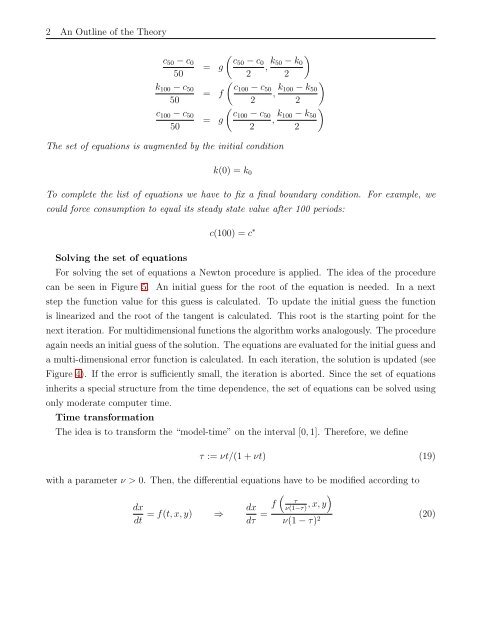
c50 − c0<br />
50<br />
k100 − c50<br />
50<br />
c100 − c50<br />
50<br />
<br />
c50 − c0<br />
= g ,<br />
2<br />
k50<br />
<br />
− k0<br />
2<br />
<br />
c100 − c50<br />
= f ,<br />
2<br />
k100<br />
<br />
− k50<br />
2<br />
<br />
c100 − c50<br />
= g ,<br />
2<br />
k100<br />
<br />
− k50<br />
2<br />
The set of equations is augmented by the initial condition<br />
k(0) = k0<br />
To complete the list of equations we have to fix a final boundary condition. For example, we<br />
could force consumption to equal its steady state value after 100 periods:<br />
Solving the set of equations<br />
c(100) = c ∗<br />
For solving the set of equations a Newton procedure is applied. The idea of the procedure<br />
can be seen in Figure 5. An initial guess for the root of the equation is needed. In a next<br />
step the function value for this guess is calculated. To update the initial guess the function<br />
is linearized and the root of the tangent is calculated. This root is the starting point for the<br />
next iteration. For multidimensional functions the algorithm works analogously. The procedure<br />
again needs an initial guess of the solution. The equations are evaluated for the initial guess and<br />
a multi-dimensional error function is calculated. In each iteration, the solution is updated (see<br />
Figure 4). If the error is sufficiently small, the iteration is aborted. Since the set of equations<br />
inherits a special structure from the time dependence, the set of equations can be solved using<br />
only moderate computer time.<br />
Time transformation<br />
The idea is to transform the “model-time” on the interval [0, 1]. Therefore, we define<br />
τ := νt/(1 + νt) (19)<br />
<strong>with</strong> a parameter ν > 0. Then, the differential equations have to be modified according to<br />
dx<br />
dx<br />
= f(t,x,y) ⇒<br />
dt dτ =<br />
<br />
τ f ν(1−τ) ,x,y<br />
<br />
ν(1 − τ) 2<br />
(20)


