Dynamic Macroeconomic Modeling with Matlab

More documents

Recommendations

Info

2 An Outline of the Theory 2 An Outline of the Theory 2.1 Numerical solution of initial value problems Consider a linear differential equation ˙x(t) = −αx, x(0) = x0, α > 0 (1) A numerical solution of the differential equation is a time vector T = t0,t1,...,tM and a corresponding vector x = x0,x1,...,xM such that x(ti) ≈ xi. A simple numerical method to compute the solution on the interval [0, 10] can be constructed by discretisation. Consider a mesh of time, e.g. T = 0, 0.1, 0.2,...,10. We discretize the differential equation on this mesh according to ⇒ ∆x = −αx (2) ∆t xi − xi−1 ti − ti−1 = −αxi−1 i = 0.1, 0.2,...,10 (3) Then, the numerical solution (or an approximation) can be obtained iteratively by starting at the second mesh point and applying the difference equation from point to point according to xi = xi−1 − (ti − ti−1)αxi−1 i = 0.1, 0.2,...,10 (4) The comparison between numerical and analytical solution can be seen in Figure 1. Note that the numerical solution deviates from the true solution due to linearization. This algorithm is named Explicit Euler method and can easily be generalized to any non- linear differential equation: with g being sufficiently smooth. Then, the algorithm reads ˙x(t) = g(x), x(0) = x0, (5) xi = xi−1 − (ti − ti−1)g(xi−1) i = 0.1, 0.2,...,10 (6) Example 1 (Solow model) The dynamics of the Solow growth model can be summarized by the Fundamental Equation (see Barro and Sala-i-Martin, 2004, p. 30) ˙k = sf(k) − (n + δ)k. (7) Since capital k is the only variable and capital is a state variable, for which the initial value k(0) is given, we could compute transitional dynamics with the explicit Euler method.
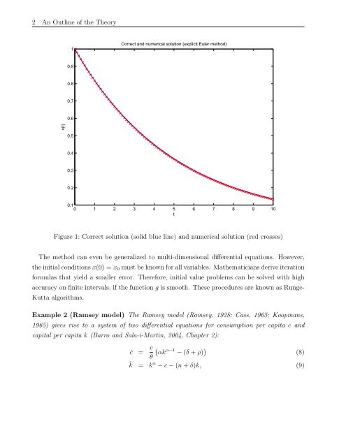
2 An Outline of the Theory x(t) 1 0.9 0.8 0.7 0.6 0.5 0.4 0.3 0.2 Correct and numerical solution (explicit Euler method) 0.1 0 1 2 3 4 5 t 6 7 8 9 10 Figure 1: Correct solution (solid blue line) and numerical solution (red crosses) The method can even be generalized to multi-dimensional differential equations. However, the initial conditions x(0) = x0 must be known for all variables. Mathematicians derive iteration formulas that yield a smaller error. Therefore, initial value problems can be solved with high accuracy on finite intervals, if the function g is smooth. These procedures are known as Runge- Kutta algorithms. Example 2 (Ramsey model) The Ramsey model (Ramsey, 1928; Cass, 1965; Koopmans, 1965) gives rise to a system of two differential equations for consumption per capita c and capital per capita k (Barro and Sala-i-Martin, 2004, Chapter 2): ˙c = c α−1 αk − (δ + ρ) (8) θ ˙k = k α − c − (n + δ)k, (9)
Page 1 and 2: Dynamic Macroeconomic Modeling with
Page 3: 1 Introduction 1 Introduction The a
Page 7 and 8: 2 An Outline of the Theory South-Ea
Page 9 and 10: 2 An Outline of the Theory whereby
Page 11 and 12: 2 An Outline of the Theory c 0.68 0
Page 13 and 14: 2 An Outline of the Theory Figure 5
Page 15 and 16: 3 A Short Introduction to Matlab 3
Page 17 and 18: 3 A Short Introduction to Matlab 4.
Page 19 and 20: 4 Numerical Simulation of Macroecon
Page 37 and 38: References References Ascher, U. M.
Page 39: References Solow, R. M. (1956): “

Dynamic Macroeconomic Modeling with Matlab

You also want an ePaper? Increase the reach of your titles

Delete template?

Save as template?