Dynamic Macroeconomic Modeling with Matlab

More documents

Recommendations

Info

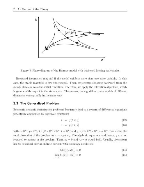
2 An Outline of the Theory Figure 3: Phase diagram of the Ramsey model with backward looking trajectories Backward integration may fail if the model exhibits more than one state variable. In this case, the stable manifold is two-dimensional. Then, trajectories shooting backward from the steady state can miss the initial condition. Therefore, we apply the relaxation algorithm, which is generic with respect to the state space. This means, the algorithm treats models of different dimension conceptually in the same way. 2.3 The Generalized Problem Economic dynamic optimization problems frequently lead to a system of differential equations potentially augmented by algebraic equations: ˙x = f(t,x,y) (12) 0 = g(t,x,y) (13) with xǫR nd, y ǫ R na , f : (R × R nd × R na ) → R nd and g : (R × R nd × R na ) → R na . We define the total dimension of the problem as n := nd + na. The algebraic equations and, hence, y are not required to appear in the problem. Then, na = 0 and nd = n would hold. Usually, the system has to be solved over an infinite horizon with boundary conditions hi(x(0),y(0)) = 0 (14) lim t→∞ hf(x(t),y(t)) = 0 (15)
2 An Outline of the Theory whereby hi : R n → R ni defines ni initial boundary conditions and hf : R n → R nf defines nf final boundary conditions such that ni + nf = nd. The system (12) and (13) taken together with (14) and (15) is labeled two-point boundary value problem, since a system of differential equations has to be solved subject to boundary conditions at the beginning and the end of the time horizon. The specific characteristics of the problem at hand are that equation (12) has to be solved for an infinite time horizon and that the solution is bound to an equation defined by (13). Often, the algebraic equations are differentiated with respect to time such that the resulting system of differential equations is square. However, we do not require this. Example 3 (Ramsey model) The Ramsey model comprise two differential equations: ˙c = c α−1 αk − (δ + ρ) (16) θ ˙k = k α − c − (n + δ)k, (17) one state variable (k) and one control variable (c). Hence, we have n = nd = 2, ni = 1, nf = 1, and na = 0. In case of an infinite time horizon, we require the final boundary conditions to enforce con- vergence towards a curve of dimension nf or less. For many economic applications the desired solution is known to converge towards a single (saddle) point. We include this case in (15). To understand the dynamics around an isolated fixed point, we have to consider the Hartman Grobman theorem Theorem 4 (Linearization Theorem of Hartman and Grobman, Tu (1994)) Let the nonlinear dynamic system ˙x = f(x) have a simple hyperbolic fixed point x ∗ . Let the Jacobian matrix Dxf evaluated at x ∗ have nu eigenvalues with positive real part and ns eigenvalues with negative real part with the corre- sponding eigenspaces N u and N s , respectively (N u ⊕ N s = R n ). Then the following claims hold 1. In the neighborhood U of x ∗ ǫ R n of this equilibrium, the phase portraits of the original system and its linearization ˙x = Dxf|x ∗ · x
Page 1 and 2: Dynamic Macroeconomic Modeling with
Page 3 and 4: 1 Introduction 1 Introduction The a
Page 5 and 6: 2 An Outline of the Theory x(t) 1 0
Page 7: 2 An Outline of the Theory South-Ea
Page 11 and 12: 2 An Outline of the Theory c 0.68 0
Page 13 and 14: 2 An Outline of the Theory Figure 5
Page 15 and 16: 3 A Short Introduction to Matlab 3
Page 17 and 18: 3 A Short Introduction to Matlab 4.
Page 19 and 20: 4 Numerical Simulation of Macroecon
Page 37 and 38: References References Ascher, U. M.
Page 39: References Solow, R. M. (1956): “

Dynamic Macroeconomic Modeling with Matlab

Create successful ePaper yourself

Delete template?

Save as template?