Dynamic Macroeconomic Modeling with Matlab

More documents

Recommendations

Info

2 An Outline of the Theory where α denotes the elasticity of capital in production, n the population growth rate, δ the depreciation rate, ρ the parameter for time preference and θ the inverse of the intertemporal elasticity of substitution, respectively. The interior steady state k ∗ = 1 α 1−α δ+ρ and c ∗ = (k ∗ ) α − (n + δ)k ∗ is saddle point stable. 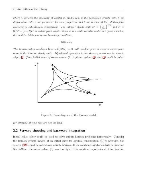Since k is a state variable and c is a jump variable, the model exhibits one initial boundary condition: k(0) = k0 The transversality condition limt→∞ k(t)λ(t) = 0 <strong>with</strong> shadow price λ ensures convergence towards the interior steady state. Adjustment dynamics in the Ramsey model can be seen in Figure 2. If the initial value of consumption c(0) is given, system (8) and (9) could be solved for intervals of time that are not too long. Figure 2: Phase diagram of the Ramsey model 2.2 Forward shooting and backward integration Initial value solver could be used to solve infinite-horizon problems numerically. Consider the Ramsey growth model. If an initial guess for optimal consumption c(0) is provided, the system (8-9) could be solved over a finite horizon. If the solution trajectories drift in direction North-West, the initial value c(0) was too high, if the solution trajectories drift in direction
2 An Outline of the Theory South-East, the initial guess was too low. In an iteration process, the correct value of c(0) could be approximated. This procedure is called “shooting”, since trajectories “shoot” in direction of the steady state until they pass sufficiently close. The problem is that trajectories diverge from the stable manifold (see the graphical illustration of the phase space in Figure 2). Therefore, small changes in the initial value c(0) cause huge deviations from the stable manifold and, hence, the true solution. Even if one would start at the correct initial value, the solution trajectory would diverge from the stable manifold due to small numerical errors. Mathematicians say that the problem is ill conditioned. Brunner and Strulik (2002) suggested to turn the ill conditioned problem into a well conditioned problem by inverting time. This procedure is called backward integration. Consider a system of differential equations <strong>with</strong> xǫR n , g : R n → R n . If we introduce τ := −t, we can write dx dτ ˙x = g(x) (10) dx dt = = −g(x) (11) dt dτ Every vector of the vector field exactly changes its direction. E.g., for the Ramsey model Figure 2 turns into Figure 3. Hence, a stable manifold turns into an unstable manifold and vice versa. The stable solution manifold turns into an unstable manifold. The idea of backward integration is to exploit the information that the economy converges towards a (unique) steady state. Therefore, the solution is traced back from a value close to the steady state to the initial condition. Looking forward, the solution converges to values in the neighborhood of the steady state in finite time. One of these values is chosen as initial value for backward integration. While the initial value c(0) for the original problem can be any value, the initial value for backward integration can be found in a neighborhood of the well-known steady state. In addition, during integration the backward looking trajectories converge towards the solution manifold, instead of divergence of the forward looking trajectories. By reversing the time and thus the flow of the system, a standard forward integration procedure can be used to trace the solution trajectory back to the initial value k(0). It turns out that because of the time reversal the problem is numerically stable. Finally, the trajectory is transformed back into forward looking time by a second time reversal.
Page 1 and 2: Dynamic Macroeconomic Modeling with
Page 3 and 4: 1 Introduction 1 Introduction The a
Page 5: 2 An Outline of the Theory x(t) 1 0
Page 9 and 10: 2 An Outline of the Theory whereby
Page 11 and 12: 2 An Outline of the Theory c 0.68 0
Page 13 and 14: 2 An Outline of the Theory Figure 5
Page 15 and 16: 3 A Short Introduction to Matlab 3
Page 17 and 18: 3 A Short Introduction to Matlab 4.
Page 19 and 20: 4 Numerical Simulation of Macroecon
Page 37 and 38: References References Ascher, U. M.
Page 39: References Solow, R. M. (1956): “

Dynamic Macroeconomic Modeling with Matlab

You also want an ePaper? Increase the reach of your titles

Delete template?

Save as template?