Dynamic Macroeconomic Modeling with Matlab
Dynamic Macroeconomic Modeling with Matlab
Dynamic Macroeconomic Modeling with Matlab
Create successful ePaper yourself
Turn your PDF publications into a flip-book with our unique Google optimized e-Paper software.
4 Numerical Simulation of <strong>Macroeconomic</strong> Models<br />
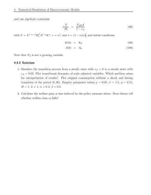
and one algebraic constraint<br />
β Y<br />
HY<br />
= PAηA<br />
1 − sA<br />
<strong>with</strong> Y = L 1−α−β H β<br />
Y A1−α K α , r = α 2 , and π = (1 − α)α Y<br />
A<br />
Note that PA is not a growing variable.<br />
4.4.2 Exercises<br />
K(0) = K0<br />
A(0) = A0<br />
and initial conditions<br />
(98)<br />
(99)<br />
(100)<br />
1. Simulate the transition process from a steady state <strong>with</strong> sA = 0 to a steady state <strong>with</strong><br />
sA = 0.02. Plot transitional dynamics of scale adjusted variables. Which problem arises<br />
for interpretation of results? Plot original consumption <strong>with</strong>out a shock and during<br />
transition of the period [0, 30]. Employ parameter values ρ = 0.05, σ = 1.5, η = 0.15,<br />
H = 1, L = 1, α = 0.4, β = 0.3.<br />
2. Calculate the welfare gain or loss induced by the policy measure above. Does theory tell<br />
whether welfare rises or falls?


