Dynamic Macroeconomic Modeling with Matlab
Dynamic Macroeconomic Modeling with Matlab
Dynamic Macroeconomic Modeling with Matlab
You also want an ePaper? Increase the reach of your titles
YUMPU automatically turns print PDFs into web optimized ePapers that Google loves.
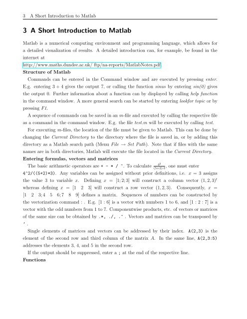
3 A Short Introduction to <strong>Matlab</strong><br />
3 A Short Introduction to <strong>Matlab</strong><br />
<strong>Matlab</strong> is a numerical computing environment and programming language, which allows for<br />
a detailed visualization of results. A detailed introduction can, for example, be found in the<br />
internet at<br />
http://www.maths.dundee.ac.uk/ ftp/na-reports/<strong>Matlab</strong>Notes.pdf.<br />
Structure of <strong>Matlab</strong><br />
Commands can be entered in the Command window and are executed by pressing enter.<br />
E.g. entering 3 + 4 gives the output 7, or calling the function sinus by entering sin(0) gives<br />
the output 0. Further information about a function can by displayed by calling help function<br />
in the command window. A more general search can be started by entering lookfor topic or by<br />
pressing F1.<br />
A sequence of commands can be saved in an m-file and executed by calling the respective file<br />
as a command in the command window. E.g. the file test.m will be executed by calling test.<br />
For executing m-files, the location of the file must be given to <strong>Matlab</strong>. This can be done by<br />
changing the Current Directory to the directory where the file is saved in, or by adding this<br />
directory as a <strong>Matlab</strong> search path (Menu File → Set Path). Note that if files <strong>with</strong> the same<br />
names are in both directories, <strong>Matlab</strong> will execute the file located in the Current Directory.<br />
Entering formulas, vectors and matrices<br />
4 The basic arithmetic operators are + - * / ^. To calculate 2<br />
, one must enter<br />
(5+2)·3<br />
4^2/((5+2)*3). Any variables can be assigned <strong>with</strong>out prior definitions, i.e. x = 3 assigns<br />
the value 3 to variable x. Defining x = [1; 2; 3] will construct a column vector (1, 2, 3) t<br />
whereas defining x = [1 2 3] will construct a row vector (1, 2, 3). Consequently, x =<br />
[1 2 3; 4 5 6; 7 8 9] defines a matrix. Sequences of numbers can be constructed by<br />
the vectorization command : . E.g. [1 : 6] is a vector <strong>with</strong> numbers 1 to 6, and [1 : 2 : 7] is a<br />
vector <strong>with</strong> the odd numbers from 1 to 7. Componentwise products, etc. of vectors or matrices<br />
of the same size can be obtained by .*, ./, .^ . Vectors and matrices can be transposed by<br />
’ .<br />
Single elements of matrices and vectors can be addressed by their index. A(2,3) is the<br />
element of the second row and third column of the matrix A. In the same line, A(2,3:5)<br />
addresses the elements 3, 4, and 5 in the second row.<br />
If the output should be suppressed, enter a ; at the end of the respective line.<br />
Functions


