The UMIST-N Near-Wall Treatment Applied to Periodic Channel Flow

CHAPTER 5. RESULTS 72
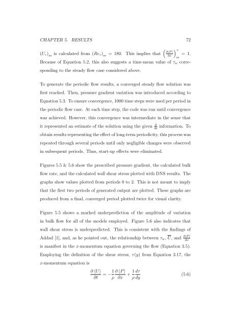
(Uτ) ss is calculated from (Reτ) ss = 180. This implies that
+
∂〈P 〉
∂x
ss
= 1.
Because of Equation 5.2, this also suggests a time-mean value of τw corre-
sponding to the steady flow case considered above.
To generate the periodic flow results, a converged steady flow solution was
first reached. Then, pressure gradient variation was introduced according to
Equation 5.3. To ensure convergence, 1000 time steps were used per period in
the periodic flow case. At each time step, the code was run until convergence
was achieved. However, this convergence was intermediate in the sense that
it represented an estimate of the solution using the given ∂
∂t
information. To
obtain results representing the effect of long-term periodicity, this process was
repeated through several periods until only negligible changes were observed
in subsequent periods. Thus, start-up effects were eliminated.
Figures 5.5 & 5.6 show the prescribed pressure gradient, the calculated bulk
flow rate, and the calculated wall shear stress plotted with DNS results. The
graphs show values plotted from periods 0 to 2. This is not meant to imply
that the first two periods of generated output are plotted. These graphs are
produced from a final, converged period plotted twice for visual clarity.
Figure 5.5 shows a marked underprediction of the amplitude of variation
in bulk flow for all of the models employed. Figure 5.6 also indicates that
wall shear stress is underpredicted. This is consistent with the findings of
Addad [1], and, as he pointed out, the relationship between τw, U, and
is manifest in the x-momentum equation governing the flow (Equation 3.5).
Employing the definition of the shear stress, τ(y) from Equation 3.17, the
x-momentum equation is
∂ 〈U〉
∂t
∂ 〈P 〉
= −1
ρ ∂x
1 dτ
+
ρ dy
∂〈P 〉
∂x
(5.6)