Modeling and Optimization of the Vortex Tube with ... - TU Berlin
Modeling and Optimization of the Vortex Tube with ... - TU Berlin
Modeling and Optimization of the Vortex Tube with ... - TU Berlin

You also want an ePaper? Increase the reach of your titles
YUMPU automatically turns print PDFs into web optimized ePapers that Google loves.
Energy Research Journal 1 (2): 193-196, 2010<br />
ISSN 1949-0151<br />
© 2010 Science Publications<br />
<strong>Modeling</strong> <strong>and</strong> <strong>Optimization</strong> <strong>of</strong> <strong>the</strong> <strong>Vortex</strong> <strong>Tube</strong> <strong>with</strong><br />
Computational Fluid Dynamic Analysis<br />
K.K. Zin, A. Hansske <strong>and</strong> F. Ziegler<br />
Department <strong>of</strong> Energy Conversion Engineering,<br />
Technical University <strong>of</strong> <strong>Berlin</strong>, Sekr. KT 2,<br />
Marchstraße 18, 10587 <strong>Berlin</strong>, Germany<br />
Abstract: Problem statement: This study illustrated <strong>the</strong> influence <strong>of</strong> <strong>the</strong> Length to Diameter (L/D)<br />
on <strong>the</strong> fluid flow characteristics inside <strong>the</strong> counter-flow Ranque-Hilsch vortex tube predicted by<br />
Computational Fluid Dynamic (CFD) <strong>and</strong> validated through experiment. Approach: The swirl<br />
velocity, axial velocity, radial velocity component <strong>and</strong> also secondary circulation flow (back-flow)<br />
along <strong>with</strong> <strong>the</strong> pressure <strong>with</strong>in <strong>the</strong> vortex tube were simulated <strong>and</strong> proved. Results: The st<strong>and</strong>ard kepsilon<br />
turbulence model which is one <strong>of</strong> <strong>the</strong> st<strong>and</strong>ard turbulence models <strong>of</strong> FLUENT TM was being<br />
used. As a first step, results <strong>of</strong> simulation will be presented also <strong>with</strong> varying amounts <strong>of</strong> cold faction.<br />
Conclusion/Recommendations: In <strong>the</strong> present study, <strong>the</strong> velocity <strong>and</strong> <strong>the</strong> pressure were investigated<br />
along <strong>the</strong> axial <strong>and</strong> radial directions to underst<strong>and</strong> <strong>the</strong> flow behavior inside <strong>the</strong> tube.<br />
Key words: Ranque-Hilsch vortex tube, CFD simulation, design parameters, k-epsilon model<br />
INTRODUCTION<br />
The Ranque-Hilsch vortex tube having, relatively<br />
simple geometry, no moving mechanical parts, was<br />
invented by Ranque (Hansske et al., 2007) (Fig. 1).<br />
Many investigators have suggested various <strong>the</strong>ories to<br />
explain <strong>the</strong> Ranque effect. Most important seems to be a<br />
study by Ahlborn et al. (1998) in which a <strong>the</strong>ory <strong>of</strong><br />
temperature separation based on a heat pump mechanism<br />
which is enabled by a secondary circulation flow is<br />
proposed. However, till today no exact description has<br />
emerged to explain <strong>the</strong> phenomenon satisfactorily. Thus<br />
much <strong>of</strong> <strong>the</strong> design <strong>and</strong> development <strong>of</strong> vortex tubes has<br />
been based on empirical correlations only leaving much<br />
room for optimization <strong>of</strong> critical parameters. <strong>Vortex</strong><br />
flows or swirl flows have been <strong>of</strong> considerable interest<br />
over <strong>the</strong> past decades because <strong>of</strong> <strong>the</strong>ir occurrence in<br />
industrial applications, such as furnaces, gas-turbine<br />
combustors <strong>and</strong> dust collectors (Fig. 2). The vortex tube<br />
has been used in industrial applications <strong>of</strong> cooling <strong>and</strong><br />
heating processes because <strong>of</strong> being a simple, compact,<br />
light <strong>and</strong> quiet (in operation) device (Bruno, 1992).<br />
MATERIALS AND METHODS<br />
Numerical modeling: A numerical model <strong>of</strong> <strong>the</strong><br />
Ranque-Hilsch vortex tube has been created by using <strong>the</strong><br />
FLUENT TM s<strong>of</strong>tware package. The model is threedimensional,<br />
steady state, source-free <strong>and</strong> employs <strong>the</strong><br />
st<strong>and</strong>ard k-epsilon turbulence model. The RNG k-epsilon<br />
turbulence model <strong>and</strong> more advanced turbulence models<br />
such as <strong>the</strong> Reynolds stress equations were also<br />
investigated, but <strong>the</strong>se models could not be made to<br />
converge for this simulation yet.<br />
The equation for conservation <strong>of</strong> mass <strong>and</strong><br />
momentum are as follow:<br />
∂ P r<br />
+ ∇. ( ρυ ) = 0<br />
∂t<br />
Corresponding Author: K.K. Zin, Department <strong>of</strong> Energy Conversion Engineering, Technical University <strong>of</strong> <strong>Berlin</strong>, Sekr. KT 2,<br />
Marchstraße 18, 10587 <strong>Berlin</strong>, Germany Tel: ++49 (0) 30/314 24614 Fax: ++49 (0) 30/314 22253<br />
193<br />
(1)<br />
∂p<br />
r r r r r<br />
( ρυ ) + ∇. ( ρυυ ) = −∇ p + ∇ . (t) + ρ g + F<br />
(2)<br />
∂t<br />
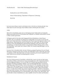
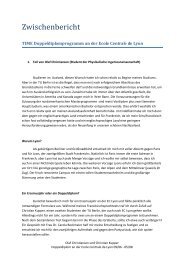
Fig. 1: Schematic flow pattern <strong>of</strong> Ranque-Hilsch tube
Fig. 2: Schematic velocity distribution <strong>of</strong> Ranque-<br />
Hilsch tube (Behera et al., 2005)<br />
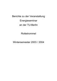
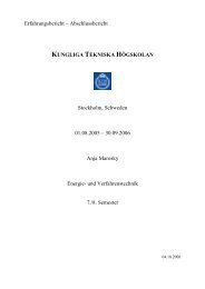
Fig. 3: CFD mesh grid showing <strong>of</strong> <strong>the</strong> Ranque-Hilsch<br />
tube <strong>with</strong> L/D ratio is 5<br />
The turbulence kinetic energy, k <strong>and</strong> its rate <strong>of</strong><br />
dissipation, ε, are obtained from <strong>the</strong> following transport<br />
equations:<br />
∂ ∂ ∂ ⎡⎛ μ ⎞ t ∂k<br />
⎤<br />
( ρ k) + ( ρ ku i ) = ⎢⎜ μ + ⎟ ⎥ + G k +<br />
∂t ∂x i ∂x j ⎢⎣ ⎝ σ k ⎠ ∂x<br />
j ⎥⎦<br />
G − ρ ∈ − Y + S<br />
b M k<br />
∂ ∂ ∂ ⎡⎛ μ ⎞ ∂ ∈ ⎤<br />
( ) ( u )<br />
∂t ∂x ∂x ⎢⎣ ⎝ σ ⎠ ∂x<br />
⎥⎦<br />
ρ ∈ + ρ ∈ i = ⎢⎜ μ + t<br />
⎟ ⎥ +<br />
i j ∈ j<br />
2<br />
∈ ∈<br />
C (G + C G ) − C ρ + S<br />
k k<br />
1ε k 3∈ b 2∈<br />
∈<br />
Energy Rec. J. 1 (2): 193-196, 2010<br />
(3)<br />
(4)<br />
The turbulent (or eddy) viscosity, µt, is computed<br />
by combining k <strong>and</strong> ε as follows:<br />
2<br />
k<br />
μ t = ρCμ<br />
∈<br />
(5)<br />
The model constants C1ε, C2ε, Cµ, σk <strong>and</strong> σε have<br />
<strong>the</strong> following default values (FLUENT TM user guide):<br />
C1ε = 1.44, C2ε = 1.92, Cµ = 0.09, σk = 1.0, σε = 1.3<br />
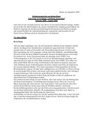
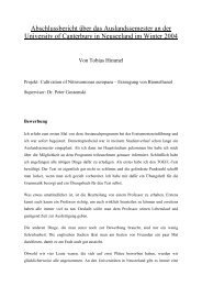
(a)<br />
(b)<br />
Fig. 4: Axial <strong>and</strong> radial velocity components <strong>with</strong><br />
radial distance (where Z is <strong>the</strong> axial distance<br />
along <strong>the</strong> vortex tube)<br />
The working fluid (ideal gas) is <strong>the</strong> working fluid.<br />
Physical modeling <strong>of</strong> vortex tube: The geometric<br />
model has been carried out <strong>with</strong> <strong>the</strong> GAMBIT<br />
194<br />
TM mesh<br />
generation code. A mesh consisting <strong>of</strong> 170022 grid nodes<br />
is shown in Fig. 3. The inlet <strong>of</strong> 3×10 mm <strong>and</strong> <strong>the</strong><br />
diameter <strong>of</strong> vortex tube, D = 32 mm are kept constant in<br />
<strong>the</strong> analysis. The L/D ratio assumed for <strong>the</strong> studies<br />
ranged from 5-20.<br />
Variations <strong>of</strong> <strong>the</strong> velocity components along axial<br />
<strong>and</strong> radial direction are shown in Fig. 4a <strong>and</strong> b. The<br />
velocity along <strong>the</strong> axial direction show <strong>the</strong> evidence <strong>of</strong><br />
<strong>the</strong> forced <strong>and</strong> free vortex zone inside <strong>the</strong> tube <strong>and</strong> <strong>the</strong><br />
existence <strong>of</strong> secondary flow from <strong>the</strong> inlet to <strong>the</strong> cold end<br />
<strong>and</strong> till to <strong>the</strong> stagnation point.
Energy Rec. J. 1 (2): 193-196, 2010<br />
Table 1: Fixed <strong>and</strong> variable parameters for <strong>the</strong> simulation<br />
Inlet mass flow Inlet pressure Pin Inlet temperature Cold exit pressure Cold mass fraction Length <strong>and</strong><br />
(kg sec −1 ) (kPa) (absolute) Tin (K) (total) Pc (kPa) (absolute) Yc diameter ratio<br />
-----------------------------------------------------------------------------------------------------------------------------------------------------------------------<br />
0.015 280.000 294 101.325 0.1, 0.2, 0.35, 0.5, 0.7 5, 10, 15, 20<br />
Boundary condition: Boundary conditions for <strong>the</strong><br />
model were defined based on <strong>the</strong> experimental<br />
measurements. The inlet is modeled as a mass flow inlet;<br />
<strong>the</strong> mass flow rate, total temperature, direction vector<br />
<strong>and</strong> turbulence parameters were specified. The cold <strong>and</strong><br />
hot outlets are determined as pressure outlets using<br />
measured values <strong>of</strong> <strong>the</strong> static pressure (Skye et al.,<br />
2006).<br />
Study <strong>of</strong> grid dependence: The fixed <strong>and</strong> variable<br />
parameters for <strong>the</strong> numerical analysis are listed in Table 1.<br />
To eliminate <strong>the</strong> errors due to coarseness <strong>of</strong> grid,<br />
analysis has been carried out for different average unit<br />
cell volumes in a vortex tube <strong>of</strong> L/D = 5. For a smaller<br />
mesh size <strong>the</strong>n reported about <strong>the</strong> solution is<br />
independence from <strong>the</strong> grid size.<br />
RESULTS<br />
CFD analyses were carried out for a 32 mm<br />
diameter vortex tube <strong>with</strong> L/D <strong>of</strong> 5, 10, 15 <strong>and</strong> 20<br />
verify <strong>the</strong> existence <strong>of</strong> a secondary circulation flow, a<br />
stagnation point. And also <strong>with</strong> <strong>the</strong> varying amount <strong>of</strong><br />
cold fraction (i.e., mass flow <strong>of</strong> cold outlet in relation<br />
to <strong>the</strong> inlet) 0.1, 0.2, 0.35, 0.5, 0.7 has been varied to<br />
investigate <strong>the</strong> variation <strong>of</strong> static <strong>and</strong> total pressure as<br />
well as <strong>the</strong> velocity components <strong>of</strong> <strong>the</strong> particle as it<br />
progresses in <strong>the</strong> tube, starting from <strong>the</strong> entry through<br />
to <strong>the</strong> cold <strong>and</strong> hot exit by tracking <strong>the</strong> particles to<br />
underst<strong>and</strong> <strong>the</strong> flow phenomenon inside <strong>the</strong> vortex<br />
tube.<br />
The improvement <strong>of</strong> <strong>the</strong> CFD result will be<br />
achieved by improving <strong>the</strong> calculation <strong>of</strong> <strong>the</strong> pressure<br />
loss along <strong>the</strong> tube.<br />
DISCUSSION<br />
Velocity components <strong>and</strong> secondary circulation<br />
flow: The velocity magnitude along <strong>the</strong> center line <strong>of</strong><br />
<strong>the</strong> vortex tube <strong>with</strong> corresponding L/D ratio is shown<br />
in Fig. 5. The velocity magnitude comes to zero at an<br />
axial distance between 100 <strong>and</strong> 200 mm from <strong>the</strong> cold<br />
exit. The stagnation point is almost independent from<br />
<strong>the</strong> tube length which are after <strong>the</strong> stagnation points<br />
<strong>the</strong>re is a vortex <strong>the</strong> structure is similar to Görtler<br />
vortice because <strong>of</strong> <strong>the</strong> velocity distribution <strong>of</strong> <strong>the</strong><br />
turbulent swirl flow <strong>with</strong> secondary circulation.<br />
195<br />
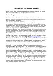
Fig. 5: Velocity magnitude along <strong>the</strong> center line <strong>of</strong> <strong>the</strong><br />
vortex <strong>with</strong> different L/D ratio<br />
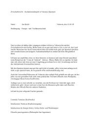
(a)<br />
(b)<br />
Fig. 6: Axial absolute pressure gradient along <strong>the</strong> length<br />
<strong>of</strong> <strong>the</strong> tube
Pressure components <strong>and</strong> experimental<br />
verification: A parametric study was carried out to<br />
investigate <strong>the</strong> effect <strong>of</strong> varying <strong>the</strong> mass flow rate at<br />
<strong>the</strong> cold <strong>and</strong> hot exits on <strong>the</strong> pressure <strong>and</strong> flow<br />
separation. For a simulated <strong>and</strong> measured L/D ratio <strong>of</strong><br />
20 <strong>and</strong> <strong>the</strong> cold mass fraction 0.1, 0.2. 0.35, 0.5 <strong>and</strong><br />
0.7, <strong>the</strong> results are shown in Fig. 6a <strong>and</strong> b. There is<br />
only fair agreement in <strong>the</strong> total pressures obtained<br />
through experiment <strong>and</strong> by CFD simulation.<br />
CONCLUSION<br />
A three-dimensional numerical model <strong>of</strong> <strong>the</strong><br />
Ranque-Hilsch vortex has been established to analyze<br />
<strong>the</strong> flow inside <strong>the</strong> tube. The studies have confirmed <strong>the</strong><br />
presence <strong>of</strong> a secondary flow. The stagnation point<br />
inside <strong>the</strong> tube is almost independent <strong>of</strong> <strong>the</strong> tube length.<br />
The velocity pr<strong>of</strong>iles in <strong>the</strong> radial direction at different<br />
axial position show that <strong>the</strong> flow in <strong>the</strong> vortex tube is<br />
largely affected by <strong>the</strong> forced vortex. However, <strong>the</strong><br />
disagreement <strong>of</strong> measured <strong>and</strong> simulated pressure along<br />
<strong>the</strong> tube length shows that <strong>the</strong> model still have to be<br />
improve.<br />
REFERENCES<br />
Ahlborn, B.K., J.U. Keller <strong>and</strong> E. Rebhan, 1998. The<br />
heat pump in a vortex tube. J. Non-equilib.<br />
Thermodyn., 23: 159-165.<br />
http://cat.inist.fr/?aModele=afficheN&cpsidt=1053<br />
7580<br />
Bruno, T.J., 1992. Applications <strong>of</strong> <strong>the</strong> vortex tube in<br />
chemical analysis. Process Control Qual., 3: 195-207.<br />
Energy Rec. J. 1 (2): 193-196, 2010<br />
196<br />
Behera, U., P.J. Paul, S. Kasthurirengan, R. Karunanithi<br />
<strong>and</strong> S.N. Ram et al., 2005. CFD analysis <strong>and</strong><br />
experimental investigations towards optimizing <strong>the</strong><br />
parameters <strong>of</strong> Ranque-Hilsch vortex tube. Int. J.<br />
Heat Mass Transfer, 48: 1961-1973. DOI:<br />
10.1016/j.ijheatmasstransfer.2004.12.046<br />
Hansske, A., D. Müller, R. Streblow <strong>and</strong> F. Ziegler,<br />
2007. Experiments <strong>and</strong> simulation <strong>of</strong> a vortex<br />
tube. ETA. http://www.eta.tuberlin.de/fileadmin/a33371300/Redakteurbereich/<br />
Forschung/Abstracts/Experiments_<strong>and</strong>_Simulatio<br />
n_<strong>of</strong>_a_<strong>Vortex</strong>_<strong>Tube</strong>_Abstract.pdf<br />
Skye, H.M., G.F. Nellis <strong>and</strong> S.A. Klein, 2006.<br />
Comparison <strong>of</strong> CFD analysis to empirical data in a<br />
commercial vortex tube. Int. J. Refrig., 29: 71-80.<br />
DOI: 10.1016/j.ijrefrig.2005.05.004