GAMS/PATH User Guide Version 4.3

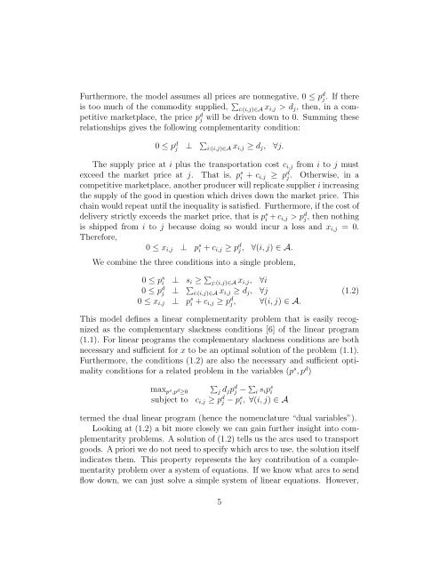
Furthermore, the model assumes all prices are nonnegative, 0 ≤ p d j .Ifthere
is too much of the commodity supplied,
i:(i,j)∈A xi,j >dj, then, in a competitive
marketplace, the price p d j will be driven down to 0. Summing these
relationships gives the following complementarity condition:
0 ≤ p d j
⊥
i:(i,j)∈A xi,j ≥ dj, ∀j.
The supply price at i plus the transportation cost ci,j from i to j must
exceed the market price at j. That is, ps i + ci,j ≥ pd j. Otherwise, in a
competitive marketplace, another producer will replicate supplier i increasing
the supply of the good in question which drives down the market price. This
chain would repeat until the inequality is satisfied. Furthermore, if the cost of
delivery strictly exceeds the market price, that is ps i + ci,j >pd j , then nothing
is shipped from i to j because doing so would incur a loss and xi,j =0.
Therefore,
0 ≤ xi,j ⊥ ps i + ci,j ≥ pd j , ∀(i, j) ∈A.
We combine the three conditions into a single problem,
0 ≤ ps i ⊥ si ≥
0 ≤ p
j:(i,j)∈A xi,j, ∀i
d j ⊥
0 ≤ xi,j ⊥
i:(i,j)∈A xi,j ≥ dj,
p
∀j
s i + ci,j ≥ pd j, ∀(i, j) ∈A.
(1.2)
This model defines a linear complementarity problem that is easily recognized
as the complementary slackness conditions [6] of the linear program
(1.1). For linear programs the complementary slackness conditions are both
necessary and sufficient for x to be an optimal solution of the problem (1.1).
Furthermore, the conditions (1.2) are also the necessary and sufficient optimality
conditions for a related problem in the variables (p s ,p d )
maxps ,pd≥0 subject to ci,j ≥ pd j − psi
j djpd j −
i sips i
, ∀(i, j) ∈A
termed the dual linear program (hence the nomenclature “dual variables”).
Looking at (1.2) a bit more closely we can gain further insight into complementarity
problems. A solution of (1.2) tells us the arcs used to transport
goods. A priori we do not need to specify which arcs to use, the solution itself
indicates them. This property represents the key contribution of a complementarity
problem over a system of equations. If we know what arcs to send
flow down, we can just solve a simple system of linear equations. However,
5