

GAMS/PATH User Guide Version 4.3
GAMS/PATH User Guide Version 4.3
GAMS/PATH User Guide Version 4.3

You also want an ePaper? Increase the reach of your titles
YUMPU automatically turns print PDFs into web optimized ePapers that Google loves.
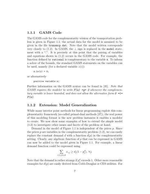
1.1.1 <strong>GAMS</strong> Code<br />
The <strong>GAMS</strong> code for the complementarity version of the transportation problem<br />
is given in Figure 1.1; the actual data for the model is assumed to be<br />
given in the file transmcp.dat. Note that the model written corresponds<br />
very closely to (1.2). In <strong>GAMS</strong>, the ⊥ sign is replaced in the model statement<br />
with a “.”. It is precisely at this point that the pairing of variables<br />
and equations shown in (1.2) occurs in the <strong>GAMS</strong> code. For example, the<br />
function defined by rational is complementary to the variable x. Toinform<br />
a solver of the bounds, the standard <strong>GAMS</strong> statements on the variables can<br />
be used, namely (for a declared variable z(i)):<br />
z.lo(i) = 0;<br />
or alternatively<br />
positive variable z;<br />
Further information on the <strong>GAMS</strong> syntax can be found in [35]. Note that<br />
<strong>GAMS</strong> requires the modeler to write F(z) =g= 0 whenever the complementary<br />
variable is lower bounded, and does not allow the alternative form 0 =l=<br />
F(z).<br />
1.1.2 Extension: Model Generalization<br />
While many interior point methods for linear programming exploit this complementarity<br />
framework (so-called primal-dual methods [37]), the real power<br />
of this modeling format is the new problem instances it enables a modeler<br />
to create. We now show some examples of how to extend the simple model<br />
(1.2) to investigate other issues and facets of the problem at hand.<br />
Demand in the model of Figure 1.1 is independent of the prices p. Since<br />
the prices p are variables in the complementarity problem (1.2), we can easily<br />
replace the constant demand d with a function d(p) in the complementarity<br />
setting. Clearly, any algebraic function of p that can be expressed in <strong>GAMS</strong><br />
can now be added to the model given in Figure 1.1. For example, a linear<br />
demand function could be expressed using<br />
<br />
xi,j ≥ dj(1 − p<br />
i:(i,j)∈A<br />
d j ), ∀j.<br />
Note that the demand is rather strange if p d j exceeds 1. Other more reasonable<br />
examples for d(p) are easily derived from Cobb-Douglas or CES utilities. For<br />
7


