GAMS Tutorial

2
A GAMS Tutorial by Richard E. Rosenthal
2.1 Introduction
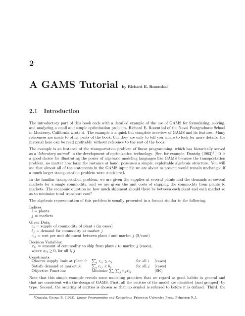
The introductory part of this book ends with a detailed example of the use of GAMS for formulating, solving,
and analyzing a small and simple optimization problem. Richard E. Rosenthal of the Naval Postgraduate School
in Monterey, California wrote it. The example is a quick but complete overview of GAMS and its features. Many
references are made to other parts of the book, but they are only to tell you where to look for more details; the
material here can be read profitably without reference to the rest of the book.
The example is an instance of the transportation problem of linear programming, which has historically served
as a ’laboratory animal’ in the development of optimization technology. [See, for example, Dantzig (1963) 1 .] It is
a good choice for illustrating the power of algebraic modeling languages like GAMS because the transportation
problem, no matter how large the instance at hand, possesses a simple, exploitable algebraic structure. You will
see that almost all of the statements in the GAMS input file we are about to present would remain unchanged if
a much larger transportation problem were considered.
In the familiar transportation problem, we are given the supplies at several plants and the demands at several
markets for a single commodity, and we are given the unit costs of shipping the commodity from plants to
markets. The economic question is: how much shipment should there be between each plant and each market so
as to minimize total transport cost?
The algebraic representation of this problem is usually presented in a format similar to the following.
Indices:
i = plants
j = markets
Given Data:
ai = supply of commodity of plant i (in cases)
bj = demand for commodity at market j
cij = cost per unit shipment between plant i and market j ($/case)
Decision Variables:
xij = amount of commodity to ship from plant i to market j (cases),
where xij ≥ 0, for all i, j
Constraints:
Observe supply limit at plant i:
j xij ≤ aj for all i (cases)
Satisfy demand at market j:
i xij ≥ bj for all j (cases)
Objective Function: Minimize
i j cijxij
($K)
Note that this simple example reveals some modeling practices that we regard as good habits in general and
that are consistent with the design of GAMS. First, all the entities of the model are identified (and grouped) by
type. Second, the ordering of entities is chosen so that no symbol is referred to before it is defined. Third, the
1 Dantzig, George B. (1963). Linear Programming and Extensions, Princeton University Press, Princeton N.J.

6 A GAMS Tutorial by Richard E. Rosenthal
units of all entities are specified, and, fourth, the units are chosen to a scale such that the numerical values to be
encountered by the optimizer have relatively small absolute orders of magnitude. (The symbol $K here means
thousands of dollars.)
The names of the types of entities may differ among modelers. For example, economists use the terms exogenous
variable and endogenous variable for given data and decision variable, respectively. In GAMS, the terminology
adopted is as follows: indices are called sets, given data are called parameters, decision variables are called
variables, and constraints and the objective function are called equations.
The GAMS representation of the transportation problem closely resembles the algebraic representation above.
The most important difference, however, is that the GAMS version can be read and processed by the computer.
Plants Shipping Distances to Markets (1000 miles) Supplies
New York Chicago Topeka
Seattle 2.5 1.7 1.8 350
San Diego 2.5 1.8 1.4 600
Demands 325 300 275
Table 2.1: Data for the transportation problem (adapted from Dantzig, 1963)
As an instance of the transportation problem, suppose there are two canning plants and three markets, with the
data given in table 2.1. Shipping distances are in thousands of miles, and shipping costs are assumed to be $90.00
per case per thousand miles. The GAMS representation of this problem is as follows:
Sets
i canning plants / seattle, san-diego /
j markets / new-york, chicago, topeka / ;
Parameters
a(i) capacity of plant i in cases
/ seattle 350
san-diego 600 /
b(j) demand at market j in cases
/ new-york 325
chicago 300
topeka 275 / ;
Table d(i,j) distance in thousands of miles
new-york chicago topeka
seattle 2.5 1.7 1.8
san-diego 2.5 1.8 1.4 ;
Scalar f freight in dollars per case per thousand miles /90/ ;
Parameter c(i,j) transport cost in thousands of dollars per case ;
c(i,j) = f * d(i,j) / 1000 ;
Variables
x(i,j) shipment quantities in cases
z total transportation costs in thousands of dollars ;
Positive Variable x ;
Equations
cost define objective function
supply(i) observe supply limit at plant i
demand(j) satisfy demand at market j ;
cost .. z =e= sum((i,j), c(i,j)*x(i,j)) ;
supply(i) .. sum(j, x(i,j)) =l= a(i) ;

2.2 Structure of a GAMS Model 7
demand(j) .. sum(i, x(i,j)) =g= b(j) ;
Model transport /all/ ;
Solve transport using lp minimizing z ;
Display x.l, x.m ;
If you submit a file containing the statements above as input to the GAMS program, the transportation model
will be formulated and solved. Details vary on how to invoke GAMS on different of computers, but the simplest
(’no frills’) way to call GAMS is to enter the word GAMS followed by the input file’s name. You will see a number
of terse lines describing the progress GAMS is making, including the name of the file onto which the output is
being written. When GAMS has finished, examine this file, and if all has gone well the optimal shipments will
be displayed at the bottom as follows.
new-york chicago topeka
seattle 50.000 300.000
san-diego 275.000 275.000
You will also receive the marginal costs (simplex multipliers) below.
chicago topeka
seattle 0.036
san-diego 0.009
These results indicate, for example, that it is optimal to send nothing from Seattle to Topeka, but if you insist
on sending one case it will add .036 $K (or $36.00) to the optimal cost. (Can you prove that this figure is correct
from the optimal shipments and the given data?)
2.2 Structure of a GAMS Model
For the remainder of the tutorial, we will discuss the basic components of a GAMS model, with reference to the
example above. The basic components are listed in table 2.2.
There are optional input components, such as edit checks for bad data and requests for customized reports of
results. Other optional advanced features include saving and restoring old models, and creating multiple models
in a single run, but this tutorial will discuss only the basic components.
Before treating the individual components, we give a few general remarks.
1. A GAMS model is a collection of statements in the GAMS Language. The only rule governing the
ordering of statements is that an entity of the model cannot be referenced before it is declared to exist.
2. GAMS statements may be laid out typographically in almost any style that is appealing to the user.
Multiple lines per statement, embedded blank lines, and multiple statements per line are allowed. You
will get a good idea of what is allowed from the examples in this tutorial, but precise rules of the road
are given in the next Chapter.
3. When you are a beginning GAMS user, you should terminate every statement with a semicolon, as in
our examples. The GAMS compiler does not distinguish between upper-and lowercase letters, so you
are free to use either.
4. Documentation is crucial to the usefulness of mathematical models. It is more useful (and most likely
to be accurate) if it is embedded within the model itself rather than written up separately. There are
at least two ways to insert documentation within a GAMS model. First, any line that starts with an
asterisk in column 1 is disregarded as a comment line by the GAMS compiler. Second, perhaps more
important, documentary text can be inserted within specific GAMS statements. All the lowercase
words in the transportation model are examples of the second form of documentation.

8 A GAMS Tutorial by Richard E. Rosenthal
Inputs:
• Sets
Declaration
Assignment of members
• Data (Parameters, Tables, Scalars)
Declaration
Assignment of values
• Variables
Declaration
Assignment of type
• Assignment of bounds and/or initial values (optional)
• Equations
Declaration
Definition
• Model and Solve statements
• Display statement (optional)
Outputs:
• Echo Print
• Reference Maps
• Equation Listings
• Status Reports
• Results
Table 2.2: The basic components of a GAMS model
5. As you can see from the list of input components above, the creation of GAMS entities involves two
steps: a declaration and an assignment or definition. Declaration means declaring the existence of
something and giving it a name. Assignment or definition means giving something a specific value or
form. In the case of equations, you must make the declaration and definition in separate GAMS
statements. For all other GAMS entities, however, you have the option of making declarations and
assignments in the same statement or separately.
6. The names given to the entities of the model must start with a letter and can be followed by up to
thirty more letters or digits.
2.3 Sets
Sets are the basic building blocks of a GAMS model, corresponding exactly to the indices in the algebraic
representations of models. The Transportation example above contains just one Set statement:
Sets
i canning plants / seattle, san-diego /
j markets / new-york, chicago, topeka / ;
The effect of this statement is probably self-evident. We declared two sets and gave them the names i and j. We
also assigned members to the sets as follows:
i = {Seattle, San Diego}
j = {New York, Chicago, Topeka}.
You should note the typographical differences between the GAMS format and the usual mathematical format
for listing the elements of a set. GAMS uses slashes ’/’ rather than curly braces ’{}’ to delineate the set simply

2.4 Data 9
because not all computer keyboards have keys for curly braces. Note also that multiword names like ’New York’
are not allowed, so hyphens are inserted.
The lowercase words in the sets statement above are called text. Text is optional. It is there only for internal
documentation, serving no formal purpose in the model. The GAMS compiler makes no attempt to interpret the
text, but it saves the text and ’parrots’ it back to you at various times for your convenience.
It was not necessary to combine the creation of sets i and j in one statement. We could have put them into
separate statements as follows:
Set i canning plants / seattle, san-diego / ;
Set j markets / new-york, chicago, topeka / ;
The placement of blank spaces and lines (as well as the choice of upper- or lowercase) is up to you. Each GAMS
user tends to develop individual stylistic conventions. (The use of the singular set is also up to you. Using set
in a statement that makes a single declaration and sets in one that makes several is good English, but GAMS
treats the singular and plural synonymously.)
A convenient feature to use when you are assigning members to a set is the asterisk. It applies to cases when the
elements follow a sequence. For example, the following are valid set statements in GAMS.
Set t time periods /1991*2000/;
Set m machines /mach1*mach24/;
Here the effect is to assign
t = {1991,1992,1993, ....., 2000}
m = {mach1, mach2,......, mach24}.
Note that set elements are stored as character strings, so the elements of t are not numbers.
Another convenient feature is the alias statement, which is used to give another name to a previously declared
set. In the following example:
Alias (t,tp);
the name tp is like a t ′ in mathematical notation. It is useful in models that are concerned with the interactions
of elements within the same set.
The sets i, j, t, and m in the statements above are examples of static sets, i.e., they are assigned their members
directly by the user and do not change. GAMS has several capabilities for creating dynamic sets, which acquire
their members through the execution of set-theoretic and logical operations. Dynamic sets are discussed in Chapter
12, page117. Another valuable advanced feature is multidimensional sets, which are discussed in Section 4.5,
page 39.
2.4 Data
The GAMS model of the transportation problem demonstrates all of the three fundamentally different formats
that are allowable for entering data. The three formats are:
• Lists
• Tables
• Direct assignments
The next three sub-sections will discuss each of these formats in turn.

10 A GAMS Tutorial by Richard E. Rosenthal
2.4.1 Data Entry by Lists
The first format is illustrated by the first Parameters statement of the example, which is repeated below.
Parameters
a(i) capacity of plant i in cases
/ seattle 350
san-diego 600 /
b(j) demand at market j in cases
/ new-york 325
chicago 300
topeka 275 / ;
This statement has several effects. Again, they may be self-evident, but it is worthwhile to analyze them in
detail. The statement declares the existence of two parameters, gives them the names a and b, and declares their
domains to be i and j, respectively. (A domain is the set, or tuple of sets, over which a parameter, variable, or
equation is defined.) The statement also gives documentary text for each parameter and assigns values of a(i)
and b(j) for each element of i and j. It is perfectly acceptable to break this one statement into two, if you
prefer, as follows.
Parameters a(i) capacity of plant i in cases
/ seattle 350
san-diego 600 / ;
Parameters b(j) demand at market j in cases
/ new-york 325
chicago 300
topeka 275 / ;
Here are some points to remember when using the list format.
1. The list of domain elements and their respective parameter values can be laid out in almost any way
you like. The only rules are that the entire list must be enclosed in slashes and that the element-value
pairs must be separated by commas or entered on separate lines.
2. There is no semicolon separating the element-value list from the name, domain, and text that precede
it. This is because the same statement is being used for declaration and assignment when you use the
list format. (An element-value list by itself is not interpretable by GAMS and will result in an error
message.)
3. The GAMS compiler has an unusual feature called domain checking, which verifies that each domain
element in the list is in fact a member of the appropriate set. For example, if you were to spell ’Seattle’
correctly in the statement declaring Set i but misspell it as ’Seatle’ in a subsequent element-value list,
the GAMS compiler would give you an error message that the element ’Seatle’ does not belong to the
set i.
4. Zero is the default value for all parameters. Therefore, you only need to include the nonzero entries in
the element-value list, and these can be entered in any order .
5. A scalar is regarded as a parameter that has no domain. It can be declared and assigned with a Scalar
statement containing a degenerate list of only one value, as in the following statement from the
transportation model.
Scalar f freight in dollars per case per thousand miles /90/;
If a parameter’s domain has two or more dimensions, it can still have its values entered by the list format. This
is very useful for entering arrays that are sparse (having few non-zeros) and super-sparse (having few distinct
non-zeros).

2.4 Data 11
2.4.2 Data Entry by Tables
Optimization practitioners have noticed for some time that many of the input data for a large model are derived
from relatively small tables of numbers. Thus, it is very useful to have the table format for data entry. An
example of a two-dimensional table (or matrix) is provided the transportation model:
Table d(i,j) distance in thousands of miles
new-york chicago topeka
seattle 2.5 1.7 1.8
san-diego 2.5 1.8 1.4 ;
The effect of this statement is to declare the parameter d and to specify its domain as the set of ordered pairs in
the Cartesian product of i and j. The values of d are also given in this statement under the appropriate heading.
If there are blank entries in the table, they are interpreted as zeroes.
As in the list format, GAMS will perform domain checking to make sure that the row and column names of the
table are members of the appropriate sets. Formats for entering tables with more columns than you can fit on
one line and for entering tables with more than two dimensions are given in Chapter 5, page 43.
2.4.3 Data Entry by Direct Assignment
The direct assignment method of data entry differs from the list and table methods in that it divides the tasks
of parameter declaration and parameter assignment between separate statements. The transportation model
contains the following example of this method.
Parameter c(i,j) transport cost in thousands of dollars per case ;
c(i,j) = f * d(i,j) / 1000 ;
It is important to emphasize the presence of the semicolon at the end of the first line. Without it, the GAMS
compiler would attempt to interpret both lines as parts of the same statement. (GAMS would fail to discern a
valid interpretation, so it would send you a terse but helpful error message.)
The effects of the first statement above are to declare the parameter c, to specify the domain (i,j), and to provide
some documentary text. The second statement assigns to c(i,j) the product of the values of the parameters
f and d(i,j). Naturally, this is legal in GAMS only if you have already assigned values to f and d(i,j) in
previous statements.
The direct assignment above applies to all (i,j) pairs in the domain of c. If you wish to make assignments for
specific elements in the domain, you enclose the element names in quotes. For example,
c(’Seattle’,’New-York’) = 0.40;
is a valid GAMS assignment statement.
The same parameter can be assigned a value more than once. Each assignment statement takes effect immediately
and overrides any previous values. (In contrast, the same parameter may not be declared more than once. This
is a GAMS error check to keep you from accidentally using the same name for two different things.)
The right-hand side of an assignment statement can contain a great variety of mathematical expressions and
built-in functions. If you are familiar with a scientific programming language such as FORTRAN or C, you will
have no trouble in becoming comfortable writing assignment statements in GAMS. (Notice, however, that GAMS
has some efficiencies shared by neither FORTRAN nor C. For example, we were able to assign c(i,j) values for
all (i,j) pairs without constructing ’do loops’.)
The GAMS standard operations and supplied functions are given later. Here are some examples of valid assignments.
In all cases, assume the left-hand-side parameter has already been declared and the right-hand-side
parameters have already been assigned values in previous statements.
csquared = sqr(c);

12 A GAMS Tutorial by Richard E. Rosenthal
e = m*csquared;
w = l/lamda;
eoq(i) = sqrt( 2*demand(i)*ordcost(i)/holdcost(i));
t(i) = min(p(i), q(i)/r(i), log(s(i)));
euclidean(i,j) = qrt(sqr(xi(i) - xi(j) + sqr(x2(i) - x2(j)));
present(j) = future(j)*exp(-interest*time(j));
The summation and product operators to be introduced later can also be used in direct assignments.
2.5 Variables
The decision variables (or endogenous variables ) of a GAMS-expressed model must be declared with a Variables
statement. Each variable is given a name, a domain if appropriate, and (optionally) text. The transportation
model contains the following example of a Variables statement.
Variables
x(i,j) shipment quantities in cases
z total transportation costs in thousands of dollars ;
This statement results in the declaration of a shipment variable for each (i,j) pair. (You will see in Chapter 8,
page 71, how GAMS can handle the typical real-world situation in which only a subset of the (i,j) pairs is
allowable for shipment.)
The z variable is declared without a domain because it is a scalar quantity. Every GAMS optimization model
must contain one such variable to serve as the quantity to be minimized or maximized.
Once declared, every variable must be assigned a type. The permissible types are given in table 2.3.
Variable Type Allowed Range of Variable
free(default) −∞ to +∞
positive 0 to +∞
negative −∞ to 0
binary 0 or 1
integer 0, 1, . . . , 100 (default)
Table 2.3: Permissible variable types
The variable that serves as the quantity to be optimized must be a scalar and must be of the free type. In our
transportation example, z is kept free by default, but x(i,j) is constrained to non-negativity by the following
statement.
Positive variable x ;
Note that the domain of x should not be repeated in the type assignment. All entries in the domain automatically
have the same variable type.
Section 2.10 describes how to assign lower bounds, upper bounds, and initial values to variables.
2.6 Equations
The power of algebraic modeling languages like GAMS is most apparent in the creation of the equations and
inequalities that comprise the model under construction. This is because whenever a group of equations or
inequalities has the same algebraic structure, all the members of the group are created simultaneously, not
individually.

2.6 Equations 13
2.6.1 Equation Declaration
Equations must be declared and defined in separate statements. The format of the declaration is the same as
for other GAMS entities. First comes the keyword, Equations in this case, followed by the name, domain and
text of one or more groups of equations or inequalities being declared. Our transportation model contains the
following equation declaration:
Equations
cost define objective function
supply(i) observe supply limit at plant i
demand(j) satisfy demand at market j ;
Keep in mind that the word Equation has a broad meaning in GAMS. It encompasses both equality and inequality
relationships, and a GAMS equation with a single name can refer to one or several of these relationships. For
example, cost has no domain so it is a single equation, but supply refers to a set of inequalities defined over the
domain i.
2.6.2 GAMS Summation (and Product) Notation
Before going into equation definition we describe the summation notation in GAMS. Remember that GAMS is
designed for standard keyboards and line-by-line input readers, so it is not possible (nor would it be convenient
for the user) to employ the standard mathematical notation for summations.
The summation notation in GAMS can be used for simple and complex expressions. The format is based on
the idea of always thinking of a summation as an operator with two arguments: Sum(index of summation,
summand) A comma separates the two arguments, and if the first argument requires a comma then it should be
in parentheses. The second argument can be any mathematical expression including another summation.
As a simple example, the transportation problem contains the expression
Sum(j, x(i,j))
that is equivalent to
j xij.
A slightly more complex summation is used in the following example:
Sum((i,j), c(i,j)*x(i,j))
that is equivalent to
i j cijxij.
The last expression could also have been written as a nested summation as follows:
Sum(i, Sum(j, c(i,j)*x(i,j)))
In Section 11.3, page 110, we describe how to use the dollar operator to impose restrictions on the summation
operator so that only the elements of i and j that satisfy specified conditions are included in the summation.
Products are defined in GAMS using exactly the same format as summations, replacing Sum by Prod. For example,
prod(j, x(i, j))
is equivalent to: Πjxij.
Summation and product operators may be used in direct assignment statements for parameters. For example,
scalar totsupply total supply over all plants;
totsupply = sum(i, a(i));

14 A GAMS Tutorial by Richard E. Rosenthal
2.6.3 Equation Definition
Equation definitions are the most complex statements in GAMS in terms of their variety. The components of an
equation definition are, in order:
1. The name of the equation being defined
2. The domain
3. Domain restriction condition (optional)
4. The symbol ’..’
5. Left-hand-side expression
6. Relational operator: =l=, =e=, or =g=
7. Right-hand-side expression
The transportation example contains three of these statements.
cost .. z =e= sum((i,j), c(i,j)*x(i,j)) ;
supply(i) .. sum(j, x(i,j)) =l= a(i) ;
demand(j) .. sum(i, x(i,j)) =g= b(j) ;
Here are some points to remember.
➢ The power to create multiple equations with a single GAMS statement is controlled by the domain.
For example, the definition for the demand constraint will result in the creation of one constraint for
each element of the domain j, as shown in the following excerpt from the GAMS output.
DEMAND(new-york)..X(seattle,new-york) + X(san-diego,new-york)=G=325 ;
DEMAND(chicago).. X(seattle,chicago) + X(san-diego,chicago) =G=300 ;
DEMAND(topeka).. X(seattle,topeka) + X(san-diego,topeka) =G=275 ;
➢ The key idea here is that the definition of the demand constraints is exactly the same whether we are
solving the toy-sized example above or a 20,000-node real-world problem. In either case, the user enters
just one generic equation algebraically, and GAMS creates the specific equations that are appropriate
for the model instance at hand. (Using some other optimization packages, something like the extract
above would be part of the input, not the output.)
➢ In many real-world problems, some of the members of an equation domain need to be omitted or
differentiated from the pattern of the others because of an exception of some kind. GAMS can readily
accommodate this loss of structure using a powerful feature known as the dollar or ’such-that’
operator, which is not illustrated here. The domain restriction feature can be absolutely essential for
keeping the size of a real-world model within the range of solvability.
➢ The relational operators have the following meanings:
=l= less than or equal to
=g= greater than or equal to
=e= equal to
➢ It is important to understand the difference between the symbols ’=’ and ’=e=’. The ’=’ symbol is used
only in direct assignments, and the ’=e=’ symbol is used only in equation definitions. These two
contexts are very different. A direct assignment gives a desired value to a parameter before the solver
is called. An equation definition also describes a desired relationship, but it cannot be satisfied until
after the solver is called. It follows that equation definitions must contain variables and direct
assignments must not.

2.7 Objective Function 15
➢ Variables can appear on the left or right-hand side of an equation or both. The same variable can
appear in an equation more than once. The GAMS processor will automatically convert the equation to
its equivalent standard form (variables on the left, no duplicate appearances) before calling the solver.
➢ An equation definition can appear anywhere in the GAMS input, provided the equation and all
variables and parameters to which it refers are previously declared. (Note that it is permissible for a
parameter appearing in the equation to be assigned or reassigned a value after the definition. This is
useful when doing multiple model runs with one GAMS input.) The equations need not be defined in
the same order in which they are declared.
2.7 Objective Function
This is just a reminder that GAMS has no explicit entity called the objective function. To specify the function to
be optimized, you must create a variable, which is free (unconstrained in sign) and scalar-valued (has no domain)
and which appears in an equation definition that equates it to the objective function.
2.8 Model and Solve Statements
The word model has a very precise meaning in GAMS. It is simply a collection of equations. Like other GAMS
entities, it must be given a name in a declaration. The format of the declaration is the keyword model followed by
the name of the model, followed by a list of equation names enclosed in slashes. If all previously defined equations
are to be included, you can enter /all/ in place of the explicit list. In our example, there is one Model statement:
model transport /all/ ;
This statement may seem superfluous, but it is useful to advanced users who may create several models in one
GAMS run. If we were to use the explicit list rather than the shortcut /all/, the statement would be written as
model transport / cost, supply, demand / ;
The domains are omitted from the list since they are not part of the equation name. The list option is used when
only a subset of the existing equations comprises a specific model (or sub-model) being generated.
Once a model has been declared and assigned equations, we are ready to call the solver. This is done with a solve
statement, which in our example is written as
solve transport using lp minimizing z ;
The format of the solve statement is as follows:
1. The key word solve
2. The name of the model to be solved
3. The key word using
4. An available solution procedure. The complete list is
lp for linear programming
qcp for quadratic constraint programming
nlp for nonlinear programming
dnlp for nonlinear programming with discontinuous derivatives
mip for mixed integer programming
rmip for relaxed mixed integer programming
miqcp for mixed integer quadratic constraint programming

16 A GAMS Tutorial by Richard E. Rosenthal
minlp for mixed integer nonlinear programming
rmiqcp for relaxed mixed integer quadratic constraint programming
rminlp for relaxed mixed integer nonlinear programming
mcp for mixed complementarity problems
mpec for mathematical programs with equilibrium constraints
cns for constrained nonlinear systems
5. The keyword ’minimizing’ or ’maximizing’
6. The name of the variable to be optimized
2.9 Display Statements
The solve statement will cause several things to happen when executed. The specific instance of interest of the
model will be generated, the appropriate data structures for inputting this problem to the solver will be created,
the solver will be invoked, and the output from the solver will be printed to a file. To get the optimal values of
the primal and/or dual variables, we can look at the solver output, or, if we wish, we can request a display of
these results from GAMS. Our example contains the following statement:
display x.l, x.m ;
that calls for a printout of the final levels, x.l, and marginal (or reduced costs), x.m, of the shipment variables,
x(i,j). GAMS will automatically format this printout in to dimensional tables with appropriate headings.
2.10 The ’.lo, .l, .up, .m’ Database
GAMS was designed with a small database system in which records are maintained for the variables and equations.
The most important fields in each record are:
.lo lower bound
.l level or primal value
.up upper bound
.m marginal or dual value
The format for referencing these quantities is the variable or equation’s name followed by the field’s name, followed
(if necessary) by the domain (or an element of the domain).
GAMS allows the user complete read-and write-access to the database. This may not seem remarkable to you
now, but it can become a greatly appreciated feature in advanced use. Some examples of use of the database
follow.
2.10.1 Assignment of Variable Bounds and/or Initial Values
The lower and upper bounds of a variable are set automatically according to the variable’s type (free, positive,
negative, binary, or integer), but these bounds can be overwritten by the GAMS user. Some examples follow.
x.up(i,j) = capacity(i,j) ;
x.lo(i,j) = 10.0 ;
x.up(’seattle’,’new-york’) = 1.2*capacity(seattle’,’new-york’) ;

2.10 The ’.lo, .l, .up, .m’ Database 17
It is assumed in the first and third examples that capacity(i,j) is a parameter that was previously declared and
assigned values. These statements must appear after the variable declaration and before the Solve statement.
All the mathematical expressions available for direct assignments are usable on the right-hand side.
In nonlinear programming it is very important for the modeler to help the solver by specifying as narrow a range
as possible between lower and upper bound. It is also very helpful to specify an initial solution from which
the solver can start searching for the optimum. For example, in a constrained inventory model, the variables
are quantity(i), and it is known that the optimal solution to the unconstrained version of the problem is a
parameter called eoq(i). As a guess for the optimum of the constrained problem we enter
quantity.l(i) = 0.5*eoq(i) ;
(The default initial level is zero unless zero is not within the bounded range, in which case it is the bound closest
to zero.)
It is important to understand that the .lo and .up fields are entirely under the control of the GAMS user. The
.l and .m fields, in contrast, can be initialized by the user but are then controlled by the solver.
2.10.2 Transformation and Display of Optimal Values
(This section can be skipped on first reading if desired.)
After the optimizer is called via the solve statement, the values it computes for the primal and dual variables
are placed in the database in the .l and .m fields. We can then read these results and transform and display
them with GAMS statements.
For example, in the transportation problem, suppose we wish to know the percentage of each market’s demand
that is filled by each plant. After the solve statement, we would enter
parameter pctx(i,j) perc of market j’s demand filled by plant i;
pctx(i,j) = 100.0*x.l(i,j)/b(j) ;
display pctx ;
Appending these commands to the original transportation problem input results in the following output:
pctx percent of market j’s demand filled by plant I
new-york chicago topeka
seattle 15.385 100.000
san-diego 84.615 100.000
For an example involving marginal, we briefly consider the ratio constraints that commonly appear in blending
and refining problems. These linear programming models are concerned with determining the optimal amount of
each of several available raw materials to put into each of several desired finished products. Let y(i,j) be the
variable for the number of tons of raw material i put into finished product j. Suppose the ratio constraint is that
no product can consist of more than 25 percent of one ingredient, that is,
y(i,j)/q(j) =l= .25 ;
for all i, j. To keep the model linear, the constraint is written as
ratio(i,j).. y(i,j) - .25*q(j) =l= 0.0 ;
rather than explicitly as a ratio.
The problem here is that ratio.m(i,j), the marginal value associated with the linear form of the constraint,
has no intrinsic meaning. At optimality, it tells us by at most how much we can benefit from relaxing the linear
constraint to
y(i,j) - .25*q(j) =l= 1.0 ;

18 A GAMS Tutorial by Richard E. Rosenthal
Unfortunately, this relaxed constraint has no realistic significance. The constraint we are interested in relaxing
(or tightening) is the nonlinear form of the ration constraint. For example, we would like to know the marginal
benefit arising from changing the ratio constraint to
y(i,j)/q(j) =l= .26 ;
We can in fact obtain the desired marginals by entering the following transformation on the undesired marginals:
parameter amr(i,j) appropriate marginal for ratio constraint ;
amr(i,j) = ratio.m(i,j)*0.01*q.l(j) ;
display amr ;
Notice that the assignment statement for amr accesses both .m and .l records from the database. The idea behind
the transformation is to notice that
y(i,j)/q(j) =l= .26 ;
is equivalent to
y(i,j) - .25*q(j) =l= 0.01*q(j) ;
2.11 GAMS Output
The default output of a GAMS run is extensive and informative. For a complete discussion, see Chapter 10,
page 89. This tutorial discusses output partially as follows:
Echo Print Reference Maps Status Reports
Error Messages Model Statistics Solution Reports
A great deal of unnecessary anxiety has been caused by textbooks and users’ manuals that give the reader the false
impression that flawless use of advanced software should be easy for anyone with a positive pulse rate. GAMS
is designed with the understanding that even the most experienced users will make errors. GAMS attempts to
catch the errors as soon as possible and to minimize their consequences.
2.11.1 Echo Prints
Whether or not errors prevent your optimization problem from being solved, the first section of output from a
GAMS run is an echo, or copy, of your input file. For the sake of future reference, GAMS puts line numbers on
the left-hand side of the echo. For our transportation example, which luckily contained no errors, the echo print
is as follows:
3 Sets
4 i canning plants / seattle, san-diego /
5 j markets / new-york, chicago, topeka / ;
6
7 Parameters
8
9 a(i) capacity of plant i in cases
10 / seattle 350
11 san-diego 600 /
12
13 b(j) demand at market j in cases
14 / new-york 325
15 chicago 300
16 topeka 275 / ;
17
18 Table d(i,j) distance in thousands of miles
19 new-york chicago topeka
20 seattle 2.5 1.7 1.8

2.11 GAMS Output 19
21 san-diego 2.5 1.8 1.4 ;
22
23 Scalar f freight in dollars per case per thousand miles /90/ ;
24
25 Parameter c(i,j) transport cost in thousands of dollars per case;
26
27 c(i,j) = f * d(i,j) / 1000 ;
28
29 Variables
30 x(i,j) shipment quantities in cases
31 z total transportation costs in thousands of dollars ;
32
33 Positive Variable x ;
34
35 Equations
36 cost define objective function
37 supply(i) observe supply limit at plant i
38 demand(j) satisfy demand at market j ;
39
40 cost .. z =e= sum((i,j), c(i,j)*x(i,j)) ;
41
42 supply(i) .. sum(j, x(i,j)) =l= a(i) ;
43
44 demand(j) .. sum(i, x(i,j)) =g= b(j) ;
45
46 Model transport /all/ ;
47
48 Solve transport using lp minimizing z ;
49
50 Display x.l, x.m ;
51
The reason this echo print starts with line number 3 rather than line number 1 is because the input file contains
two dollar-print-control statements. This type of instruction controls the output printing, but since it has nothing
to do with defining the optimization model, it is omitted from the echo. The dollar print controls must start in
column 1.
$title a transportation model
$offuppper
The $title statement causes the subsequent text to be printed at the top of each page of output. The $offupper
statement is needed for the echo to contain mixed upper- and lowercase. Other available instructions are given
in Appendix D, page 201.
2.11.2 Error Messages
When the GAMS compiler encounters an error in the input file, it inserts a coded error message inside the echo
print on the line immediately following the scene of the offense. These messages always start with **** and
contain a ’$’ directly below the point at which the compiler thinks the error occurred. The $ is followed by a
numerical error code, which is explained after the echo print. Several examples follow.
Example 1: Entering the statement
set q quarterly time periods / spring, sum, fall, wtr / ;
results in the echo
1 set q quarterly time periods / spring, sum, fall, wtr / ;
**** $160
In this case, the GAMS compiler indicates that something is wrong with the set element sum. At the bottom of
the echo print, we see the interpretation of error code 160:

20 A GAMS Tutorial by Richard E. Rosenthal
Error Message
160 UNIQUE ELEMENT EXPECTED
The problem is that sum is a reserved word denoting summation, so our set element must have a unique name like
’summer’. This is a common beginner’s error. The complete list of reserved words is shown in the next chapter.
Example 2: Another common error is the omission of a semicolon preceding a direct assignment or equation
definition. In our transportation example, suppose we omit the semicolon prior to the assignment of c(i,j), as
follows.
parameter c(i,j) transport cost in 1000s of dollars per case
c(i,j) = f * d(i,j) / 1000 ;
Here is the resulting output.
16 parameter c(i,j) transport cost in 1000s of dollars per case
17 c(i,j) = f*d(i,j)/1000
**** $97 $195$96$194$1
Error Message
1 REAL NUMBER EXPECTED
96 BLANK NEEDED BETWEEN IDENTIFIER AND TEXT
(-OR-ILLEGAL CHARACTER IN IDENTIFIER)
(-OR-CHECK FOR MISSING ’;’ ON PREVIOUS LINE)
97 EXPLANATORY TEXT CAN NOT START WITH ’$’, ’=’, or ’..’
(-OR-CHECK FOR MISSING ’;’ ON PREVIOUS LINE)
194 SYMBOL REDEFINED
195 SYMBOL REDEFINED WITH A DIFFERENT TYPE
It is not uncommon for one little offense like our missing semicolon to generate five intimidating error messages.
The lesson here is: concentrate on fixing the first error and ignore the other! The first error detected (in line 17),
code 97, indicate that GAMS thinks the symbols in line 17 are a continuation of the documentary text at the
end of line 16 rather than a direct assignment as we intended. The error message also appropriately advises us
to check the preceding line for a missing semicolon.
Unfortunately, you cannot always expect error messages to be so accurate in their advice. The compiler cannot
read your mind. It will at times fail to comprehend your intentions, so learn to detect the causes of errors by
picking up the clues that abound in the GAMS output. For example, the missing semicolon could have been
detected by looking up the c entry in the cross-reference list (to be explained in the next section) and noticing
that it was never assigned.
SYMBOL TYPE REFERENCES
C PARAM DECLARED 15 REF 17
Example 3: Many errors are caused merely by spelling mistakes and are caught before they can be damaging.
For example, with ’Seattle’ spelled in the table differently from the way it was introduced in the set declaration,
we get the following error message.
4 sets
5 i canning plants /seattle, san-diego /
6 j markets /new-york, chicago, topeka / ;
7
8 table d(i,j) distance in thousand of miles
9 new-york chicago topeka
10 seatle 2.5 1.7 1.8
**** $170
11 san-diego 2.5 1.8 1.4 ;
Error Message
170 DOMAIN VIOLATION FOR ELEMENT
Example 4: Similarly, if we mistakenly enter dem(j) instead of b(j) as the right-hand side of the demand
constraint, the result is

2.11 GAMS Output 21
45 demand(j) .. sum(i, x(i,j) ) =g= dem(j) ;
**** $140
Error Message
140 UNKNOWN SYMBOL, ENTERED AS PARAMETER
Example 5: The next example is a mathematical error, which is sometimes committed by novice modelers and
which GAMS is adept at catching. The following is mathematically inconsistent and, hence, is not an interpretable
statement.
For all i,
xij = 100
There are two errors in this equation, both having to do with the control of indices. Index i is over-controlled
and index j is under-controlled.
You should see that index i is getting conflicting orders. By appearing in the quantifier ’for all i’, it is supposed
to remain fixed for each instance of the equation. Yet, by appearing as an index of summation, it is supposed to
vary. It can’t do both. On the other hand, index j is not controlled in any way, so we have no way of knowing
which of its possible values to use.
If we enter this meaningless equation into GAMS, both errors are correctly diagnosed.
meaninglss(i) .. sum(i, x(i,j)) =e= 100 ;
**** $125 $149
ERROR MESSAGES
125 SET IS UNDER CONTROL ALREADY [This refers to set i]
149 uncontrolled set entered as constant [This refers to set j]
A great deal more information about error reporting is given in Section 10.6, page 102. Comprehensive error
detection and well-designed error messages are a big help in getting models implemented quickly and correctly.
2.11.3 Reference Maps
The next section of output, which is the last if errors have been detected, is a pair of reference maps that contain
summaries and analyses of the input file for the purposes of debugging and documentation.
The first reference map is a cross-reference map such as one finds in most modern compilers. It is an alphabetical,
cross-referenced list of all the entities (sets, parameters, variables, and equations) of the model. The list shows
the type of each entity and a coded reference for each appearance of the entity in the input. The cross-reference
map for our transportation example is as follows (we do not display all tables).
SYMBOL TYPE REFERENCES
A PARAM DECLARED 9 DEFINED 10 REF 42
B PARAM DECLARED 13 DEFINED 14 REF 44
C PARAM DECLARED 25 ASSIGNED 27 REF 40
COST EQU DECLARED 36 DEFINED 40 IMPL-ASN 48
REF 46
D PARAM DECLARED 18 DEFINED 18 REF 27
DEMAND EQU DECLARED 38 DEFINED 44 IMPL-ASN 48
REF 46
F PARAM DECLARED 23 DEFINED 23 REF 27
SET DECLARED 4 DEFINED 4 REF 9
18 25 27 30 37 2*40
2*42 44 CONTROL 27 40 42
44
J SET DECLARED 5 DEFINED 5 REF 13
18 25 27 30 38 2*40
42 2*44 CONTROL 27 40 42
44
SUPPLY EQU DECLARED 37 DEFINED 42 IMPL-ASN 48
REF 46
TRANSPORT MODEL DECLARED 46 DEFINED 46 IMPL-ASN 48
REF 48
X VAR DECLARED 30 IMPL-ASN 48 REF 33
40 42 44 2*50
i

22 A GAMS Tutorial by Richard E. Rosenthal
Z VAR DECLARED 31 IMPL-ASN 48 REF 40
48
For example, the cross-reference list tells us that the symbol A is a parameter that was declared in line 10, defined
(assigned value) in line 11, and referenced in line 43. The symbol I has a more complicated entry in the crossreference
list. It is shown to be a set that was declared and defined in line 5. It is referenced once in lines 10, 19,
26, 28, 31, 38, 45 and referenced twice in lines 41 and 43. Set I is also used as a controlling index in a summation,
equation definition or direct parameter assignment in lines 28, 41, 43 and 45.
For the GAMS novice, the detailed analysis of the cross-reference list may not be important. Perhaps the most
likely benefit he or she will get from the reference maps will be the discovery of an unwanted entity that mistakenly
entered the model owing to a punctuation or syntax error.
The second part of the reference map is a list of model entities grouped by type and listed with their associated
documentary text. For example, this list is as follows.
sets
i canning plants
j markets
parameters
a capacity of plant i in cases
b demand at market j in cases
c transport cost in 1000s of dollars per case
d distance in thousands of miles
f freight in dollars per case per thousand miles
variables
x shipment quantities in cases
z total transportation costs in 1000s of dollars
equations
cost define objective function
demand satisfy demand at market j
supply observe supply limit at plant i
models
transport
2.11.4 Equation Listings
Once you succeed in building an input file devoid of compilation errors, GAMS is able to generate a model. The
question remains, and only you can answer it, does GAMS generate the model you intended?
The equation listing is probably the best device for studying this extremely important question.
A product of the solve command, the equation listing shows the specific instance of the model that is created
when the current values of the sets and parameters are plugged into the general algebraic form of the model. For
example, the generic demand constraint given in the input file for the transportation model is
demand(j) .. sum(i, x(i,j)) =g= b(j) ;
while the equation listing of specific constraints is
--------demand =g= satisfy demand at market j
demand(new-york).. x(seattle, new-york) +x(san-diego, new-york) =g= 325 ;
demand(chicago).. x(seattle, chicago) +x(san-diego, chicago ) =g= 300 ;
demand(topeka).. x(seattle, topeka) +x(san-diego, topeka) =g= 275 ;
The default output is a maximum of three specific equations for each generic equation. To change the default,
insert an input statement prior to the solve statement:
option limrow = r ;

2.11 GAMS Output 23
where r is the desired number.
The default output also contains a section called the column listing, analogous to the equation listing, which
shows the coefficients of three specific variables for each generic variable. This listing would be particularly useful
for verifying a GAMS model that was previously implemented in MPS format. To change the default number of
specific column printouts per generic variable, the above command can be extended:
option limrow = r, limcol = c ;
where c is the desired number of columns. (Setting limrow and limcol to 0 is a good way to save paper after
your model has been debugged.)
In nonlinear models, the GAMS equation listing shows first-order Taylor approximations of the nonlinear equations.
The approximations are taken at the starting values of the variables.
2.11.5 Model Statistics
The last section of output that GAMS produces before invoking the solver is a group of statistics about the
model’s size, as shown below for the transportation example.
MODEL STATISTICS
BLOCKS OF EQUATIONS 3 SINGLE EQUATIONS 6
BLOCKS OF VARIABLES 2 SINGLE VARIABLES 7
NON ZERO ELEMENTS 19
The BLOCK counts refer to the number of generic equations and variables. The SINGLE counts refer to individual
rows and columns in the specific model instance being generated. For nonlinear models, some other statistics are
given to describe the degree of non-linearity in the problem.
2.11.6 Status Reports
After the solver executes, GAMS prints out a brief solve summary whose two most important entries are SOLVER
STATUS and the MODEL STATUS. For our transportation problem the solve summary is as follows:
S O L V E S U M M A R Y
MODEL TRANSPORT OBJECTIVE Z
TYPE LP DIRECTION MINIMIZE
SOLVER BDMLP FROM LINE 49
**** SOLVER STATUS 1 NORMAL COMPLETION
**** MODEL STATUS 1 OPTIMAL
**** OBJECTIVE VALUE 153.6750
RESOURCE USAGE, LIMIT 0.110 1000.000
ITERATION COUNT, LIMIT 5 1000
The status reports are preceded by the same **** string as an error message, so you should probably develop
the habit of searching for all occurrences of this string whenever you look at an output file for the first time.
The desired solver status is 1 NORMAL COMPLETION, but there are other possibilities, documented in Section 10.5,
page 95, which relate to various types of errors and mishaps.
There are eleven possible model status’s, including the usual linear programming termination states (1 OPTIMAL,
3 UNBOUNDED, 4 INFEASIBLE), and others relating to nonlinear and integer programming. In nonlinear programming,
the status to look for is 2 LOCALLY OPTIMAL. The most the software can guarantee for nonlinear
programming is a local optimum. The user is responsible for analyzing the convexity of the problem to determine
whether local optimality is sufficient for global optimality.

24 A GAMS Tutorial by Richard E. Rosenthal
In integer programming, the status to look for is 8 INTEGER SOLUTION. This means that a feasible integer solution
has been found. More detail follows as to whether the solution meets the relative and absolute optimality tolerances
that the user specifies.
2.11.7 Solution Reports
If the solver status and model status are acceptable, then you will be interested in examining the results of the
optimization. The results are first presented in as standard mathematical programming output format, with the
added feature that rows and columns are grouped and labeled according to names that are appropriate for the
specific model just solved. In this format, there is a line of printout for each row and column giving the lower
limit, level, upper limit, and marginal. Generic equation block and the column output group the row output by
generic variable block. Set element names are embedded in the output for easy reading. In the transportation
example, the solver outputs for supply(i), demand(j), and x(i,j) are as follows:
---- EQU SUPPLY observe supply limit at plant i
LOWER LEVEL UPPER MARGINAL
seattle -INF 350.000 350.000 EPS
san-diego -INF 550.000 600.000 .
---- EQU DEMAND satisfy demand at market j
LOWER LEVEL UPPER MARGINAL
new-york 325.000 325.000 +INF 0.225
chicago 300.000 300.000 +INF 0.153
topeka 275.000 275.000 +INF 0.126
---- VAR X shipment quantities in cases
LOWER LEVEL UPPER MARGINAL
seattle .new-york . 50.000 +INF .
seattle .chicago . 300.000 +INF .
seattle .topeka . . +INF 0.036
san-diego.new-york . 275.000 +INF .
san-diego.chicago . . +INF 0.009
san-diego.topeka . 275.000 +INF .
The single dots ’.’ in the output represent zeroes. The entry EPS, which stands for epsilon, mean very small but
nonzero. In this case, EPS indicates degeneracy. (The slack variable for the Seattle supply constraint is in the
basis at zero level. The marginal is marked with EPS rather than zero to facilitate restarting the optimizer from
the old basis.)
If the solvers results contain either infeasibilities or marginal costs of the wrong sign, then the offending entries
are marked with INFES or NOPT, respectively. If the problem terminates unbounded, then the rows and columns
corresponding to extreme rays are marked UNBND.
At the end of the solvers solution report is a very important report summary, which gives a tally of the total
number of non-optimal, infeasible, and unbounded rows and columns. For our example, the report summary
shows all zero tallies as desired.
**** REPORT SUMMARY : 0 NONOPT
0 INFEASIBLE
0 UNBOUNDED
After the solver’s report is written, control is returned from the solver back to GAMS. All the levels and marginals
obtained by the solver are entered into the GAMS database in the .l and .m fields. These values can then be
transformed and displayed in any desired report. As noted earlier, the user merely lists the quantities to be
displayed, and GAMS automatically formats and labels an appropriate array. For example, the input statement.

2.12 Summary 25
display x.l, x.m ;
results in the following output.
---- 50 VARIABLE X.L shipment quantities in cases
new-york chicago topeka
seattle 50.000 300.000
san-diego 275.000 275.000
---- 50 VARIABLE X.M shipment quantities in cases
chicago topeka
seattle 0.036
san-diego 0.009
As seen in reference maps, equation listings, solution reports, and optional displays, GAMS saves the documentary
text and ’parrots’ it back throughout the output to help keep the model well documented.
2.12 Summary
This tutorial has demonstrated several of the design features of GAMS that enable you to build practical optimization
models quickly and effectively. The following discussion summarizes the advantages of using an algebraic
modeling language such as GAMS versus a matrix generator or conversational solver.
➢ By using an algebra-based notation, you can describe an optimization model to a computer nearly as
easily as you can describe it to another mathematically trained person.
➢ Because an algebraic description of a problem has generality, most of the statements in a GAMS model
are reusable when new instances of the same or related problems arise. This is especially important in
environments where models are constantly changing.
➢ You save time and reduce generation errors by creating whole sets of closely related constraints in one
statement.
➢ You can save time and reduce input errors by providing formulae for calculating the data rather than
entering them explicitly.
➢ The model is self-documenting. Since the tasks of model development and model documentation can
be done simultaneously, the modeler is much more likely to be conscientious about keeping the
documentation accurate and up to date.
➢ The output of GAMS is easy to read and use. The solution report from the solver is automatically
reformatted so that related equations and variables are grouped together and appropriately labeled.
Also, the display command allows you to modify and tabulate results very easily.
➢ If you are teaching or learning modeling, you can benefit from the insistence of the GAMS compiler
that every equation be mathematically consistent. Even if you are an experienced modeler, the
hundreds of ways in which errors are detected should greatly reduce development time.
➢ By using the dollar operator and other advanced features not covered in this tutorial, one can efficiently
implement large-scale models. Specific applications of the dollar operator include the following:
1. It can enforce logical restrictions on the allowable combinations of indices for the variables and
equations to be included in the model. You can thereby screen out unnecessary rows and
columns and keep the size of the problem within the range of solvability.
2. It can be used to build complex summations and products, which can then be used in
equations or customized reports.
3. It can be used for issuing warning messages or for terminating prematurely conditioned upon
context-specific data edits.