Laboratory Manual - King Fahd University of Petroleum and Minerals

King Fahd University of Petroleum and Minerals 

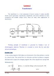
Department of Electrical Engineering 

EE 303: 

Electronic Circuits II 

Laboratory Manual 

July 2008 

1

KING FAHD UNIVERSITY OF PETROLEUM AND MINERALS 

DEPARTMENT OF ELECTRICAL ENGINEERING 

Electronic Circuits II – EE303 

Tutorial # 1 

Net Listing and Simulation Analysis Using SPICE 

OBJECTIVES 

1. Describe net listing and simulation analysis using SPICE. 

2. Introduce diodes and transistors’ models used in SPICE. 

3. Explain additional SPICE commands and test new circuits. 

4. Test new circuits using default and commercial parameters. 

INTRODUCTION 

Currently, one of the more widely used general purpose circuit simulation program for 

industrial and academic computer systems is SPICE. As you know SPICE can be used to 

simulate circuits containing resistors, capacitors, inductors, mutual inductors, 

independent and dependent voltage and current sources, and basic semiconductor 

devices. In EE 203 students were using Schematic Editor of SPICE to draw circuits and 

then run simulation analysis. In fact, drawing circuits and ensuring correct 

interconnections may be time consuming. Alternatively, circuits can be described in 

SPICE by specifying their various components and their terminal connections (net 

listing). A typical SPICE input file format is as follows: 

Notes: 

TITLE STATEMENT 

CIRCUIT ELEMENTS: 

Power Supplies / Signal Sources 

Circuit description/Element Descriptions 

Model Statement 

* Comments 

CONTROL COMMANDS: 

Analysis Requests 

Output Requests 

* Comments 

.END 

1. The first line must be a title line which is usually reflects the file contents. It 

cannot be omitted. 

2. The last line must be the .END statement. 

3. You can insert comment lines starting with "*". 

2

4. You can use upper or lower case letters. 

5. The following subsections explain how to describe elements and use the 

control commands. 

CIRCUITS ELEMENTS 

1. The general format for describing independent voltage source is 

Vname N+ N- [DC value] [AC Magn phase] or [SIN V 0 V a freq td df 

phase] 

Where 

The voltage source must start with letter V. 

N+ and N- are the positive and negative nodes of the source, respectively. 

Sources can be assigned values for dc analysis [DC value], ac analysis [AC 

magnitude phase], or transient analysis [SIN]. 

The ac phase angle is in degrees. 

The parameters of the sin are given in this order: dc offset, amplitude, frequency, 

delay, damping factor, phase, respectively. In most cases there is no need to 

specify td, df, and phase but rather leave SPICE use their default values of 

zeroes. 

Other the transient signal generators such as PULSE and PWL are introduced in 

Experiment 3. 

2. An independent current source can be described similarly but using Iname to replace 

Vname. But note that current flows from a positive node to the negative node. 

3. Various dependent sources are defined when needed in Experiments 3 and 4. 

4. Passive elements are described by element statements that specify the type-name and 

terminal connections as follows: 

Rname N1 N2 value 

Cname N1 N2 value 

Lname N1 N2 value 

5. Semiconductor devices such as diodes, MOSFETs and BJTs are described by two 

statements. In addition to an element statement, a model statement is required. SPICE 

allows varying degrees of circuit element model complexity. In this tutorial we intend to 

provide basic default model descriptions and more complex model descriptions. 

Examples will be used to illustrate the differences between the results obtained using 

hand calculations, default device models and complex device models. By the end of this 

tutorial we expect that the student will get an appreciation of the advantages of using 

SPICE complex models. The following subsections briefly described element and model 

statements for basic semiconductor devices. 

3

Diode Models 

The diode element model is given in Figure 1. The element statement format is given by 

Dname NA NC MNAME [AREA] 

NA 

MNAME 

NC 

I D 

The associated model statement is 

Figure 1: Junction Diode. 

.MODEL MNAME D [PNAME1=PVAL1 PNAME2=PVAL2…] 

The anode of the diode is connected to NA; the cathode to NC. MNAME is an 

alphanumeric model designation for the device. Detailed model parameters are provided 

in Table 1. 

Bipolar Junction Transistor 

The npn and pnp transistor element models are shown in Figure 2. The element statement 

format is 

Qname NC NB NE MNAME [AREA] 

NC 

NC 

NB 

NB 

NE 

NPN 

Figure 2: BJT types. 

NE 

PNP 

The associated model statements is 

or 

.MODEL MNAME npn [PNAME1=PVAL1 PNAME2=PVAL2…] 

.MODEL MNAME pnp[PNAME1=PVAL1 PNAME2=PVAL2…] 

4

Detailed model parameters are provided in Table 2. 

MOS Field Effect Transistor 

The n-channel and p-channel MOSFET element models are given in Figure 3. The 

element statement format is 

Mname ND NG NS NB MNAME W=VALW L=VALL 

ND 

ND 

NG 

NB 

NG 

NB 

NS 

NS 

5 

NMOS 

PMOS 

Figure 3: MOSFET types. 

The associated model statements is for N-channel 

.MODEL MNAME NMOS [PNAME1=PVAL1 PNAME2=PVAL2…] 

and for P-channel 

.MODEL MNAME PMOS[PNAME1=PVAL1 PNAME2=PVAL2…] 

Detailed model parameters are provided in Table 3. Note that the default values for the 

gate length, VALL, and the gate width, VALW, are 1cm. Obviously, these are not 

realistic values; however, the model uses the ratio of VALL and VALW rather than the 

individual values in its calculations. 

CONTROL COMMANDS 

.OP 

The inclusion of the statement .OP makes SPICE perform DC analysis to find the 

operating point of the circuit. 

.AC Sweep-mode NP START STOP 

The .AC control statement is used to perform ac analysis on a circuit and provide 

data for frequency response plotting. 

Where Sweep-mode is one of the keywords that’s indicates the frequency 

variation by decade (DEC), by octave (OCT), or linearly (LIN). 

NP is the number of points per sweep-mode; 

FSTART is the starting frequency. FSTART cannot be zero.

FSTOP is the final or ending frequency. 

.DC SOURCE_NAME START_VAL STOP-VAL INCREMENT_VAL 

The .DC control statement specifies the values that will be used for dc sweep or 

dc analysis. 

Where SOURCE_NAME is the name of an independent voltage or current 

source. START_VAL, STOP_VAL and INCREMENT_VAL represent the 

starting, ending, and increment values of the source, respectively. 

.TRAN TSTEP TSTOP 

.TRAN makes SPICE perform a time domain transient analysis of the circuit 

TSTEP is the time increment used for plotting and/or printing results of the 

analysis. 

TSTOP is the time of the last transient analysis. 

.PRINT ANALYSISTYPE OV 

The inclusion of the .PRINT statement makes SPICE perform a print of a 

specified output variable resulting from a specified type of analysis. 

where ANALYSISTYPE is the type of analysis performed from which the output 

variable OV is obtained. 

.PROBE 

Probe in SPICE is the graphics postprocessor that calculates and displays results 

of a simulation. In effect, Probe functions as a “software” oscilloscope, calculator, 

and spectrum analyzer. Arithmetic operations on output variables are allowed in 

SPICE Probe. Always include .Probe statement to help in plotting your results. 

WRITING AND RUNING THE PROGRAME 

‣ Create an input file (source file) or Circuit description file for SPICE. 

You can run SPICE by going to programs→SPICE Student→SPICE AD 

Student from the start Menu. Next, we have to create text file that describes our 

circuit and the simulation protocol. Create a new text file (File→New→Text 

File) with any editor, such as Microsoft editor, Word perfect, Notepad under 

windows, etc. and immediately save it (File Save As…) with the extension .cir 

(example:circuit1.cir). Now you must open the file (File→Open, and change the 

“Types of Files” to “Circuit Files”) before SPICE recognize it as a valid circuit 

description file. 

6

‣ Run the program 

Once you are in SPICE, pull down the File menu at the top of the screen and 

select "Open ". The system prompts you for the name of the file. Type in the file 

name of the circuit you have created before. As an example: c:\users\Circuit1.cir. 

Run the simulation (Simulation→Run). A window will appear telling you that 

Spice program is running, or that the simulation has been completed successfully, 

or that errors were detected. Click on the "OK" button. 

‣ Look at the output file and print the results 

The output file always generated by SPICE is the text file that has the file type 

“OUT”. Let’s say you submit a data file to SPICE named “CIRCUIT1.CIR”, it 

will create an output file named “CIRCUIT1.OUT”. This output file is created 

even if your run is unsuccessful due to input errors. The cause of failure is 

reported in the *.OUT file, so this is a good place to start looking when you need 

to debug your simulation model. 

An easier way of plotting the results is to use (Add about using probe to see 

results) 

XXXXXXXXXXXXXXXXXXXXXXXXXXXXXXXXXXXXXXXXXXXXX 










XXXXXXXXXXXXXXXXXXXXXXXXXX 

7

GENERAL EXAMPLES 

At this stage you are requested to write and run the following three programs, obtain the 

results from SPICE simulation. Before start writing the program label all nodes with the 

common node (ground) always has number "0". 

1. The input file of the circuit of 

Figure 4 can be as follows: 

PWRSUP.CIR 

* Sin input with 100V amplitude 

*and 50Hz frequency 

VAC 10 0 SIN(0 100 50) 

D 10 11 MODR 

* default model 

.MODEL MODR D 

RS 11 12 2 

CF 12 0 40U 

RL 12 0 1K 

.TRAN 1M 40M 

*Who many cycle will be 

plotted? 

.PLOT TRAN V(12) 

.PROBE V(12) 

.END 

R S 

10 D 11 12 

V AC 

C F 

R L 

0 

Figure 4: Circuit for example 1. 

FREQUNCY RESPONSE EXAMPLES 

The main objective of the following two examples is to understand different frequency 

bands in the amplifier frequency response where a typical frequency response of a 

capacitively coupled transistor amplifiers is shown in Figure 5. At low frequency band 

the coupling and bypass capacitors are in effect. Whereas, at high frequency band the 

transistor internal capacitances are in effect. 

8

|Av(jω)| 

[dB] 

A m 

F L (jω) 

F H (jω) 

Midband 

region 

w P1 

w Z2 

w P2 w P3 w P4 

w H 

w L 

Figure 5: Typical amplifier’s frequency response 

w 

[log scale] 

2. The input file of the circuit of Figure 6 is: 

MOSFET CS Amplifier 

vsig 1 0 ac 1 sin(0 5m 100k) 

VDD 6 0 DC 5V 

Rsig 1 2 1K 

C1 2 3 0.15uF 

Mamp 4 3 5 5 M2N4351 W=100U L=100U 

.MODEL M2N4351 NMOS (LEVEL=1 +VTO=2.1 

KP=1.12M GAMMA=2.6 

+ PHI=.75 LAMBDA=2.49M RD=14 RS=14 + 

IS=15F PB=.8 MJ=.46 

+ CBD=7.95P CBS=9.54P CGSO=11.7N 

+ CGDO=9.75N CGBO=16N) 

R1 3 0 400K 

R2 6 3 100K 

RS 5 0 1.3K 

Cs 5 0 10uF 

RD 6 4 4.3K 

C2 4 7 0.15uF 

Rl 7 0 100K 

.ac dec 100 10 40meg 

.print ac v(7) 

* Will print the frequency response 

.tran 0.01u 20u 

.print tran v(7) 

*Will print the output wave form at frequency 100kHz 

.END 

Rsig 

1k 

vsig 

C1 

0.15 

100k 

300k 

R2 

R1 

RD 

RS 

4.3k 

M 

+VDD=5V 

C2 

0.15 

CS 

1.3k 10 

RL 

vo 

100k 


Requirements: 

1. Label the nodes according to the input file. 

2. Run the program using default mode first. 

3. Find A M 

4. Determine f H , and f L where A M reduces to 

0.707A M 

5. Then, add the given practical model and run the 

program. 

6. Observe the differences. 

9

3. The input file of the circuit of Figure 7 is: 

BJT CE Amplifier 

vsig 1 0 ac 1 sin(0 5m 100k) 

VCC 6 0 DC 5V 

Rsig 1 2 1K 

C1 2 3 1uF 

.op 

Qamp 4 3 5 Q2N3904 

.model Q2N3904 NPN(Is=6.734f 

+Xti=3 Eg=1.11 +Vaf=74.03 Bf=416.4 

Ne=1.259 +Ise=6.734f Ikf=66.78m 

Xtb=1.5 +Br=.7371 Nc=2 Isc=0 Ikr=0 

+Rc=1 Cjc=3.638p Mjc=.3085 +Vjc=.75 

Fc=.5 Cje=4.493p +Mje=.2593 Vje=.75 

Tr=239.5n +Tf=301.2p Itf=.4 Vtf=4 Xtf=2 

+Rb=10) 

R1 3 0 400K 

R2 6 3 100K 

RS 5 0 1.3K 

Cs 5 0 10uF 

RD 6 4 4.3K 

C2 4 7 0.15uF 

Rl 7 0 100K 

.ac dec 100 10 40meg 

.print ac v(7) 

.tran 0.01u 20u 

.print tran v(7) 

.END 

5V 

+ 

- 

R S 

Vs 

Vcc 

1k 

C 1 

1 

R B1 

30k 

R C 

4.3k 

R B2 10k 

R E 1.3k 

C E 


Requirements: 

1. Label the nodes according to the input file. 

2. Run the program using default mode first. 

3. Find A M 

4. Determine f H , and f L where A M reduces to 0.707A M 

5. Then, add the given practical model and run the program. 

6. Observe the differences. 

Q1 

C 2 

1 

47 

R L 

V out 

100k 

ASSIGNMENT 

Consider the BJT amplifier circuit shown in Figure 8 and perform the following: 

1. Using the default parameters of the BJT, write a SPICE program to plot the gainfrequency 

characteristic. From the SPICE output file, calculate the medium frequency 

gain and the upper and lower 3dB points. 

2. Repeat step 2 using the practical model given below. 

3. Comment on your results. 

10

Spice Transistor Model 

.model Q2N3904 NPN(Is=6.734f Xti=3 Eg=1.11 Vaf=74.03 Bf=416.4 Ne=1.259 

+ Ise=6.734f Ikf=66.78m Xtb=1.5 Br=.7371 Nc=2 Isc=0 Ikr=0 Rc=1 

+ Cjc=3.638p Mjc=.3085 Vjc=.75 Fc=.5 Cje=4.493p Mje=.2593 Vje=.75 

+ Tr=239.5n Tf=301.2p Itf=.4 Vtf=4 Xtf=2 Rb=10) 

+ 

5V 

- 

R Sig 

Vsig 

Vcc 

1k 

C 1 

1 

R B1 

R C1 4.3k 

30k 

C 2 

Q1 

1 

2N3904 

R B2 10k 

R E1 1.3k 

C E 

R B3 

R B4 

47 

30k 

10k 

4.3k 

R E2 

2N3904 

1 

C 3 

1.3k 100k R L 

V out 

Figure 8: Circuit for assignment. 

11

TABLE 1: DETAILED DIODE MODEL PARAMETERS 

Model Parameters Default Units 

IS saturation current 1E-14 A 

N emission coefficient 1 

RS parasitic resistance 0 ohm 

CJO zero-bias pn capacitance 0 farad 

VJ pn potential 1 volt 

M pn grading coefficient 0.5 

FC forward-bias depletion capacitance coefficient 0.5 

TT transit time 0 S 

BV reverse breakdown voltage infinite volts 

IBV reverse breakdown current 1E-10 A 

EG bandgap voltage (barrier height) 1.11 eV 

XTI IS temperature exponent 3 

KF flicker noise coefficient 0 

AF flicker noise exponent 1 

12

TABLE 2: DETAILED BJT MODEL PARAMETERS 

Model Parameters Default Units 

IS pn saturation current lE-16 A 

BF ideal maximum forward beta 100 

NF forward current emission coefficient 1 

VAF (VA) forward Early voltage infinite V 

IKF (IK) corner for fwd beta high-cur roll off infinite A 

ISE (C2) base-emitter leakage saturation current 0 A 

NE base-emitter leakage emission coefficient 1.5 

BR ideal maximum reverse beta 1 

NR reverse current emission coefficient 1 

VAR (VB) reverse Early voltage infinite V 

IKR corner for rev beta hi-cur roll off infinite A 

ISC (C4) base-collector leakage saturation current 0 A 

NC base-collector leakage emission coefficient 2.0 

RB zero-bias (maximum) base resistance 0 ohm 

RBM minimum base resistance RB ohm 

RE emitter ohmic resistance 0 ohm 

RC collector ohmic resistance 0 ohm 

CJE base-emitter zero-bias pn capacitance 0 F 

VJE (PE) base-emitter built-in potential 0.75 V 

MJE (ME) base-emitter pn grading factor 0.33 

CJC base-collector zero-bias pn capacitance 0 F 

VJC (PC) base-collector built-in potential 0.75 V 

MJC (MC) base-collector pn grading factor 0.33 

XCJC fraction of C bc connected into R b 1 

CJS (CCS) collector-substrate zero-bias pn capacitance 0 F 

VJS (PS) collector-substrate built-in potential 0.75 

MJS (MS) collector-substrate pn grading factor 0 

FC forward-bias depletion capacitor coefficient 0.5 

TF ideal forward transit time 0 s 

XTF transit time bias dependence coefficient 0 

VTF transit time dependency on Vbc infinite V 

ITF transit time dependency on Ic 0 A 

PTF excess phase @ 1/ (2πTF) Hz 0 °C 

TR ideal reverse transit time 0 s 

EG bandgap voltage (barrier height) 1.11 eV 

XTB forward and reverse beta temp coefficient 0 

XTI(PT) IS temperature effect exponent 3 



13

TABLE 3: DETAILED MOSFET MODEL PARAMETERS 

Model Description Default Units 

LEVEL model type(l, 2, or 3) 1 

L channel length DEFL meter 

W channel width DEFW meter 

LD lateral diffusion (length) 0 meter 

WD lateral diffusion (width) 0 meter 

VTO zero-bias threshold voltage 0 volt 

KP transconductance 2E-5 A/V 2 

GAMMA bulk threshold parameter 0 volt l/2 

PHI surface potential 0.6 volt 

LAMBDA channel-length. modulation (LEVEL 1 or 2) 0 volt -1 

RD drain ohmic resistance 0 ohm 

RS source ohmic resistance 0 ohm 

RG gate ohmic resistance 0 ohm 

RB bulk ohmic resistance 0 ohm 

RDS drain-source shunt resistance infinite ohms 

RSH drain-source diff. sheet res. 0 ohm/sq. 

IS bulk pn saturation current 1E-14 A 

JS bulk pn sat. current/area 0 A/m 2 

PB bulk pn potential 0.8 volt 

CBD bulk-drain zero-bias pn cap. 0 farad 

CBS bulk-source zero-bias pn cap. 0 farad 

CJ bulk pn zero-bias bot. cap./area 0 F/m 2 

CJSW bulk pn zero-bias perimeter cap./length 0 F/m 

MJ bulk pn bottom grading coefficient 0.5 

MJSW bulk pn sidewall grading coefficient 0.33 

FC bulk pn forward bias capacitance coefficient 0.5 

CGSO gate-source overlap capacitance/channel width 0 F/m 

CGDO gate-drain overlap capacitance/channel width 0 F/m 

CGBO gate-bulk overlap capacitance/channel length 0 F/m 

NSUB substrate doping density 0 cm -3 

NSS surface state density 0 cm -2 

NFS fast surface state density 0 cm -2 

TOX oxide thickness infinite meter 

TPG gate material type; +1 = opposite of substrate; +1 

-1 = same as substrate; 0 = aluminum 

XJ metallurgical junction depth 0 meter 

UO surface mobility 600 cm 2 /Vs 

UCRIT mobility degradation critical field (LEYEL=2) IE4 V/cm 

UEXP mobility degradation exponent (LEVEL=2) 0 

UTRA (not used) mobility degradation transverse field coefficient 

VMAX maximum drift velocity 0 m/s 

NEFF channel charge coefficient (LEVEL=2) 1 

XQC fraction of channel charge attributed to drain 1 

DELTA width effect on threshold 0 

THETA mobility modulation (LEVEL=3) 0 volt -1 

ETA static feedback (LEVEL=3) 0 

KAPPA saturation field factor (LEVEL=3) 0.2 



14




Experiment # 1 

Frequency Response of the Common Source Amplifier 

OBJECTIVES 

1. To measure the frequency response of common source (CS) amplifier. 

2. To determine the useful bandwidth of the CS amplifier by finding the midband 

frequency gain (A M ), the low and high 3dB corner frequencies. 

3. To investigate the effect of load resistance on the frequency response. 

4. To study the effect of the bypass capacitor on the frequency response. 

A typical CS amplifier is shown in Figure 1. 

BACKGROUND 

+V DD =5V 

100k 

R 2 

R D 

4.3k 

C 2 

v o 

R sig 

C 1 

C S 

R L 

1k 

v sig 

0.15 

300k 

R 1 

R S 

2N4351 

0.15 

1.3k 10 

100k 

15 

Figure 1: A typical common source amplifier 

As you have studied in your lectures small signal ac analysis can be used to shown that: 

1. The midband frequency gain (A M ) is given by: 

vo RG 

' 

AM 

gmRL 

(1) 

v R R 

sig sig G 

Where RG 

R1|| 

R2 

and R L 

RL || RD 

2. The low and high -3dB pole frequencies can be estimated as: 

3 1 1 1 1 

wL 

 

i1 

R 1 

iSCi C1( RSig RG ) C2( RL RD 

) 

CS( RS 

|| ) 

g 

m 

(2)

1 1 

wH 

 

R C C C gmR R R C C R R 

16 

 

' 

iS i 

[ 

GS 

 

GD 

(1 

L)] sig 

// 

G 

( 

GD 

 

DB 

) 

D 

// 

L 

3. Also, it can be shown that when Cs is removed the gain will decrease to: 

' 

Rg 

gmRL 

AM 

(4) 

R R 1 

g R 

sig 

g 

m 

s 

4. The value of ω L will decrease whereas that of ω H will increase. 

1 1 

wL 

 

(5) 

C1( RS RG ) C2( RL RD 

) 

1 

wH 

 

(6) 

' 

' 

Rth 

R 

g 

' mR R 

L th 

R R 

s 

L s 

CGS ( ) CGD ( Rth R ) C ( ) 

L 

DB 

1 gmRs 1 gmRs 1 

gmRs 

In fact, the amplifier bandwidth (BW) is defined as the difference between 

f H 

w H 

/( 2 

) and f L 

w L 

/( 2 

) and since, usually f 

L 

f 

H 

, BW f H 

. Normally, the 

amplifier is designed so that its bandwidth coincides with the spectrum of the signals that 

it is required to amplify. Otherwise, signal distortion will occur. 

Finally, a figure-of-merit for the amplifier is its gain-bandwidth product, which is defined 

as GB= A BW. It will be seen that in amplifier design there is usually trade-off between 

M 

gain and bandwidth. 

EQUIPMENTS & COMPONENTS 

1. Signal generator, Bread Board, Digital Multi-Meter, and Digital Oscilloscope. 

2. DC supply V DD =5V from the Board 

3. MOSFET 2N4351. 

4. Resistors: R sig = 1kΩ, R 1 = 300kΩ, R 2 = 100kΩ, R D = 4.3kΩ, R S = 1.3kΩ, 

R L =100kΩ or 10kΩ. 

5. Capacitors: C 1 = 0.15μF, C 2 = 0.15μF, C S = 10μF. 

PRELAB WORK 

Students must perform the hand calculations and SPICE before the lab. 

Hand Calculation: 

1. With C S , calculate A M , f 

L 

, f 

H 

, BW, and GB for R L =100kΩ and R L =10kΩ assuming 

g m =1.04mA/V. Try to deduce the trade-of between gain and bandwidth from these 

results. 

2. From the results obtained in step 1, try to deduce the effect of R L on the A M and the 

bandwidth? 

3. Without C s , calculate A M , f 

L 

, f 

H 

, and BW when R L =100kΩ. 

4. From the results obtained in step 1 and 3, try to deduce the effect of C s on the A M and 

the BW? 

5. Record your results in Table II. 

(3)

SPICE Simulation: 

SPICE simulations can be used to verify the hand calculations. In practice, howevere, 

stray and bread board capacitances will affect high frequency pole significantly. So, to 

compare your experimental results for fH 

with SPICE you need to add parasitic 

capacitances in your SPICE file. For example, use three parastic capacitances between 

each two terminals of the transistors. 

6. Use PISCE program developed in the pervious SPICE tutorial to generate three 

output files for the cases: (a) With C s and R L =100kΩ (b) With C s and R L =10kΩ (c) 

Without C s and R L =100kΩ. Use no parastic capacitances. 

7. Determine A M , f 

L 

, f 

H 

, BW, and GB for each case. 

8. Record your results in Table II. 

9. Repeat steps 6 and 7 but using parastic capacitances of about 20pF. 

10. Record your results in Table III. 

EXPERIMENTAL WORK 

See pin configurations of MOSFET 2N4351 in the data sheet given in the Appendix at the 

end of the manual. 

1. Construct the circuit shown in Figure 1 with the capacitor C S and R L =100kΩ. Apply a 

small ac signal v sig with a frequency in the midband (about 10kHz). Keep increasing 

the amplitude and make sure by monitoring the oscilloscope that the output voltage is 

not distorted. Using v sig that results in maximum undistorted output (approximately 

20mVp-p), in the remaining steps. 

(a) Measure the output amplitude in midband (the output should be constant over 

wide range of frequencies). Calculate A M by dividing the amplitude of the output 

signal by that of the input signal. 

Notes: 

i. You may use Table I to record your readings. 

ii. Keep monitoring the input value during measurement since it may 

vary. Always adjust it to 20mVp-p in order to get correct data. 

iii. Note that at low-frequency the output signal will be noisy, to reduce 

this effect use the average function on the oscilloscope by pressing the 

acquire knob, do this for frequencies above 1MHz also. 

(b) Change the input frequency gradually from 10kHz to about 20Hz. At each 

frequency measure the small signal voltage gain. Give a special attention to the 

frequency where gain reduces to A 

M 

/ 2 . 

(c) Now set the frequency back to 10kHz and gradually increase the frequency up to 

2MHz and measure the small signal voltage gain at each step. Again give a 

special attention to the frequency where A M reduces to A / 2 

2. Plot this set of data on the provided graph sheet (Figure 2). 

M 

17

3. Calculate the A M , f 

L 

, 

characteristics. 

f 

H 

, BW and GB from your measured gain-frequency 

4. Change R L to 10kΩ repeat step 1 through 3. 

5. Remove Cs and change R L back to 100kΩ repeat step 1 through 3. 

6. Insert your experimental results into Table III. 

7. Compare your hand calculations, SPICE simulations and experimental measurements. 


18

Table I: Measurement results 

With C s and R L =100kΩ With C s and R L =1kΩ Without C s and R L =100kΩ 

f Gain Gain in 

dB 


dB 


dB 

19

This page to be submitted with the report 

Table II: Summary of hand calculations, SPICE simulations. 

Hand Calculation 

SPICE Simulation 

Parameter 

Without C S 

With C S 

With C S 

Without C S 

With C S 

With C S 

R L=100k 

R L=100K 

R L=1K 

R L=100k 

R L=100K 

R L=1K 

A M 

f 

L 

f 

H 

BW 

GB= 

AM 

BW 

Table III: Summary of SPICE simulation including parasitic capacitances and experimental results. 

SPICE Simulation 

With parasitic capacitances 

Experimental Result 

Parameter 

Without C S 

With C S 

With C S 

Without C S 

With C S 

With C S 

R L=100k 

R L=100K 

R L=1K 

R L=100k 

R L=100K 

R L=1K 

A M 

f 

L 

f 

H 

BW 

GB= 

AM 

BW 

20


Figure 2: Frequency Response of CS amplifier 

21





Frequency response of multistage transistor amplifiers 

OBJECTIVE 

1. To measure the frequency response of common emitter (CE) amplifier. 

2. To study the effect of the load resistance R L on the frequency response of the 

CE amplifier. 

3. To explore some advantages of using multistage amplifier Common Emitter- 

Common-Collector amplifier. 

BACKGROUND 

A typical common emitter (CE) amplifier is shown in Figure 1. 

5V 

+ 

- 

Vcc 

R B1 

30k 

R C1 

4.3k 

C 2 

C 1 

Q1 

1 

V out 

R Sig 

1k 

1 

R L 

100k 

Vsig 

R B2 10k 

R E1 1.3k 

C E 

47 

Figure 1: Common Emitter amplifier 

As you have studied in your lectures, it can be shown using small signal ac analysis that: 

1. The midband frequency A M gain is given by: 

vo 

vbe 

vo 

Rin 

' 

A 

M 

g 

mRL 

(1) 

v v v R R 

sig 

sig 

be 

sig 

in 

22

where R R 1 

// R 2 

// r and ' 

in B B 1 

RL 

RL 

// RC1 

2. The low frequency pole can be approximated by the pole due to the capacitor 

assoiciated with the lowest resistance namely C E : 

1 

wL 

 

(2) 

r 

RS 

// RB 

1 

// RB2 

CE 

( RE1 

// 

) 

1 

 

3. The high frequency pole can be approximated by the pole due to input capacitance 

which becomes significantly large because of miller’s capacitance C eq = C ' 

(1 g R m 

) 

1 eq in s 1 

m L in s 

1 L 

: 

1 

1 

wH 

 

(3) 

' 

[ C C ] R // R C g R ( R // R ) 

' 

Where g m RL 

represents the voltage gain between the two terminals of C μ1 (i.e. the gain 

between the collector and base of Q1). Since R L is connected at the collector of Q1, 

changing its value will directly alter both A M and ω H . In order to maintain almost constant 

gain and hence constant bandwidth a buffer stage or common-collector (CC) amplifier 

can be used to isolate the load from the basic CE amplifier or C μ1 as shown in Figure 2. 

Now the input resistance of the CC amplifier (R in2 ) will act as the new load derived by 

the collector of Q1. The input resistance of Q2 is slightly dependent on R L and hence 

changing R L will lead to small variation in the gain and ω H . In other words, since the CC 

amplifier has a relatively small output resistance which can derive various loads while 

maintaining almost constant gain. Keeping the gain almost constant will also results in 

constant bandwidth. Also, note that since CC amplifier has usually much larger 

bandwidth than that of the CE amplifier, the overall bandwidth of the multistage 

amplifier will mainly be decided by the poles of CE amplifier. 

+ 

5V 

- 

R Sig 

Vsig 

Vcc 

1k 

C 1 

1 

R B1 

R C1 4.3k 

30k 

C 2 

Q1 

1 

2N3904 

R B2 10k 

R E1 1.3k 

C E 

R B3 

R B4 

47 

30k 

10k 

4.3k 

R E2 

2N3904 

1 

C 3 

1.3k 100k R L 

V out 

Figure 2: Common Emitter amplifier with Buffer 

With the buffer connected the midband the various parameters become: 

v 

o 

Rin 

'' 

1. A M 

g 

mRL 

ABuffer 

(4) 

v R R 

sig 

sig 

in 

23

'' 

Where RL 

RC 

1 

// Rin2 

RC 

1 

// RB3 

// RB4 

//[ r 2 

( RL 

// RE2)(1 

)] 

and 

RL 

// RE2 

(1 ) 

A 

Buffer 

 

(5) 

r 

2 

RL 

// RE2 

(1 ) 

2. Note that C 3 is associated with relatively small resistance and hence may significantly 

contribute to value of the low frequency pole particularly when R L is small: 

1 

1 

wL 

 

 

(6) 

r 

RS 

// RB 

1 

// RB2 

r 

2 

RC1 

// RB 

1 

// RB2 

CE 

( RE1 // 

) C3[( 

RE2 

// 

) RL 

] 

1 

 

1 

 

3. The high frequency pole can be expressed as: 

1 

1 

wH 

 

(7) 

'' 

'' 

[ C C (1 g R )] R // R C g R ( R // R ) 

1 1 

m L in s 1 

m L in s 

' 

It can be seen that unlike R 

L 

, the value of 

values. 

'' 

R 

L 

will be almost constant for different load 


1. Digital Oscilloscope, Bread Board, Digital Multi-Meter, Signal generator. 

2. DC supply V cc =5V from the Board. 

3. Two BJT 2N3904. 

4. Resistors: R sig =1k,R B1 =R B2 =30k, R B3 =R B4 =10k, R C1 =4.3k,R E1 =R E2 =1.3k, 

R L =100k and 1K. 

5. Capacitors: C E =47μF,C 1 =C 2 =C 3 =1μF. 

PRELAB WORK 

Students must perform the following calculations and SPICE before the lab. 


1. Given that g m1 =g m2 =16.9mA/V and r π1 = r π2 =7.2kΩ, complete the Table I. 

R 

' 

'' 

L 

R 

L 

R 

L 

1 kΩ 

100 kΩ 

% Change 

A Buffer 

2. For the two amplifier circuits shown in Figure 1 and Figure 2 calculate A M , f 

L 

, f , H 

BW and GB required to complete Table II. 


3. Use the programs developed in the pervious SPICE tutorial to generate the required 

outputs for Figure 1 and Figure 2 to determine A M , f 

L 

, f 

H 

, BW and GB to complete 

Table II. For the SPICE analysis use the frequency range 10Hz to 8MHz. Use the BJT 

model given in the tutorial. 

24

4. Use three parastic capacitances of about 10pF between each two terminals of the 

transistors. Repeat step 3 and determine f H 

, BW and GB and record your results in 

Table II. 


See pin configurations of BJT 2N3904 in the data sheet given in the Appendix at the end 

of the manual. 

1. Construct the circuit shown in Figure 1. Apply a small ac signal v sig and frequency in 

the midband about 10kHz. Keep increasing the amplitude and make sure by 

monitoring the output on oscilloscope that the output voltage is not distorted. 

Calculate A M. Use the corresponding value of v sig in the remaining steps. 

2. Reduce the input frequency from 10kHz gradually to find f 

L 

. 

3. Go back with frequency to 10kHz and increase it gradually to find f H 

. 

4. Calculate BW and GB from your measured gain-frequency characteristic. 

5. Repeat steps 1 through 4 when R L is changed to 1kΩ. 

6. Construct the circuit shown in Figure 2 with R L =100kΩ. 

7. Repeat steps 1 through 4 for Figure 2. 

8. Repeat steps 1 through 4 for Figure 2 when R L is changed to 1kΩ. 

9. Insert your experimental results into Table IV. 



25


Table II: Summary of hand calculations 

Figure 1 Figure 2 

Parameter 

R L =1 kΩ 

R L =100 kΩ 

% 

Change R L =1 kΩ R L =100 kΩ 

% 

Change 

A M 

f 

L 

f 

H 

BW 

GB= 

AM 

BW 

Table III: Summary of SPICE simulations 


Parameter 

R L =1 kΩ 

R L =100 kΩ 

% 


% 

Change 

A M 

f 

L 

f 

H 

f 

H 

(with parasitic 

capacitances) 

BW 

BW (with parasitic 

capacitances) 

GB= 

AM 

BW 

GB (with parasitic 

capacitances) 

26


Table IV: Summary of Experimental results 


Parameter 

R L =1 kΩ 

R L =100 kΩ 

% 


% 

Change 

A M 

f 

L 

f 

H 

BW 

GB= 

AM 

BW 

27





Linear Applications of Operational Amplifier 

OBJECTIVE 

1. To measure the characteristics of several linear circuits based on the operational 

amplifier namely inverting amplifier, inverting summer, inverting integrator, 

inverting differentiator and differential amplifier. 

2. Learn factors involved in circuit design using op amps. 

3. To design circuits to implement simple linear functions. 

BACKGROUND 

This section provides brief discussion of the main characteristics of the op amp based 

circuits shown in Figure 1: 

Unity-gain Buffer: 

It has a voltage gain, input resistance and output resistance of A v / v 1, R and 

R 

o 

0 , respectively. It does not take any input current and can drive any desired load 

resistance without loss of signal voltage. Thus, it used to provide excellent impedancelevel 

transformation while maintaining signal voltage level. 

Inverting Amplifier: 

It has a voltage gain, input resistance and output resistance of A v / v R / R 

v 

 

o i 

 

2 1, 

R i 

R 1 

and R 

o 

0 , respectively. The minus sign means a 180 o phase shift between the 

output and input signals 

Summing Amplifier: 

The output voltage can be expresses as v o 

[( R3 / R1 

) v1 

( R3 

/ R2 

) v2] 

. 

It can be seen that the scale factors for the two inputs can be independently adjusted by 

proper choice of R 2 and R 1 . Also, more inputs can be added simply by connecting them 

same way as v 1 and v 2 . Hence, it can be used as a simple digital-to-analog converter. 

Inverting Integrator: 

v 

o 

i 

i 

28

1 

The output voltage in time domain can be expresses as v 

o( t) 

vi 

( ) d 

vi 

( to) 

RC 

This means that the output voltage at time t is given by the initial capacitor voltage plus 

the integral of the input signal from start of integration interval, here, t=0. Note that dc 

gain is infinity which means any small dc component of v i (t) results in output. In 

practice, the op amp will saturates at a voltage close to positive or negative supply 

depending on input voltage polarity. 

Differentiator: 

dvi 

( t) 

The output voltage in time domain can be expresses as vo 

( t) 

RC 

dt 

This means that the output is scaled version of derivative of input voltage. The 

differentiator is noise magnifier (i.e. spikes may be produced at output due to sharp 

changing in v i (t)). 

Difference Amplifier: 

This circuit amplifies difference between two input signals. The output voltage can be 

expresses as R / R )( v v ) ( R / R )( v ) . 

v o 

( 

2 1 1 2 2 1 2 

v1 

Voltage to Current Converter: 

Such a converter is capable of producing a current into a load that is independent of the 

load value and also proportional to the input voltage. It can be shown for the simple 

voltage to current converter given in Figure 1 that I out =V i /R regardless of the value of Z L . 

Can you prove that? 



2. DC power Supplies of 10V and -10V from the Board. 

3. Op amps 741. 

4. Resistors: 1kΩ, 2kΩ, 5kΩ, 10kΩ, 100kΩ. 

5. Capacitors: 1.5nF, 0.1μF. 

t 

t 

o 

29

Function 

Unity-gain Buffer 

CIRCUIT 

2 

3 

4 

+ 

741 

- 

+15V 

7 

-15V 

R 2 =5k 

6 

V out 

Inverting Amplifier 

R 1 =1k 

2 

3 

7 

- 

741 

+ 

+15V 

4 

-15V 

6 

V out 

R 1 =1k 

R 3 =2k 

Summing Amplifier 

(Adder) 

R 2 =1k 

2 

3 

7 

- 

741 

+ 

+15V 

4 

-15V 

6 

V out 

1500pF 

Inverting Integrator 

100k 

2 

3 

7 

- 

741 

+ 

+15V 

4 

-15V 

6 

V out 

30

10k 

Differentiator 

1500pF 

2 

3 

7 

- 

741 

+ 

+15V 

4 

-15V 

6 

V out 

R 2 =2k 

Difference Amplifier 

R 1 =1k 

R 1 =1k 

+15V 

2 

- 

7 

741 

+ 

3 

4 

R 2 =2k -15V 

6 

V out 

R X =5k 

R X =5k 

2 

+15V 

7 

- 

741 

3 

+ 

4 

Voltage to Current Converter R=10k 

-15V 

6 

V out 

1k or 2k 

Z L 

I out 

R=10k 

Figure 1: Basic applications based on op amp. 

PRELAB WORK 

Students must perform the following calculations and SPICE before coming to the 

lab. 

During design phase, use typical values of resistors and capacitors from the list provided 

in the Appendix of this manual. 

31


1. For the different configurations shown in Figure 1, perform an approximate hand 

calculation assuming that the operational amplifier is ideal. In each case sketch the 

expected output waveform in Table I. Assume that the sine and triangular waves have 

amplitude of 1V, the square wave varies from 0 to 5V with 50% duty cycle, and 

frequency of all signals is set to 1kHz. 

2. Redesign the integrator circuit so that when the input is sine wave with frequency 

1kHz the output voltage will have same amplitude. Use C=0.1μF. 

3. Redesign the differentiator circuit so that when the input is sine wave with frequency 

1kHz the output voltage will have same amplitude. Use C=0.1μF. 


4. Using SPICE simulate the different configurations and submit the output waveforms 

for each case. At this stage, the op-amp can be simulated using the simplified model 

of Figure 2. Usually, the op amp model is written as SUBCIRCUIT in which the 

model of the op-amp is written only once and then recalled whenever needed. The 

concept of SUBCIRCUIT is very useful when simulating large systems containing 

several identical devices. The general format of a SUBCIRCUIT is 

.SUBCKT SUBNAME N1 N2 N3 ……. 

CIRCUIT DESCRPTION 

.ENDS 

The first line define the SUBNAME which is the name given to the SUBCIRCUIT 

and N1, N2, N3, .... are the nodes to which the SUBCIRCUIT will be connected. 

Then element statements are given. The last line must be the .ENDS control line. 

10 

20 

Vin 

- 

+ 

1Meg 

+ 

- 

5x10 4 Vin 

30 

(a) 

* V- V+ Vo 

.SUBCKT OPAMP 10 20 30 

RIN 20 10 1MEG 

EOUT 30 0 20 10 5E4 

.ENDS 

(b) 

Figure 2: A simple SPICE model for the op amp: (a) Circuit (b) SPICE subcircuit 

32

A SUBCIRCUIT may be called as follows: 

X……. NA NB NC … SUBNAME 

NA, NB, NC, … corresponds to N1, N2, N3, … but are not necessarily the same. 

Also, in this experiment you need to generate various types of inputs with 1V 

amplitude and 1kHz frequency. The square wave input illustrated in Figure 3 can be 

simulated using the PULSE function with the following general form: 

V… N+ N- PULSE(V1 V2 TD TR TF PW PER) 

Figure 3: Pulse function. 

. 

Whereas the triangular wave illustrated in Figure 4 can be simulated using piecewise 

linear (PWL) function having the following general form: 

V… N+ N- PWL(T1 V1 T2 V2 T3 V3 ……) 

Voltage 

or 

Current 

(T6,V6) 

(T5,V5) 

(T2,V2) 

(T7,V7) 

(T3,V3) 

(T1,V1) 

Figure 4: General PWL function. 

Time 

Figure 5 shows the spice file needed to simulate the adder circuit. Familiarize your self 

with it. Then use it to develop the programs for other circuits of Figure 1. 

33

Adder Circuit Simulation 

* Statement for square wave input 

* TD 

VSQ 1 0 PULSE(0 5 0 0.1p 0.1p 0.5m 1m) 

*Statement for triangular wave input 

VTR 5 0 PWL(0 0 0.25m 1 0.75m -1 1.25m 1 1.75m -1 

+2.25m 1 2.75m -1) 

R1 1 2 1K 

R2 5 2 1K 

RF 2 6 1K 

* Calling the op amp subcircuit. 

X1 2 0 6 OPAMP 

*op amp subcircuit 


RIN 20 10 1MEG 

* Voltage controlled voltage source 

EOUT 30 0 20 10 5E4 

.ENDS 

.TRAN 0.01m 2m 0 

.PROBE 

.END 

Notes: 

1. Nodes 2, 0, and 6 in basic circuit will be assigned 

to nodes 10, 20, and 30 in the subcircuit, 

respectively. 

2. General format for Voltage controlled voltage 

source is: Ename N1 N2 NC1 NC2 Value 

In the example, it is specified with positive node 30, 

negative node 0 while nodes 20 and 10 being the 

possitive and negative nodes of the controling 

volatge. The value of the controlling constant is 5E4. 

Requiremnt: 

Change the input file such that the two 

inputs are not synchronized. This can be 

achieved by changing TD of the pulse from 

0 to 0.1ms and run the program again. 

Figure 5: SPICE file for the adder circuit 

You must have your SPICE output file with your hand calculations ready before 

you come to the lab. 


See pin configurations of 741 op amp in the data sheet given in the Appendix at the end 

of the manual. 

Also, note when testing the adder and difference circuits that the two input are not 

synchronized and hence be careful when you plot the results. 

1. Construct the voltage buffer circuit shown in Figure 1. Apply a sine wave of 1V and 

frequency of 1kHz. Monitor the input and output wave forms and sketch the output 

in Table I. 

2. Repeat step 1 for the inverting amplifier. 

3. Construct the adder circuit. In this case, two inputs are need. Generate the triangular 

signal normally from the function generator whereas use its SYNC output to 

provide the square wave input. Note that square wave varies from 0 to 5V and its 

amplitude cannot be changed. Sketch the output in Table I. Be careful when you 

plot the results the two inputs may not be synchronized. 

4. Construct the inverting integrator. Apply a square wave normally from the signal 

generator of 1V and frequency of 1kHz. Monitor the input and output wave forms 

and sketch the output in Table I. 

5. Test your design of the prelab and sketch the output in Table I 

34

35 

6. Construct the differentiator circuit. Apply a triangular wave of 1V and frequency of 

1kHz. Monitor the input and output wave forms and sketch the output in Table I. 

7. Repeat step 3 for the difference amplifier. 

8. Test your design of the prelab and sketch the output in Table I. 

9. Construct the voltage to current converter circuit. Apply a sine wave of 1V and 

frequency of 1kHz. Since the oscilloscope can not be use to measure current, 

measure the amplitude of the voltage V out for the two cases Z L =1kΩ and Z L =2kΩ. 

Then calculate I out in each case. Record your results in Table I. 

10. Comment on your results.


Table I: Summary of the Results 

Circuit Hand Calculation Experimental Result 

Unity-gain Buffer 

Inverting Amplifier 

Summing Amplifier 

(Adder) 

Inverting Integrator 

Figure 1 

Your design 

Figure 1 

Differentiator 

Your design 

Difference Amplifier 

Voltage to Current 

Converter 

36

MINI-SYSTEM 

Now, you should be apply to combine the basic circuit of Figure 1 to design more general 

linear functions, see for example the circuit of Figure 3. 

R 4 

R 5 

R 6 

V 3 - 

R 2 

V 1 

R 1 

V 2 

R 3 

- 

+ 

R 7 

- 

c 1 

+ V out 

+ 

Figure 3: An example of combining some circuit of Figure 1 to design a more general linear function. 

Design Problem: 

An individual design problem will be assigned by the lab instructor for example: 

V 7 V V dt 

out 1 2 

dV2 

Vout 

V1 5 

dt 

dV1 

1 

Vout 

3 

V2dt 

dt 2 

 

37





Frequency response of op amp based amplifiers 

OBJECTIVE 

1. To study the effects of the limited op amp bandwidth in the frequency response op 

amp amplifiers. 

2. Investigate how to achieve wider bandwidth for a given gain using multi-stage 

amplifiers. 

3. Introduce the use of Network Analyzer based testing. 



2. DC power Supplies of 10V and -10V from the Board. 

3. Op amps 741. 

4. Resistors: R=1kΩ, R=2kΩ, 5kΩ, 10kΩ, 100kΩ. 

BACKGROUND 

Just like any amplifier the op amp gain is frequency dependent. General-purpose op 

amps, internally compensated for stability, can be represented by a single-pole low-pass 

transfer function: 

Ao 

Ao 

A( s) 

A( 

jw) 

 

(1) 

1 

s w 

1 

jw 

w 

b 

At high frequenciesw w , the gain can be approximated as: 

b 

b 

Aow 

b 

wT 

A( jw) jw 

jw 

(2) 

Where A o is the DC gain, w 

b 

is open loop bandwidth of op amp and wT 

is the unity gain 

frequency of the op amp or gain bandwidth product (frequency at which magnitude of 

gain becomes unity). Analyzing the inverting amplifier using the model given by (2) 

yields: 

38

vo 

( s) 

R2 

/ R1 

 

v ( ) 

s 

i 

s 

1 

R 

w /(1 

2 

T 

) 

R1 

This means that the inverting amplifier has frequency response of a low pass function 

with DC gain of -R 2 /R 1 and –3dB pole at w 

T 

( 1 R 2 

/ R1 

) . Also, it can be seen that as 

the gain increases the bandwidth decreases. In fact, this is considered to be the most 

serous disadvantage of using op amp (i.e. the conflict between gain and bandwidth of op 

amp based circuits). Also, it is worth mentioning that the unity gain inverting amplifier 

has 3dB frequency of f T /2. One solution to circumvent this problem is through cascading 

several (N) simple amplifiers as shown in Figure 1. 

+ 

v s 

 

R 1 

R 2 

v o1 

R 3 

R 4 

v o2 

R 5 

R 6 

. . . 

+ 

v oN 

 

Figure 1: Cascaded amplifier using inverting amplifier 

If each sub-amplifier is modeled by a single pole, it can be shown easily that the dc gain 

of the amplifier is equal to the product of dc gains of individual amplifiers and the 

1/ N 

bandwidth of the cascade amplifier is w w 

1 

2 1 

H H 

. Noman Check this 

relation This implies that distributing the gain over several amplifiers will results in 

wider bandwidth than using a single stage amplifier. 

PRELAB WORK 



1. For a single stage inverting amplifier let R 1 =1kΩ and complete Table I assuming 

f t =1MHz for op amp 741. 

39

- 

+ 

g m1 

*(v1-v2) 

g m2 

*v3 

g m3 

*v7 

Table I: Hand calculation for prelab. 

R 2 DC gain BW GB 

1k 

10k 

100k 

2. Design a two stage amplifier to provide total gain of 100V/V such that 

(a) Each stage provides gain of -10V/V. 

(b) The first stage provides gain of -5V/V while the second stage provides gain of 

-20V/V. 

3. Estimate the BWs of the two amplifiers required by step 2. 


4. Using SPICE simulate the different amplifiers of step 1 and 2 and submit the 

output waveforms for each case. Use a more detailed model for simulation opamps 

as shown in Figure 3. This model is more sophisticated than the first model 

presented in Experiment 3, as it models the finite input resistance, the finite 

differential gain, the finite output resistance, the frequency dependence of the 

differential gain and the limiting characteristics of the op-amp. 

(1) 

C 1 

(3) 

R 1 

C 2 

(7) 

R 2 

(4) 

R DL1 DL2 

0 

R in 

VL1 

VL2 

(2) 

(0) 

(0) 

(0) 

* V- V+ Vo 


RIN 1 2 2MEG 

GM1 0 3 1 2 20m 

R1 3 0 1MEG 

C1 3 0 0.031uF 

GM2 0 7 3 0 10m 

R2 7 0 1K 

C2 7 0 39.8pF 

GM3 0 4 7 0 1m 

R0 4 0 1K 

40

DL1 4 5 DIODE 

DL2 6 4 DIODE 

VL1 5 0 DC 13V 

VL2 0 6 DC 13V 

.MODEL DIODE D 

.ENDS 

Figure 2: Detailed Model for the op amp 

Comments about Figure 2: 

1. The general SPICE statement for voltage controlled current source is 

Gname N1 N2 NC1 NC2 Value 

Where 

N1 and N2 are the positive and negative terminals of the dependent 

source, respectively. 

NC1 and NC2 are the positive and negative terminals of the controlling 

voltage source, respectively. 

2. DC gain= (GM1x R1)(GM2x R2)(GM3x R0) 

3. Dominant pole ω b =1/R1C1 

4. A second pole ω2=1/R2C2 at much higher frequency, usually neglected. 

5. The DC voltage sources and diodes set the maximum and minimum output. 


1. Construct an inverting amplifier and measure the gain and BW for fixed 

R 1 =R 2 =1kΩ. Use an input of 1V sine wave with 1 kHz frequency and find the gain. 

Then gradually increase the frequency until you find the 3dB BW. Estimate the f t of 

your op amp. 

2. Change R 2 to 10kΩ and measure the gain and BW. 

3. Repeat step 2 for R 2 =100kΩ. But you need to use a sine wave with input of 0.1V. 

Why? 

4. Record your results for steps 1 through 2 in Table II. 

5. Construct two stage amplifiers to test your designs of step 2 of the prelab. 

6. Record your results for step 5 in Table III. 

7. Compare your hand calculations, SPICE simulations and experimental results. 


41


Table II: Summary of hand calculation and experimental results for one stage. 

Hand Calculations 

Experimental Results 

R 2 

Gain BW GB Gain BW GB 

1kΩ 

10kΩ 

100kΩ 

Table III: Summary of hand calculation and experimental results for two stage amplifiers. 

Hand Calculations 

Experimental Results 

Amplifiers 

Gain BW GB Gain BW GB 

Equal gain for 

each stage 

Different gains 

42

DEMONSTRATION: NETWORK ANALYZER 

The Lab instructor will demonstrate this part to each group upon the time of finishing the 

experiment. 

43





DC imperfections and large signal non-idealities of op 

amps 

OBJECTIVE 

4. To measure DC imperfections of the op amp namely offset voltage, biasing and 

offset currents. 

5. To study the large signal limitations of the op amps including output voltage 

limitation, slew rate, and full-power bandwidth. 

6. To see the variations in the performance for different op amps. 

BACKGROUND 

Non-ideal behavior of op amps causes various error terms in practical. In this experiment, 

DC imperfections of the op amp including offset voltage, biasing and offset currents are 

measured. Also, various large signal limitations are explored. 

Input-Offset Voltage: 

Op amps are direct-coupled devices with large DC gains. Any small DC offset voltage of 

the input causes the op amp to saturate. Even with inputs being zero, the amplifier output 

rests at some dc voltage offset level instead of zero. This offset voltage is usually referred 

to the input port as input offset (V os ) by dividing its value by the op amp gain. Typical 

values for V OS are in the range of 1 to 5mV. Actual sign of V OS is unknown as only upper 

bound is given. The input offset voltage can be measured as shown in Figure 1(a). Here, 

the amplifier is connected as voltage-follower to give output voltage equal to offset 

voltage. 

Input-Bias and Offset Currents: 

The input currents in both the non-inverting terminal (I B1 ) and inverting terminal (I B2 ) are 

not zeroes in practical op amps particularly those based on BJT. They are similar in value 

with directions depending on internal amplifier circuit type. The difference between the 

bias currents is known as input offset current Ios 

IB1 IB2 

having unknown sign. The 

circuit of Figure 2 (b) can be used to measure I B1 since Vo 

Vos 

R1 IB 

1 

whereas the circuit 

of Figure 2 (c) can be used to measure I B2 since Vo 

Vos 

R2I 

B2 

44

R 1 

2 

3 

7 

- 

741 

+ 

+15V 

4 

-15V 

6 

V out 

1Meg R 1 

2 

3 

7 

- 

741 

+ 

+15V 

4 

-15V 

6 

V out 

(a) Circuit to measure offset voltage 

(b) Circuit to measure bias current in non-inverting 

terminal. Do not neglect V OS 

R 2 

2 

3 

1Meg 

+15V 

7 

- 

741 

+ 

4 

-15V 

6 

V out 

(c) Circuit to measure bias current in inverting terminal. Do not neglect V OS . 

Offset Compensation: 

Figure 1: Circuit to measure DC offsets. 

In general, to measure the offset voltage of a given circuit, the input signal is set to zero 

as demonstrated for amplifier shown in Figure 2. In this case the circuits for the inverting 

and non-inverting amplifiers become the same. Apart from the V os , it can be shown 

without R 2 (short circuit) thatVo 

R2I 

B2 

. This means that the V o is proportional to the 

magnitude of the biasing current. But when R B is used and its value is selected as 

R B 

R 1 

// R 2 

will lead to V o 

IOSR2 

. Since, offset current (I OS) is typically 5-10 times 

smaller than individual bias currents, dc output voltage error is reduced by this method. 

2 

When V os is not neglecting Vo (1 R ) Vos IOS 

R2 

why? 

R 

1 

45

R 1 

R 2 

R B 

2 

3 

7 

- 

741 

+ 

+15V 

4 

-15V 

6 

V out 

Figure 2: Equivalent circuit for measuring the output offset voltage for both the inverting and noninverting 

amplifiers 

In addition, the output offset voltage of most IC op amps can be manually adjusted by 

adding a potentiometer between pins 1 and 5 as shown in Figure 3. Here a small voltage 

with opposite polarity of the offset voltage is introduced to cancel its effect. 

V cc 

Potentiometer 

2 

3 

+15V 

1 

7 

- 

741 

+ 

4 

-15V 

5 

6 

V out 

Figure 3: Manual offset nulling 

Output Voltage: 

General purpose op amps have their output voltage limited to several volts less than 

power supply span. Like other amplifiers the op amp has a linear range for the output 

swing before saturation or clipping. It is known as the rated output voltage. 

Slew Rate: 

The second important large signal limitation of the op amp is known as the slew rate. 

Slew rate (SR) is defined as the maximum rate of change of voltage at output of op amp. 

Typical values are in the range from 0.1V/ms to 10V/ms. Slew rate is usually studied by 

46

considering the op amp connected as a voltage buffer. For large step input the output will 

be ramp. This is because the op amp output is unable to increase at required rate and the 

op amp is said to be “slewing”. Slew rate phenomenon not only causes distortion in large 

output signal but also in sinusoidal waveforms. Assume the input to the buffer is a sine 

wave input with frequncy ω o and amplitude V, if the rate of change of this signal (ω o V) is 

more than SR the output will be distorted as shown in Figure 3. 

Full-power bandwidth: 

Another important term related to slew rate is known as full-power bandwidth. It is 

usually given in op amp data sheets. It is defined as the maximum frequency (f M ) at 

which a full-scale signal (maximum possible output V omax ) can be processed without 

slewing. This means f SR 2 

) . 

M 

/( V o max 

EQUIPMENTS &COMPONENTS 


7. Op amps 741. 

8. DC supplies ±15V from the Board. 

9. Resistors: 1MΩ, 0.05kΩ, 5kΩ. 

PRELAB WORK 



Manufacturers usually provide users with the most important parameters of the 

operational amplifiers. Table I shows the typical performance of selected operational 

amplifiers. These data, however give the average performance of a selected type. The 

actual performance of a particular operational amplifier may be different from its typical 

characteristic. Use the data sheet of 741 op amp given in the appendix to complete Table 

I. 

Table I : Typical Performance of Operational Amplifiers 

Parameters 741 

Input offset voltage (mV) 

Bias current (nA) 

Offset current (nA) 

47

Open loop gain (dB) 

CMRR (dB) 

Input resistance (MΩ) 

Slew rate (V/µs) 

Unity gain bandwidth (MHz) 

Full power bandwidth (kHz) 


Transistor level op amp circuit is needed to be used in simulation to determine these nonideality. 

Behavioral and linear op amp model presented in experiment 3 and 4 are 

unsuitable for this purpose. 


Read the steps before you start you may decide to do part III inside part I and part II. 

Part I: DC measurements. Use the multi-meter and record your results in Table I. 

1. Construct the circuit of Figure 1(a) and measure the output voltage. 

2. Construct the circuit of Figure 1(b) and measure the output voltage and deduce 

the value of I B1 . 

3. Construct the circuit of Figure 1(c) and measure the output voltage and deduce the 

value of I B2 . Calculate the value of I os using results of steps 2 and 3. 

4. Construct the circuit of Figure 2, with R B short circuit measure the output. Now 

use R B =50Ω measure the output. Do you see the reduction in the output offset? 

Part II: Measurements of large signal non-idealities 

5. Construct an inverting amplifier with gain -1 using two resistors of 10kΩ. Apply a 

sine wave input with amplitude of 1V and frequency 1 kHz. Keep increasing the 

input amplitude until you observe clipping in the output signal. What is the 

maximum output swing. Record your results in Table II. 

6. Construct the circuit of Figure 4, apply a square wave of 20V p-p (here we 

assume that the dc supply voltage of the op-amp is ±15V i.e. the 20V p-p 

represents the maximum output voltage of the op-amp) and if we keep the 

48

frequency at, say 1kHz, then the output will be as shown in Figure 4. Notice the 

effect of slew rate. The slew rate can be easily measured from the output Slew 

Rate = V out /T SR . Record your results in Table II. 

7. Now apply a sine wave input of 20V p-p. Keep increasing the frequency of the 

input sine wave while monitoring the output until it starts to show distortion as 

shown in Figure 5. Determine this frequency. This is f M . Verify the relationship 

between f M and the slew rate. Record your results in Table II. 

V in 

2 

3 

7 

- 

741 

+ 

+15V 

4 

-15V 

6 

V out 

V in 

V out 

v o 

v o 

T SR 

Figure 4: Set up to measure slow rate 

Figure 5: Effect of slew rate on sinusoidal signals 

Part III: 

8. Repeat steps 1 to 7 using another different op amp. Record your results in Table I 

and Table II. 

9. Comparing the results of part I and II with their counterparts obtained from part 

III comment on your results. 

49

Part IV: 

10. Measure the SR for another type of op amp the will be assigned by the lab 

instructor. 


50


Table I: Summary of experimental results for part I 

Parameter Op amp 1 Op amp 2 

V os 

I B1 

I B2 

I os (from I B1 

and I B2 ) 

I os (from 

Figure 2) 

Table II: Summary of experimental results for part II 

Parameter Op amp 1 Op amp 2 

Max. 

Output 

Slew Rate 

Full-power 

bandwidth 

51





Various types of first-order active filters and their 

applications 

OBJECTIVE 

1. To design various type of first-order filters. 

2. To measure the characteristics of these filters. 

3. To see the high frequency limitation due to op amp limited bandwidth. 

4. To cascade first-order sections to design new functions. 

BACKGROUND 

High order-filters can be realized by cascading first and second order sections. These 

filters can be implemented by passive RC or LC circuit. However, using active-RC filters 

based on op amps provides several advantages: gain which can be set to a desired value, 

independent of some of the filter parameters without affecting others and the output 

impedance is very low (ideally zero) allowing cascading. Figure 1 gives summary of 

various types of first order filters including the transfer functions, bode plots and op amp 

based circuit realizations. 

Type T(s) Bode plot Circuit 

Low-pass 

o 

filter Ts () 

a 

a 

20 log| o 

w | 

o 

|T| dB 

20 dB 

decade 

s wo 

0 w o w [log] 

R 2 

R 

C 

1 

+ 

V i + 

 

V o 

CR 

2 = 1 w o 

R 2 

DC gain = 

R1 

High-pass 

filter 

Ts () 

as 

1 

s w 

o 

20 log|a 1 | 

|T| dB 

20 dB 

decade 

 

0 w o w [log] 

+ 

V i 

 

C 

R 1 

R 2 

+ 

V o 

 

CR 1 = 1 w o 

R 2 

High-frequency gain = 

R 1 

52

General 

(bilinear) 

filter 

a s a 

Ts () 

s w 

1 0 

o 

a 

20 log| o 

| 

w o 

20 log|a 1 | 

|T| dB 

20 dB 

decade 

0 w o | | w [log] 

a 1 

When the zero greater than the 

pole. 

a o 

R 1 

C 1 

R 2 

C 2 

+ 

V i + 

 

V o 

 

C 2 R 2 = 1 w o 

C 1 R 1 = a 1 

R 2 

DC gain = 

R1 

a o 

C 1 

HF gain = 

C2 

|T| dB 

20 log|a 1 | 

All-pass 

filter 

s w0 

T() 

s a1 

s w 

o 

1 

( jw) tan ( w / w ) 

o 

1 

tan ( ww / o ) 

1 

2 tan ( ww / o ) 

0 w [log] 

R 1 

+ 

+ 

V 

 

i R 

V o 

 

C 

0 w o w 

CR 1 = 1 w o 

Flat gain (a 1) = 1 

90 o 

R 1 

180 o 

Figure 1: Different types of first-order filters 

EQUIPMENTS &COMPONENTS 

1. Digital Oscilloscope, Bread Board, Digital Multi-Meter, Signal generator 

2. DC supplies ±15V from the Board. 

3. Resistors: 10kΩ (2 NOs), 3.84kΩ, 3.46kΩ, 0.1kΩ, 10kΩ, 100kΩ. 

4. Capacitors: C=50nF, 3.54nF, 1μF 

PRELAB WORK 


Design: 

1. Design the LPF to have a 3dB frequency at 10kHz, dc gain of 10 and input 

resistance of 10kΩ. 

2. Using R 1 =10kΩ, design the HPF to achieve a corner frequency at 10 4 rad/s and 

HF gain of 10. 

53

3. Design bilinear circuit to have a zero at 830 Hz a pole frequency at 13kHz and HF 

gain of 14.1. Select C1=50nF. What will be the DC gain? 

4. Design the all-pass filter to realize a 120 o phase shift at 60Hz. Use resistors of 

R 1 =10kΩ and C=1μF. 

SPICE: 

5. Using SPICE simulates the different filters and submits their frequency responses. 

Use op amp model of experiment 4. 


1. Assemble the circuits shown in Figure 1 (Do not forget the supplies of the op amp). 

Apply sinusoidal input voltage with constant amplitude of 1V, and vary the frequency 

within the range decided by your hand calculations of the prelab. In each case 

monitor the input and output voltages on a dual trace oscilloscope. 

2. Measure the output voltage and plot your results on the provide graph sheet. 

3. From your measurements determine the various parameters of each filter type. 

4. For the HPF, bilinear, and allpass filters keep increasing the frequency and monitor 

the output until the gain starts roll-off (decrease). What is the reason for this problem? 

5. Compare your hand calculations, SPICE simulations and experimental measurements 

and tabulate them in Table I. 


54


Table I: Summary of hand calculations, SPICE simulation and experiment 

Circuit 

Hand 

Calculation 

SPICE 

Simulation 

Experimental 

Result 

DC gain 

LPF 

HPF 

Bilinear 

Function 

All-pass 

f o 

Att. at 

f =10f o 

HF gain 

f o 

Att. at 

f =0.1f o 

DC gain 

f o 

f z 

HF gain 

Gain 

Ang. at 

0.1f o 

Ang. at f o 

Ang. at 

10f o 

MINI-SYSTEM 

Individual design problem will be assigned by the lab instructor. 

Now, you should be able to combine the filter circuit of Figure 1 to design different 

frequency spectrum. Examples include: 

1. By cascading a first-order LPF with a first-order HPF one can provide a wideband 

band-pass filter. Provide such a design for the case in which the midband gain is 10 and 

the 3 dB bandwidth extends from 100 Hz to 10 kHz. Select the input resistance to be 

10kΩ and equal value for the two capacitors. 

2. Design of bandstop filter using two Bilinear filters. This response can be achieved by 

implementing a transfer function such as 

3 4 

s10 s10 

T() 

s x . 

2 5 

s 10 s 10 

55


Figure 2: Frequency response of the LPF 

Figure 3: Frequency response of the HPF 

56


Figure 4: Frequency response of the Bilinear filter 

Figure 5: Phase response of the allpass filter 

57





Second-order active filters 

OBJECTIVE 

1. To design several second-order filters. 

2. To measure the characteristics of these filters. 

3. To see the high frequency limitation due to op amp limited bandwidth. 

Low-Pass Filter Realization 

BACKGROUND 

One famous realization of LPF biquad is the Sallen-Key as shown in Figure 1. 

C 1 

v s 

R 2 

3 

2 

- 

+ 

+Vcc 

7 

741 

4 

-Vcc 

6 

R 3 

v o 

R 1 

C2 

R 4 

Figure 1 Sallen-Key lowpass filter 

Vo 

K 

TLP 

() s 

v 

2 

Vs 

s s( C1R 1 

C2R1 C2R2 C1R1 K) /( C1C 2R1R 2) 1/( C1C 2R1R 

2) 

Where K=(1+R 3 /R 4 ). 

s 

58

The filter parameters are as follows: 

a) Low frequency gain=K 

w 1/ C C R R 

b) 

o 

1 2 1 2 

wo C R C R C R C R K 

 

Q C1C 2R1 R2 

 

C 

2 

R 

1 

R 2 

R 

(1 ) 1 

C 

Q 

 

K 

1 

 

 

C 

1 

R 

1 

R 

2 

R 

2 

C2 

c) 

1 1 2 1 2 2 1 1 

d) 

High pass realization 

 

 

 

 

 

 

 

1 

The associated HPF is obtained from LPF by exchanging places of resistors and 

capacitors (CR/RC transformation). 

v s 

R 2 

3 

2 

+Vcc 

7 

C 1 

R 1 

C 2 

- 

+ 

741 

4 

-Vcc 

6 

R 3 

v o 

R 4 

Figure 2: Second-order high pass filter 

2 

vo 

sK 

THP 

() s 

v 

2 

s 

vs 

s s( C1R1 C2R1 C2R2 C2R2K ) /( C1C 2R1R 2) 1/( C1C 2R1R 

2) 

Thus, the filter parameters are as follows: 

a) High frequency gain=K 

w 1/ C C R R 

b) 

o 

1 2 1 2 

wo C R C R C R C R K 

Q C1C 2R1 R2 

 

R 

1 

C 

1 

C 2 

R 

(1 ) 2 

C 

Q 

 

K 

2 

 

 

R 

2 

C 

1 

C 

2 

R 

1 

C 

1 

1 1 2 1 2 2 2 2 

c) 

d) 

 

 

 

 

 

 

 

1 

59

Bandpass realization 

A circuit that realize biquadratic BPF based on a single op amp is shown in Figure 3 

known as Delyiannis-Friend biquad 

v s 

R 1 

C 1 

R 2 

R 3 

C 2 

2 

3 

7 

- 

741 

+ 

+Vcc 

4 

-Vcc 

6 

v o 

T 

BP 

v 

() s 

 

Figure 3: A second-order BPF based on a single op amp. 

s / C R 

o 

1 1 

2 

vs 

s s( C1 C2) /( C1C 2R2 ) ( R1 R3 ) / C1C 2R1R 2R3 

Therefore, the filter parameters are as follows: 

1/ C1R1 C2R2 

a) gain= 

( C C ) / C R C R ( C C 

) 

b) w 

o 

1 2 2 2 1 1 1 2 

R 

R 

1 3 

C C R R R 

1 2 1 2 3 

o 

( C C ) 

BW w 

Q C C R 

c) 

1 2 

1 2 2 

d) 

w R R C C R 

o 

Q BW RR C C 

1 3 1 2 2 

1 3 

1 2 

PRELAB WORK 


lab. 

Design: 

1. Design the circuit of Figure 1 such that f o =12.5kHz, Q=5, the dc gain is not specified. 

Use C 1 =C 2 =C and R 1 =R 2 =R. 

2. Design the circuit of Figure 3 to achieve f o =10kHz, Q=3 and gain of 5. Use 

C 1 =C 2 =5nF. 

60

SPICE simulation: 

3. Use SPICE simulations to verify your designs and submit their frequency responses. 

Use op amp model of experiment 4. 




1. Construct the filter of Figure 1 and measure the frequency response for your design. 

2. Plot your data in the provided graph sheet and determine the parameters required by 

Table I. 

3. Use same components of Figure 1 to assemble the filter of Figure 2. 

4. Repeat step 2 for the filter of Figure 2. 

5. Construct the filter of Figure 3 and measure the frequency response for your design. 

6. Repeat step 2 for the filter of Figure 3. 



61



Circuit 


Calculation 

SPICE 

Simulation 

Experimental 

Result 

MF Gain 

Figure 1 

Corner 

Frequency 

Att. at 

f =10f o 

MF Gain 

Figure 2 

Corner 

Frequency 

Att. at 

f =0.1f o 

MF Gain 

Center 

Frequency 

Figure 3 

Bandwidth 

Att. at 

f =10f o 

Att. at 

f =0.1f o 

62


Figure 4: Frequency response of the LPF 

Figure 5: Frequency response of the HPF 

Figure 6: Frequency response of the BPF 

63





Applying Negative Feedback on Amplifiers and 

Rectifiers 

OBJECTIVE 

1. To investigate the properties of negative feedback amplifiers. 

2. To test the operation of a shunt-shunt feedback. 

3. To illustrate how negative feedback can improve rectifier circuits (reduce nonlinear 

distortion). 

BACKGROUND 

Shunt-Shunt 

A typical MOSFET based shunt-shunt feedback amplifier is shown in Figure 1. 

It can be shown that the open loop gain A g R // R // R )( R // R // R // R ) V/A 

m( L D F 1 2 F sig 

and 1/ RF 

A/V. The closed loop gain can be calculated 

Af 

Vo 

/ Is 

A/(1 

A) 

leading to voltage gain of V 

o 

/ Vsig 

Af 

/ Rsig 

. 

The input resistance 

R 

ia 

R1 

// R2 

// RF 

// Rsig 

. 

The output resistance 

1 

Rin 

(1/ Rif 

1/ 

Rsig 

) with Rif 

Ria 

/( 1 

A) 

where 

1 

R 

out 

(1/ Rof 

1/ 

RL 

) with Rof 

Roa 

/( 1 

A) 

where R 

oa 

RL 

// RD 

// RF 

. 

Also it is known that negative feedback cause the upper 3 dB frequency pole to increase 

by the amount of feedback (i.e. w w 

(1 )). 

Hf H 

AB 

64

+V DD =5V 

100k 

R 2 

R D 

4.3k 

C 2 

R sig 

C 1 

C S 

M 

0.15 

1k 

v sig 

0.15 

300k 

R 1 

R S 

0.15 

1.3k 10 

10k 

C F R L 

R F 

100k 

Figure 1 Shunt-Shunt Amplifier based on MOSFET 

Precision Rectifiers 

The half wave rectifier circuit studied in EE203 suffer from having one diode drop in the 

signal path. Thus this circuit is suitable for power-supply design where the input signal is 

much larger than the diode drop. But for applications such as in instrumentation where 

the signal to be rectified is small (less than 0.5V) cannot be used. The solution is to apply 

negative feedback across as shown in Figure 2 to form what is called superdiode or 

precision half-wave rectifier. Similar idea can be used to remove the dead region or 

crossover distortion encounter in class-AB output stages. The operation of this circuit 

assuming ideal op amp can be described as follows: For v I >0, the circuit acts as a voltage 

follower (i.e. v O = v I ). The feedback loop is closed through the forward biased diode. The 

feedback mechanism will adjust the op amp output v O1 to exactly absorb the forward 

voltage drop of the diode. The positive load current will force the op amp to provide an 

equal positive diode current to follow. For v I

2 

+15V 

7 

- 

741 

+ 

V 0 

V 6 

i 

3 

4 

R L 

-15V 

Figure 2: Precision half-wave rectifier 

COMPONENTS 

1. Digital Oscilloscope, Bread Board, Digital Multi-Meter, Signal generator 

2. DC supplies from the Board. 

3. Resistors:100kΩ (2 NOs), 300kΩ, 1.3kΩ, 4.3kΩ, 10kΩ, 1kΩ. 

4. Capacitors: C=10μF, 0.15μF (3NOs) 

5. Op-amps 741 

PRELAB WORK 


Hand calculations: 

1. Recall from Experiment 1, the values of A M , f 

L 

, f 

H 

, BW and GB for the amplifier 

of Figure 1 but without feedback. Also, calculate the input resistance and the output 

resistance without feedback. 

2. For the circuit shown in Figure 1, use the feedback techniques to calculate A M , f 

L 

, 

f 

H 

, BW and GB for this amplifier with feedback. 

SPICE simulation: 

3. Using SPICE simulate your circuit of Figure 1 and from SPICE output file calculate 

the parameters of the amplifier obtained in step 2. Use the model of MOSFET given 

in the tutorial. Run SPICE two times without and with parasitic capacitances of 20pF 

as demonstrated in Experiment 1. 

4. Tabulate the results obtained from your hand calculations and from SPICE simulation 

in Table I. 

5. Draw the voltage transfer characteristic of precision half-wave rectifier. 

66



Part I: 


1. Construct the circuit shown in Figure 1 and apply a small ac signal v sig with a 

frequency in the midband (about 10kHz) and make sure by monitoring the 

oscilloscope that the output voltage is not distorted. Measure the midband gain. Use 

v sig that results in maximum undistorted output in the remaining steps. 

Keep monitoring the input value during measurement to keep it fixed. 

2. Decrease the input frequency gradually to determine f L 

. 

3. Go back with the frequency to 10kHz and increase it gradually to find f H 

. 

4. Remove Rs (short circuit) and measure the midband gain for the amplifier of Figure 

1. Use the result of this step and step 1 to calculate the input resistance using the 

formula: R in / (R in +R sig ) =(Gain with R sig )/(Gain without R sig ) 

5. Reconnect Rs and remove RL (open circuit) and measure the midband gain for the 

amplifier of Figure 1. Use the result of this step and step 1 to calculate the output 

resistance using the formula: R L / (R L +R out )=(Gain with R L )/(Gain without R L ) 

6. Now remove the resistor R F and capacitor C F and repeat steps 1 through 5. 

7. Record your results in Table I. 



Part II: 

10. Connect the circuit of Figure 2. Apply sinusoidal signal of 10V (P-P), and frequency 

1 KHz and monitor both the input and output signals using the oscilloscope. 

11. Use the oscilloscope to display the transfer characteristics with output V o vertically 

and input V i horizontally. Make sure to establish convenient axes near the lower left 

corner of your oscilloscope screen. Note to observe the transfers characteristics use 

the X-Y format, which you can find on the display setting of the oscilloscope. 

67

12. Design the precision full-wave rectifier shown in Figure 3. (Hint the circuit uses 

superdiode for positive half cycle and “inverting superdiode” for the negative half 

cycle). 

2 

3 

+15V 

7 

- 

741 

+ 

4 

6 

V i 

V 0 

D 1 

R 2 

R 1 7 

2 

- 

D 2 

741 

6 

+ 

3 

+15V 

4 

-15V 

R L 

Figure 3: Precision full-wave rectifier 

68



With Feedback 

Without Feedback 


Calculation 

SPICE* Experiment 


Calculation 

SPICE* Experiment 

Gain 

f 

L 

f 

H 

BW 

GB 

R in 

R out 

* For fH 

record the SPICE results with and without parasitic capacitances for better 

comparisons. 

69





Op amp Based Sinusoidal Oscillators 

OBJECTIVE 

1. To investigate the operation of sinusoidal oscillators using operational amplifiers, 

specifically, the Wein-Bridge oscillator, phase shift oscillator, and the quadrature 

oscillator. 

2. To vary the frequency and amplitude of oscillation. 

BACKGROUND 

The Wien-Bridge Oscillator 

The Wien-Bridge oscillator is shown in Figure 1. It can be shown that when Rp Rs 

R 

1 R2 

and Cp Cs 

C , the frequency and condition of oscillation will be wo 

, 2 

CR R 

1 

respectively. However, one must select R 2 /R 1 slightly greater than 2 to make sure that 

oscillations will start. Thus R 2 will be replaced by a variable resistor (potentiometer) that 

is varied until oscillations starts. Stop at the value of R 2 that results in minimum required 

gain to sustain oscillations. This is because loop gain greater than unity causes distorted 

oscillations. 

2 

3 

7 

- 

741 

+ 

4 

+15V 

R 2 

R 1 C S 

-15V 

6 

V o 

R S 

R P 

C P 

Figure 1: The Wien-Bridge Oscillator 

70

Amplitude Controll 

Althogh the frequncy of oscillation of an oscillator circuit can be therotically calculated. 

The amplitude of oscillation remains unknown. A simple limiter can be used for 

amplitude control as shown in Figure 2. When R 6 =R 7 and/or R 5 =R 8 are varied the output 

swing will change. 

R 2 

C s 

3 

741 

6 

+ 

4 

R s 

-15V 

R 1 

+15V 

R 5 

D 1 

R 6 

+15V 

2 

- 

7 

V out 

R 7 

-15V 

R P 

C P 

D 2 

R 8 

Figure 2: The Wien-Bridge Oscillator with amplitude control 

The phase shift Oscillator 

The circuit of the phase shift oscillator is shown in Figure 3. The circuit will oscillate 

1 

when Rf 

12R 

and the oscillation frequency will be wo 

 

3CR 

71

R f 

C 

R 

C 

R 

C 

2 

3 

7 

- 

741 

+ 

+15V 

4 

-15V 

6 

V o 

The Quadrature Oscillator: 

Figure 3: A practical phase-shift oscillator 

The circuit of the Quadrature Oscillator is shown in Figure 4. Since amplifier 1 is used as 

an integrator. The phase shift between the signal at V o and V o1 will be always 90 (i.e. the 

circuit provide two sinusoidal output in quadratue). Such quadrature oscillator has wide 

range of application in communication and control. 

2R 

R 

2 

3 

C 

+15V 

7 

- 

741 

+ 

4 

6 

V o1 

2R 

2R 

2 

3 

C 

7 

- 

741 

+ 

4 

+15V 

-15V 

R f 

6 

(Normally 

2R) 

V o 

Figure 4: The Quadrature Oscillator 

It can be shown that frequency of oscillation w 

whereas 

CR 

1 

the condition of oscillation is R R 0 R 2R 

. 

2 f f 

2 2 2 1 

oC R Rf Rf 0 wo 

Finally, it is worth mentioning that these oscillators are suitable for low frequency 

applications (up to few hundreds of kHz). This is mainly due the small slew rate and 

limited gain-bandwidth product of the op amp. 

72

73 

COMPONENTS 


2. DC supplies from Board. 

3. Resistors:1kΩ (2 NOs),0.27kΩ,10kΩ (3NOs),120kΩ,5kΩ. 

4. Capacitors: C=0.1μF (2 NOs),15nF (3NOs) 

5. Op-amps 741(2NOs) 

PRELAB WORK 


lab. 

Design: 

1. Design the oscillator of Figure 1 to provide ω o =10 4 rad/s. Use equal capacitors of 

0.1μF. 

2. Design the oscillator of Figure 3 such that the frequency of oscillation will be 610Hz. 

Use equal capacitors of 15nF. 

3. Design the oscillator of Figure 4 to provide frequency of oscillation at 2.1kHz. Use 

equal capacitors of 15nF. 


Using SPICE simulate the different configurations and from SPICE output file obtain the 

oscillation frequency. For simulating the op-amp you can use the second model presented 

in Experiment # 4. The simulation of oscillator circuits using SPICE usually produces no 

output. This is because the oscillator theoretically has no input signal. In practice, an 

oscillator starts oscillating because there is a small voltage or noise present at the circuit 

terminals. This small voltage must be included in the simulation of oscillator circuits to 

overcome the start up problems. To illustrate this point, consider the SPICE program 

given in Figure 5. It can be seen that to start oscillation a small voltage “VIMAG” is 

applied for a short time (1μs). This will make sure that oscillations will start. Once the 

oscillations starts, they will sustain even when the VIMAG goes to zero after 1μs. 

Wein Bridge Oscillator Simulation 

R1 2 5 270 

R2 2 6 541 

RS 6 1 10K 

CS 1 3 15n 

RP 3 0 10K 

CP 3 0 15n 

VIMAG 5 0 PWL(0 0 0.1u 0.1 0.5u 0.1 1u 0) 

X1 2 3 6 OPAMP 

.TRAN 0.01m 652m 650m 0.01m 

.PROBE 

* v- v+ vo 


RIN 1 2 2MEG 

GM1 0 3 1 2 20m

R1 3 0 1MEG 

C1 3 0 0.031uF 

GM2 0 7 3 0 10m 

R2 7 0 1K 

C2 7 0 39.8pF 

GM3 0 4 7 0 1m 

R0 4 0 1K 

DL1 4 5 DIODE 

DL2 6 4 DIODE 

VL1 5 0 DC 13V 

VL2 0 6 DC 13V 

.MODEL DIODE D 

.ENDS 

.END 

Figure 5: Example for SPICE file to simulate sinsoudal oscillators. 

4. Tabulate the results obtained from your hand calculations and from SPICE simulation 

in Table I. 


1. Assemble the circuit shown in Figure 1 using your design values. Change the variable 

resistance until you get an output on the oscilloscope. This means that your circuit is 

oscillating. Record frequency of oscillation and the value of the resistance at which 

oscillation just starts to appear on the oscilloscope in Table I. 

2. Repeat step 1 for circuit shown in Figure 2 for two cases R 5 =R 8 =5kΩ and 

R 5 =R 8 =5kΩ. Use R 6 =R 7 =1kΩ. 

3. Repeat step 1 for circuit shown in Figure 3. 

4. Repeat step 1 for circuit shown in Figure 4. 

74



Circuit 

Frequency 


Calculation 

SPICE 

Simulation 

Experimental 

Result 

Figure 1 

R 1 

Amplitude 

Frequency 

Figure 2 

R 5 =R 8 =5kΩ 

R 1 

Amplitude 

Frequency 

Figure 2 

R 5 =R 8 =3kΩ 

R 1 

Amplitude 

Frequency 

Figure 3 

R f 

Amplitude 

Frequency 

Figure 4 

R f 

Amplitude 

75





Operational amplifier based signal generators 

OBJECTIVE 

1. To study how to generate various signal types. 

2. To understand the operation of comparator based circuit. 

3. To design a square wave generator. 

4. Integrate previous lab. Experience to build a mini-system. 

5. To test your understanding. 

Comparator: 

BACKGROUND 

The simplest way to implement a comparator is to use the op amp in open loop 

configuration as shown in Figure 1. For input V s >V REF , output saturates at V CC while for 

V s

V i 

2 

3 

+15V 

7 

- 

741 

+ 6 

4 

-15V 

R 1 

R 2 

V o 

Figure 2: Schmitt Trigger circuit 

Before applying Vi, the output will be either at the positive (L + ) or negative (L - ) rated 

output of the op amp. Assuming the output starts at L + , this means v+=V TH = βL + with 

β=R 1 /(R 1 +R 2 ) . The output will remain at this value (L + ) until the input exceeds V TH where 

the differential input of the op amp becomes negative. Thus the output will change to L - . 

Similarly, if the output starts at L -, the output will stay there unless the input becomes less 

than V TL = βL - where the differential input of the op amp becomes positive and the output 

will switch to L + . 

Square wave generation 

A simple circuit capable of generating square wave oscillation utilizing Schmitt Trigger 

is shown in Figure 3. 

R 

C 

2 

3 

+15V 

7 

- 

741 

+ 6 

4 

-15V 

R 1 

R 2 

V out 

Figure 3: A simple square wave generator circuit 

For R 1 =R 2 , the frequency of oscillation will be approximately 1/(2.2RC) 

Generating other wave forms from square wave: 

A square wave signal can be changed to triangle wave simply by integration. Also, a 

simple way to produce sin wave from a triangle wave is to use a lowpass filter. As you 

know a triangle wave can be expressed in terms of infinite some of sinusoidal 

components. Filtering all components except the fundamental will result in sin wave 

output. A general signal generation circuit capable of producing square, triangle and sin 

waves is shown in Figure 4. 

77

R 3 

C 4 

+15V 

C 6 

C 3 

2 

7 

+15V 

- 

R 4 

2 

7 

+15V 

R 

741 

- 

5 

+ 6 

2 

7 

741 

- 

3 

4 

+ 6 

R 

741 

1 

-15V 

3 

4 

+ 6 

Square 

-15V Triangle 3 

wave 

4 

wave 

output -15V 

output 

Sin wave 

R 2 

output 

R 6 

V out 

Astable multivibrator Integrator Low-pass filter 

Figure 4: A simple circuit to generate triangle and sin waves from square wave. 

Generating other wave forms from sine wave: 

You may also start with a sin wave signal and generate the other two waves. Using a 

comparator after the sin wave will produce a square wave output. Then use an integrator 

to change the square wave to triangle wave as shown in Figure 5. 

2 

+15V 

7 

- 

741 

+ 

R 1 

R 2 6 

3 

4 R 3 

-15V 

C 1 

Sin wave 

output 

Comparator 

2 

3 

+15V 

7 

- 

741 

+ 

4 

-15V 

6 

Square wave 

output 

2 

3 

+15V 

7 

R 5 

C 3 

- 

741 

+ 

4 

Integrator 

-15V 

6 

V out 

Triangle wave 

output 

R 4 

C 2 

Wein Bridge oscillator 

Figure 5: A simple circuit to generate square and triangular waves from Sin wave. 

COMPONENTS 


2. DC supplies from the board. 

3. Resistors: 1kΩ(2 NOs),0.27kΩ,10kΩ (3NOs),120kΩ,5kΩ 

78

4. Capacitors: C=0.1μF (2 NOs), 15nF (3NOs), 20nF (2 NOs) 

5. Op-amp 741(3NOs) 

PRELAB WORK 


lab. 

Design: 

1. Design the oscillator of Figure 3 to provide square wave with frequency 2.5kHz use 

C=15nF. 

2. Design the integrator of Figure 4 such that when the input is square wave with 

frequency 2.5kHz the output voltage will have same amplitude. Use capacitor of 

20nF. 

3. Design the LPF of Figure 4 such that it will pass the 2.5kHz signal and attenuate its 

harmonics as much as possible. Use capacitor of 20nF. 

4. Design the integrator of Figure 5 such that when the input is square wave with 

frequency 1.53kHz the output voltage will have same amplitude. Use capacitor of 

20nF. 


5. Using SPICE simulate the circuit of Figure 3 from SPICE output file obtain the 

oscillation frequency. For simulating the op-amp you can use the model presented in 

Experiment 4. 


1. Assemble the circuit shown in Figure 3 using your design. Measure the frequency of 

oscillation and duty cycle of the square wave output. Sketch the output wave form. 

2. Construct the circuit of Figure 4 and test your design. Sketch the different outputs. 

3. Use signal generator to provide sine wave with frequency of 1.5kHz with amplitude 

of 18V (P-P). Construct the circuit of Figure 5 to generate square and triangle waves. 

Sketch the different outputs. 

4. Finally, can you think if you start with triangle wave how a sin and square wave can 

be generated? 

79

MINI-SYSTEM 

Consider the circuit of Figure 6. Observing that it consists of an inverting integrator 

followed by a sharp comparator (with output of 14V or -14V) in a feedback loop. Answer 

the following: 

1. Assume at t=0, V o2 is 14V, what is the value of Vol that makes Vi negative? 

2. What will happen when Vo2 switches to -14V? 

3. What are the elements that determine the rate of change of Vol? 

4. What are the elements that control the threshold that Vol must reach before the 

comparator switches states? 

5. Draw the output wave from at the output of each op amp. 

6. Show for the values given in Figure 6 that the value of the period T = (1.3)RC. 

R=6.8k 

2 

3 

C=-0.1μF 

+15V 

7 

- 

741 

+ 

4 

6 

V o1 

3.9k 

V i 

2 

3 

7 

- 

741 

+ 

+15V 

4 

-15V 

12k 

6 

V o2 

Figure 6: Triangular wave generator (Note that polarity of the op amp inputs 

Your lab instructor will assign you to redesign the circuit of Figure 6 for a given 

frequency of oscillation. 

80

APPENDIX 

1. Capacitors and Resistor available in stores are listed below. 

CERAMIC CERAMIC ELECTROLYTE 

1P 1000P 0.47μ 

1.5P 2000P 1μ 

2P 0.1μ 2.2μ 

4.7P 0.01μ 3.3μ 

5P 0.05μ 4.7μ 

10P 0.0001μ 6.8μ 

18P 0.00022μ 10μ 

22P 0.00047μ 15μ 

27P 0.001μ 22μ 

33P 0.0015μ 33μ 

47P 0.22μ 47μ 

68P 0.0047μ 100μ 

100P 0.015μ 220μ 

180P 0.022μ 330μ 

220P 0.047μ 380μ 

270P 0.47μ 

330P 0.15μ 

470P 

560P 

81

82 

10 200 3.9K 82K 

11 220 4.3K 91K 

12 240 4.7K 100K 

13 270 5.1K 110K 

15 300 5.6K 120K 

16 330 6.2K 130K 

18 360 6.8K 150K 

20 390 7.5K 160K 

22 430 8.2K 180K 

24 470 9.1K 200K 

27 510 10K 220K 

30 560 11K 240K 

33 620 12K 270K 

36 680 13K 300K 

39 750 15K 330K 

43 820 16K 360K 

47 910 18K 390K 

51 1K 20K 430K 

56 1.1K 22K 470K 

62 1.2K 24K 510K 

68 1.3K 27K 560K 

75 1.5K 30K 620K 

82 1.6K 33K 680K 

91 1.8K 36K 750K 

100 2K 39K 820K 

110 2.2K 43K 910K 

120 2.4K 47K 1M 

130 2.7K 51K 2.2M 

150 3K 56K 10M 

160 3.3K 62K 

180 3.6K 68K

83 

2. Data sheet for MOSFET # 2N4351

85 

3. Data sheet for BJT #2N3904

87 

4. Data sheet for op amp 741.

Laboratory Manual - King Fahd University of Petroleum and Minerals

You also want an ePaper? Increase the reach of your titles

Delete template?

Save as template?