comparison of changes in groundwater storage using grace ... - asprs

More documents

Recommendations

Info

Equation (4) S GW S S 2 S 2 S 2 2 TWS SW SM SP where S TWS = standard error of total water storage S SW = standard error of surface water storage S SM = standard error of soil moisture S SP = standard error of snow pack These errors are then applied to the total changes in groundwater storage for GRACE-derived estimates. To compare C2VSIM to the GRACE-derived groundwater estimates, an error of 15% was also applied to the C2VSIMderived groundwater estimates. C2VSIM Model C2VSIM was developed by DWR, and is a finite-element hydrologic model built to estimate water storage in the Central Valley aquifer (Brush et al., 2008; Miller et al., 2009). The model utilizes various parameters which include, but are not limited to precipitation, stream flow, evapotranspiration, subsidence, and beginning and ending groundwater storage for each month. Groundwater storage changes were first calculated and then converted to anomalies using the equation below: Equation (5) GW GW GW where GW α = groundwater anomaly GW= average groundwater storage value over the entire time period GW = groundwater storage for the month in consideration A linear trend was then applied to the anomalies, and the slope used to calculate total groundwater storage change over the study period for the Central Valley region and the Sacramento and San Joaquin River Basins. 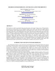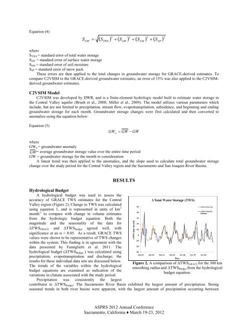Hydrological Budget A hydrological budget was used to assess the accuracy of GRACE TWS estimates for the Central Valley region (Figure 2). Change in TWS was calculated using equation 1, and is represented in units of km 3 month -1 to compare with change in volume estimates from the hydrologic budget equation. Both the magnitude and the seasonality of the data for TWS GRACE and TWS Budget agreed well, with significance at an = 0.05. As a result, GRACE TWS values were shown to be representative of TWS changes within the system. This finding is in agreement with the data presented by Famiglietti et al. 2011. The hydrological budget (ΔTWS Budget ) was calculated using precipitation, evapotranspiration and discharge; the results for these individual data sets are discussed below. The trends of the variables within the hydrological budget equations are examined as indication of the variations in climate associated with the study period. Precipitation was consistently the largest RESULTS Figure 2. A comparison of ΔTWS GRACE for the 300 km smoothing radius and ΔTWS Budget from the hydrological budget equation. contributor to ΔTWS Budget . The Sacramento River Basin exhibited the largest amount of precipitation. Strong seasonal trends in both river basins were apparent, with the largest amount of precipitation occurring between ASPRS 2012 Annual Conference Sacramento, California ♦ March 19-23, 2012
December and April during the region’s winter storm period with a range of 14.54 km 3 –25.83 km 3 . These results reflect the drought period from 2007–2009 following the above average precipitation year of 2006. The Sacramento River Basin experienced the largest loss in total evapotranspiration followed by the San Joaquin River Basin. As would be expected, evapotranspiration exhibited seasonal trends with the largest evapotranspiration values occurring in late spring to early summer (May, June, and July), and the lowest values during the winter months (December and January). The Sacramento River Basin, in comparison with the San Joaquin River Basin, consistently produced greater discharge. Discharge also exhibited seasonal trends that peaked between February and April (in occurrence with snow melt from the Sierras) before steadily declining through the months of June and December. The range of discharge varied from 1.63–6.89 km 3 in both the Sacramento and San Joaquin rivers. Storage Anomalies GRACE TWS anomalies exhibited similar trends for the Sacramento River Basin, the San Joaquin River Basin, and the Central Valley region. Storage anomalies increased after the winter rains and rapidly decreased throughout the drier summer months (Figure 3A). The Central Valley region produced the largest standard deviations about the mean (0.72 km 3 ± 19.05) followed by the San Joaquin (0.35 km 3 ± 9.86) and Sacramento (0.37 km 3 ± 9.55), respectively. Surface water storage anomalies demonstrated similar seasonal trends (Figure 3B). In general, surface water storage anomalies increased between 2002 and 2006, before decreasing at the onset of the drought period beginning in 2007. Soil moisture storage anomalies also exhibited seasonal trends that increased during the winter months and decreased during the drier summer months (Figure 3B). In general, the Sacramento and San Joaquin River Basins and the Central Valley displayed similar values (both in magnitude and seasonality) throughout the Figure 3. Hydrologic variable anomalies. (A) TWS anomalies from GRACE, (B) surface water storage anomalies from CDEC, (C) soil moisture storage anomalies from AMSR-E, and (D) snow pack anomalies from NOAA. length of the study. Snowpack storage anomalies exhibited pronounced winter and summer variations (Figure 3C). The winters between 2004 and 2006 produced the largest snowpack totals during the study period. Interestingly, the Sacramento and San Joaquin River Basins exhibited conflicting anomaly trends with anomaly values increasing for the Sacramento River Basin through the duration of the study period (with the exception of the winter in 2006– 2007) (Figure 3D). However, in the San Joaquin River Basin, snowpack anomalies increased until the winter of 2005–2006 before exhibiting a sharp and notable decrease for the rest of the study period. The Central Valley and the San Joaquin River Basin exhibit the largest seasonal fluctuations and differ significantly from the Sacramento ASPRS 2012 Annual Conference Sacramento, California ♦ March 19-23, 2012
Page 1 and 2: COMPARISON OF CHANGES IN GROUNDWATE
Page 3 and 4: Valley aquifer (52,000 km 2 ), it w
Page 5: Discharge. Real time daily mean dis
Page 9 and 10: Both GRACE and C2VSIM produced comp
Page 11 and 12: REFERENCES Brush, C.F., E.C. Dogrul

comparison of changes in groundwater storage using grace ... - asprs

You also want an ePaper? Increase the reach of your titles

Delete template?

Save as template?