Spectral Estimation Using a MUSIC Algorithm - Altera

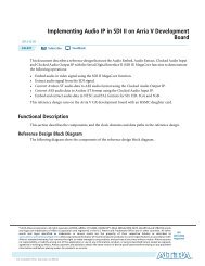
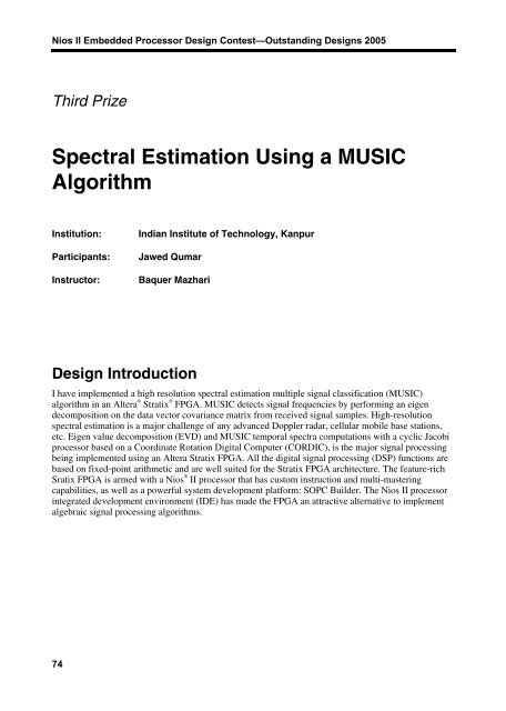
Nios II Embedded Processor Design Contest—Outstanding Designs 2005
Third Prize
Spectral Estimation Using a MUSIC
Algorithm
Institution:
Participants:
Instructor:
Indian Institute of Technology, Kanpur
Jawed Qumar
Baquer Mazhari
Design Introduction
I have implemented a high resolution spectral estimation multiple signal classification (MUSIC)
algorithm in an Altera ® Stratix ® FPGA. MUSIC detects signal frequencies by performing an eigen
decomposition on the data vector covariance matrix from received signal samples. High-resolution
spectral estimation is a major challenge of any advanced Doppler radar, cellular mobile base stations,
etc. Eigen value decomposition (EVD) and MUSIC temporal spectra computations with a cyclic Jacobi
processor based on a Coordinate Rotation Digital Computer (CORDIC), is the major signal processing
being implemented using an Altera Stratix FPGA. All the digital signal processing (DSP) functions are
based on fixed-point arithmetic and are well suited for the Stratix FPGA architecture. The feature-rich
Sratix FPGA is armed with a Nios ® II processor that has custom instruction and multi-mastering
capabilities, as well as a powerful system development platform: SOPC Builder. The Nios II processor
integrated development environment (IDE) has made the FPGA an attractive alternative to implement
algebraic signal processing algorithms.
74

Spectral Estimation Using a MUSIC Algorithm
Function Description
The MUSIC algorithm is a kind of directional of arrival (DOA) estimation technique based on eigen
value decomposition, which is also called the subspace-based method. Here, we consider a unitary
MUSIC algorithm. With this, the eigen decomposition of correlation (covariance) matrix in the MUSIC
algorithm can be solved with real numbers only. This system achieves high performance in EVD and
MUSIC angular spectra computation with a cyclic Jacobi processor on a CORDIC and spatial DFT
respectively. The unitary MUSIC computational flow involves the following steps:
1. Estimation of the correlation matrix, including unitary transform.
2. EVD of the correlation matrix.
3. Computation of the MUSIC spectrum.
4. Local Maximum detection.
I have implemented EVD via a CORDIC-based Jacobi processor. The EVD computation processor for
MUSIC DOA uses a CORDIC-based Jacobi method. The cyclic Jacobi processor computes real
symmetric eigenvalue problems by applying a sequence of orthonormal rotations to the left and right
sides of the target matrix (unitary transformed K X K real symmetric correlation matrix Ryy) as:
Where Wpq is an orthonormal plane rotation over an angle θ in the (p, q) plane whose elements are
Wpp = cos θ, Wpq = sinθ, Wqp = −sin θ, Wqq = cosθ (p > q). J is the multiple rotation of Wpq’s in
the cyclic-by-row manner of (p, q), which is called a Jacobi sweep, and the superscript T and subscript
K denote transposition and array length, respectively. This processor employed the hardware friendly
CORDIC algorithm for vector rotators and arctangent computers to solve the above equations, which
were the basic processing unit. Because the fixed-point operation is applied, of course approximation
errors exist. But when it was implemented with the above 16-bit precision, we could get reasonable
performance. In the next section, implementation angular spectrum is computed after the EVD step. See
Figure 1.
75

Nios II Embedded Processor Design Contest—Outstanding Designs 2005
Figure 1. System Overview
Re[ X
1
• X1
H ]
Re[ X
2
• X
2
H ]
...
...
Re[ X • X
H
M
]
M
...
Performance Parameters
The estimated performance of the dominant core functions is the number of occupied logic blocks in the
FPGA and f MAX
is the maximum clock frequency at which normal operation can be guaranteed. The
minimum computation time, tmin, is calculated by required clks * f MAX
. I assumed that less than 2
coherent/incoherent waves arrived at only 4-element uniform linear array antenna. For spectrum
generation, 256-point radix-4 complex fast Fourier transform (FFT) was employed and the FFT with
256 spatial data composed of N elements of the noise eigenvector and (256−N) zeroes interpolates the
spectrum fine and smoothly. All computations were performed by fixed-point arithmetic with 12-bit
input data from ADCs. On the other hand, the estimation accuracy of the EVD system depends on so
many factors that the proper assessment has some difficulties in detailed analysis. For example, the
effect of finite bit-length and bit-truncation by scaling in the fixed-point operation, the estimation errors
caused by non-uniform discrete wavefront, and so forth.
Design Architecture
The EVD of the input matrix X can be performed, as illustrated in Figure 2, using the well known
systolic array architecture. The rows of matrix X are fed as inputs to the array from the top, along with
the corresponding element of the vector y. The R and u values, held in each of the cells once all the
inputs have been passed through the matrix, are the outputs from the EVD. These values are
subsequently used to derive the coefficients using a back substitution technique.
76

Spectral Estimation Using a MUSIC Algorithm
Figure 2. EVD of the Input Matrix
The CORDIC rotation-based algorithm is implemented in a very efficient pipelined manner using a
triangular systolic array. The schematic is shown in Figure 3, for M = 4 antenna elements.
Figure 3. CORDIC Rotation-Based Algorithm Schematic
x 1 (t) x 2 (t - 1)
x 3 (t - 2)
y(t - 3)
A B D
Vec.
Rot.
Rot.
Rot.
F
( in )
in
0 1
Rot. Vec. Rot. Rot.
x i y i
n n
CPE
x out y out
0
Rot. Vec. Rot.
C
( out )
0
out
Rot
G
D
E
H
σΦ ,in
Re(x in ) Im(x in )
σΦ ,in
Φ - CPE
(|x in |)
Re(r)
Im(r)
Θ - CPE 1 Θ - CPE 2
σΦ ,out
σΦ ,out
e(t - 7)
Re(x out ) Im(x out )
(a)
(b)
The cells in the triangular array (A-B-C) store the elements of the evolving triangular matrix R[i], and
the ones in the right hand column (D-E) store the elements of the updated vector u[i]. The data flow is
from top to bottom, while the rotation angles are propagated from left to the right of the array. In this
implementation, the array entirely consists of CORDIC processor elements (CPEs), which work
completely synchronously, driven by a single global master clock. Because all the CPEs need the same
amount of time to perform their computations they never get flooded with data. Thereby, the CPEs
designated with Vec are configured to the “vectoring” mode of operation, and those labeled with Rot
operate in the “rotation” mode. Each row performs a given rotation, whereby the rotation angle is
determined by the CPE in vectoring mode at the beginning of the row. The rotation angle is passed to
the rotation CPEs to the right with one clock cycle delay, thus requiring the elements of the data vector
to be applied to the array in a time-staggered fashion, as indicated by the indices in Figure 3. To handle
the complex data, complex CORDIC is used. As shown above, it is comprised of three CPEs
interconnected according to figure 4b. In vectoring mode (Im(r m,m
) = 0), the imaginary part of the
complex value x m
is annihilated by the Φ-CPE and subsequently | x m
| is zeroed in θ-CPE 1
. The complex
Givens rotation is then coded by the two sequences of rotation coefficients {σ Φ,j } and {σ θ,j }. By applying
these rotation coefficients to a supercell configured to operate in the rotation mode, the incoming vector
(Re(x in
) Im(y in
)) T is rotated by Φ m
in the Φ-CPE and subsequently the real and imaginary parts of r m,n
and
x m,n
are each rotated by θ m
in θ-CPE 1
and θ-CPE 2
, respectively.
77

Nios II Embedded Processor Design Contest—Outstanding Designs 2005
The heart of the design is the EVD decomposer block. The hardware implementation is carried out
directly using systolic array. I worked this out first with a kind of direct mapping, where as many
CORDIC blocks are required. The aim was first to get the R matrix and U matrix from the given input
of X and Y matrix. The rest of the task is taken care of by the Nios II processor. The number of logic
elements used was very high. Also, the EVD update can be done very fast: this is not required for so
many practical applications, for example, a radar system where the interference environment changes in
milliseconds or hundreds of microseconds. So excess hardware utilization and achieving high speed is
of little interest. To address this problem, the array can be mapped to a reduced number of CPEs on a
time-shared basis.
Complex CORDIC blocks are required, so as to implement the complex data. Each complex CORDIC
block consists of three basic CORDIC blocks. I have implemented systolic array for four antenna
elements. As mentioned, this approach gave satisfactory output, but the problem with the scheme is that
it consumes too many logic elements, which is not practical. So, I have worked out another scheme
which does the same thing with only two complex CORDIC blocks. This approach is called mixed
mapping which consumes less logic elements. The benefit is achieved with the scheme, but latency also
will be there. This latency is unavoidable. The scheme is practical, as resource utilization is well within
the limits of the Stratix FPGA. This requires an additional state machine to control the operation. Out of
the two CORDIC blocks, one is for vectoring mode and another for rotating mode of operation.
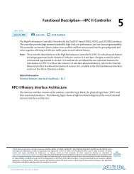
Figure 4 is the block diagram representation of the design.
Figure 4. Block Diagram
Avalon Bus
Input
Bank1
Input
Bank2
Multiplexer
Input
Buffer
EVD
Odd Bank
Even Bank
Nios II
Processor
The data on which EVD is to be carried out is in bank1 and bank2. The multiplexer will select the bank
alternately and will pass it to the input buffer. This input buffer is controlled, so when required, it is
being read and given to the EVD. The EVD will write data alternately in the odd and even memory
bank. This is because when Nios II is reading from one bank, the EVD will write data in the other
memory bank. The Nios II processor communicates with the peripheral using the Avalon ® bus.
Figure 5 is a schematic representation of the EVD. The input data is 32 bit and of complex nature. The
EVD requires two types of operations, namely boundary-cell and internal-cell operation. As we have
used a mixed mapping approach, the scheduling of the complex CORDIC block is a must here. This is
achieved at the cost of speed. The load enable signal initiates the EVD decomposition task. A separate
controller generates the load enable signal when required. The output of the EVD is intentionally stored
once in the odd memory bank and once in the even memory bank because, for example, if the Nios II
processor is reading from the odd bank, the EVD can write into the even memory bank and vice versa.
78

Spectral Estimation Using a MUSIC Algorithm
Figure 5. EVD Schematic Representation
clk
32-Bit Odd Memory
reset
32-Bit Data
load-en
EVD
32-Bit Even Memory
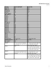
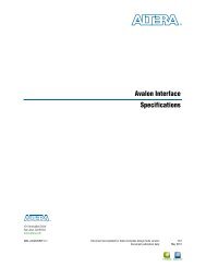
Figure 6 is a simplified view of the controller responsible for generating control signals, as necessary.
Figure 6. Controller
clk
reset
done_reset
cordic_clk
load_enable
Controller
data_sel_pass1
bank_sel
vec_rot_sel_pass1
rd_wr_x
vec_rot_sel_pass1
global_ress
done
cordic_clock_by2
read_address_out[5:0]
The register transfer level (RTL) view of the controller is shown in Figure 7.
It is a finite state machine that uses a counter and mealy state machine. It generates the following
control signals for different blocks. It is the central unit for the EVD processor. When the load_en signal
comes, as long as high loading of the data takes place, as soon as load_en goes low, the controller acts.
It generates:
1. bank select signal for switching the y memory bank data and address.
2. vec_rot_sel signal, which is used to multiplex between the vector and rotation modes of the
complex CORDIC.
3. address signal for writing into the memory and reading from the memory.
4. Done signal, which goes high when the EVD operation is over.
79

Nios II Embedded Processor Design Contest—Outstanding Designs 2005
Figure 7. RTL View of Controller
[2:0]
[2:0]
read_address_out[5:0]
vec_rot_sel_pass1
clk_en
reset_gen_counter
vec_rot_sel_pass1
reset
vec_rot_sel_pass2
clk
bank_end
1 bank_end_rdwr_dis
clk_en
address[4:0]
reg_gen_enZ2
reset
clk
1 clk_en ro[0]
ri[0]
tc_9_reg1
un1_bank_end_tc_mod
bank_end_tc_mod
1
row_end_gen_9
reset row_end
clk
clk_en
address[3:0]
data_read_gen1_tc [3:0]
bank_end_tc_out
data_sel_pass1
tc_bank_en_gen
vec_rot_sel_pass2
row_end_gen
reset
clk row_end
1
clk_en
address[3:0]
[3:0]
read_address_gen1_msb
row_end_gen
1
reset
row_end
clk
clk_en
address[3:0]
read_address_gen1_lsb
[3:0]
bank_sel_cnt
reg_genZ3
reg_gen_enZ2
1
reset
clk
row_end
clk_en
address[3:0]
reset
clk
ri[0]
ro[0]
reg_genZ3
reset
clk
ro[0]
ri[0]
1
reset
clk
clk_en
ri[0]
ro[0]
bank_sel
bank_sel_tc_gen1
[3:0]
input_data_read_sel
bank_sel_gen1
neg_edge_bank_sel
row_end_10
reg_genZ3
reg_genZ3
timing_cnt
reg_genZ3
reset
reset
cordic_clock
load_en
reset
clk
ro[0]
ri[0]
load_en_reg_rdwr
global_reset_rdwr
start
reset
output_en
clk
address[3:0]
[3:0]
rd_wr_gen1
[3]
rd_wr_x_sig
reset
clk
ro[0]
ri[0]
reg_rdwr1
clk
ro[0]
ri[0]
reg_rdwr2
rd_wr_x
clk
reg_genZ3
reg_genZ3
reset
done_reset
1
done_counter
reset
clk
clk_en
tc
reset
clk
ro[0]
ri[0]
reg_done1
clk
ro[0]
ri[0]
reg_done2
done
address[7:0]
done_inst
global_reset_out
global_reset_out
timing_cnt
start
reset
output_en
clk
address[3:0]
cordic_clk_by2_1
[3:0]
[2]
cordic_clk_by2
cordic_clk_by2
Figure 8 shows the complex CORDIC block and the equivalent RTL is shown in Figure 9.
Figure 8. Complex CORDIC
clk
xout_real_th[21:0]
reset
start
output_en
r_x_real_in[21:0]
r_x_imag_in[21:0]
Complex CORDIC
xout_real_th_next[21:0]
xout_imag_th[21:0]
xin_real[21:0]
xout_imag_th_next[21:0]
xin_imag[21:0]
vec_rot_sel
80

Spectral Estimation Using a MUSIC Algorithm
Figure 9. RTL of Complex CORDIC
vec_rot
clk
reset
R_x_real_in[21:0]
[21:0]
reg_gen_enZ2
reset
clk
1 ro[0]
clk_en
1
reg_gen_enZ2
reset
clk
clk_en
ri[0]
ro[0]
reg_gen_enZ1
reset
clk
ro[17:0]
clk_en
[17:0]
ri[17:0]
[17:0]
1
[21:0]
[21:0]
[17:0]
start
[21:0]
clk_en x_out[21:0]
xout_real_th[21:0]
[21:0]
output_en
[21:0]
y_out[21:0]
vec_rot_sel
[21:0]
result[17:0]
dataa[21:0]
[17:0]
datab[21:0]
zin[17:0]
vec_rot_theta_real
ri[0]
vec_rot_sel_delay2
theta_real_store
reset
reg_gen_enZ2
reset
vec_rot_sel_reg1
clk
output_en
1
clk
clk_en
ri[0]
ro[0]
vec_rot
clk
reset
vec_rot
output_delay
[21:0]
xin_imag[21:0]
start
xin_real[21:0]
[21:0]
reg_gen_enZ2
reset
clk
1
clk_en
ro[0]
vec_rot_sel
ri[0]
[17:0]
1
[21:0]
reg_gen_enZ1
reset
[21:0]
clk
[17:0]
ro[17:0]
clk_en
[17:0]
ri[17:0]
clk
reset
start
[21:0]
clk_en x_out[21:0]
output_en
y_out[21:0]
vec_rot_sel
[21:0]
result[17:0]
dataa[21:0]
datab[21:0]
zin[17:0]
vec_rot_inst
mux_genZ3
sel
mux_out[21:0]
[21:0]
A[21:0]
[21:0]
B[21:0]
mux_vec
start
1 [21:0]
[21:0] clk_en x_out[21:0]
xout_imag_th[21:0]
[21:0]
output_en
y_out[21:0]
[21:0]
xout_imag_th_next[21:0]
vec_rot_sel
[21:0]
[21:0]
result[17:0]
dataa[21:0]
[17:0]
[21:0]
datab[21:0]
[17:0]
zin[17:0]
vec_rot_theta_imag
vec_rot_sel_delay1
phi_store
reg_gen_enZ1
R_x_imag_in[21:0]
[21:0]
[17:0]
reset
clk
clk_en
ri[17:0]
ro[17:0]
[17:0]
theta_imag_store
This complex CORDIC block is the key block for EVD. It comprises three CORDIC blocks and one
phi-CORDIC block. These blocks are used for compensating the imaginary part of the complex input,
the two theta-CORDIC ones are for the real part and the other is for the imaginary part. Because we are
using a complex CORDIC in a time division multiplex manner, the angles phi and theta are stored in
vector mode and these angles are used subsequently in rotation mode. The output block is important, as
shown in Figure 10, for storing the final result and generating the control-signal-like interrupt when
EVD is over. It also provides all necessary addresses and bus control signals for interfacing with the
Nios II processor.
Figure 10. Output Block
load_en
reset
done
clk
cordic_clock
1
address_wr_op
reset
tc
clk
address[5:0]
clk_en
[5:0]
1
reg_gen_enZ4
reset
clk
ro[0]
clk_en
ri[0]
tc_reg_1
address_wr_op
reset
[5:0]
tc
clk
[5:0]
address[5:0]
1
clk_en
address_wirte_inst
[5:0]
mux_rd_wr_address_inst
sel
mux_genZ2
[5:0]
A[5:0]
[5:0]
mux_out[5:0]
B[5:0]
address_rd_wr[5:0]
address_read_inst
[5:0]
rd_wr
address_rd[5:0]
81

Nios II Embedded Processor Design Contest—Outstanding Designs 2005
CORDIC Architecture
I have implemented CORDIC as an iterative architecture that is a direct translation from CORDIC
equations.
The CORDIC rotator is normally operated in one of two modes. The first mode, called rotation mode,
rotates the input vector specified angle. The second mode, called vectoring, rotates the input vector to
the x-axis while recording the angle required to make that rotation.
Rotation Mode
In rotation mode, the angle accumulator is initialized with the desired rotation angle. The rotation
decision at each iteration is made to diminish the magnitude of the residual angle accumulator. The
decision at each iteration is therefore based on the sign of the residual angle after each step.
Vectoring Mode
In vectoring mode, the CORDIC rotator rotates the input vector through whatever angle is necessary to
align the result vector with the x axis. The result of the vectoring operation is a rotation angle and the
scaled magnitude of the original vector (x component of the result). The vectoring function works by
seeking to minimize the y component of the residual vector at each rotation. The sign of the residual y
component is used to determine which direction to rotate next.
An iterative CORDIC architecture can be obtained by duplicating each of the three difference equations
in hardware as shown in Figure 11. The decision function, d i
, is driven by the sign of the y or z register,
depending on whether it is operating in the rotation or vectoring mode. In operation, the initial values
are loaded via multiplexers into the x, y and z registers. Then on each of the next n clock cycles, the
values from the registers are passed through the shifters and adder-subtractors and the result is placed
back in the registers. At each iteration, the shifters are modified to cause the desired shift for the
operation. Likewise, at each iteration, the ROM address is incremented so that the appropriate
elementary angle value is presented to the z adder-subtractor. On the last iteration, the results are read
directly from the adder-subtractors.
82

Spectral Estimation Using a MUSIC Algorithm
Figure 11. Equations in Hardware
Iterative Cordic Sructure
mux
reg
+/-
>>n
£mdi
>>n
Sign(y i )
+/-
reg
mux
y 0
ROM
Sign(z i )
+/-
reg
-di
mux
z 0
x 0
d i
x
y
z
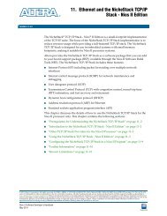
Figure 12 shows a hardware-level simulation result. Hardware-level simulations were performed by the
direct measurements with only the DSP part of real hardware, to efficiently evaluate the validity of the
system. I used the input data made by an offline PC in advance, and obtained the results with real
hardware operation. With these hardware-level simulations, we could verify the function of the digital
signal processor. In this simulation, it was assumed that 2 coherent (or fully correlated) waves were
impinging at 4 antennas from the DOAs of -15 and 20 degrees, respectively. And two waves were the
same power and the input SNR was 15 dB. For the spectrum computation, the FFT of 256 points,
including 3-spatial data of the noise eigenvector’s elements (1 dimension was used for spatial
smoothing) and 253 zeroes, was applied. The final result waveform output is shown in Figure 13, which
shows CORDIC and EVD decomposed values.
83

Nios II Embedded Processor Design Contest—Outstanding Designs 2005
Figure 12: Hardware Simulation Result of MUSIC (EVD) & Its Inverse (SNR 15 dB)
(4 Antenna with 2 Coherent Waves at -15 & 20 Degrees)
Magnitude (dB)
0
-5
-10
-15
-20
-25
-30
-35
-40
-45
Local Minimum
8
7
6
5
4
3
2
1
-50 -100 -80 -60 -40 -20 0 20 40 60 80
0 100
x10 4
10
9
Magnitude
Angle (Degree)
Figure 13. Final Result Waveform
FPGA Implementation
As discussed earlier, I am going to develop the EVD, which is the IP for the system. It is the
responsibility of the Nios II processor to read the values of the R and U matrix from the EVD. The
Nios II processor is responsible for the two tasks namely: 1) reading the R and U matrix 2) back
substitution. Back substitution involves calculating the weights and putting them back.
I developed the software for the above mentioned tasks. It takes approximately 57 µs to accomplish the
specified task (4 antenna elements). This information is useful to calculate the throughput of the system.
The software part also includes the interrupt service routine such that the Nios II processor will read the
data and do the back substitution repetitively. The duration between each interrupt is also programmable
and in synchronization with the system clock. For the above tasks I developed two peripherals, with one
master and one slave each. The master reads data from memory and the Nios II processor does the
necessary calculation for generating the new weights. The slave interface, which consists of a counter, is
generating interrupt. The processor acknowledges the interrupt after 8 µs so that is to be taken care of
while periodically generating the interrupt.
84

Spectral Estimation Using a MUSIC Algorithm
The hardware-software co-simulation in the ModelSim ® tool helped me to resolve the problem, and to
estimate the time taken by the processor to acknowledge the interrupt. The program developed for the
back substitution is not fixed for four antenna elements, but it is a general program, applicable to any
number of antenna elements.
The Avalon bus is a simple bus architecture designed for connecting on-chip processors and peripherals
together into a system-on-a-programmable-chip (SOPC) solution. See Figure 14. It is an interface that
specifies the port connections between master and slave components. Basic Avalon bus transactions
transfer a single byte, half word, or word between a master and slave peripheral. After the completion of
a transfer, the bus is available on the next clock cycle for any another transaction.
Figure 14. Avalon Bus
Avalon Bus
Nios II
Processor C_r C_i
Data &
Program
Memory
R_r R_i U_r U_i
Mixed Mode EVD_Decomposer
Some key features of the Avalon bus are:
■
■
■
■
■
■
Memory and peripherals may be mapped anywhere within the 32- bit address space.
All Avalon signals are synchronized to the Avalon bus clock, which simplifies the timing behavior
of the Avalon bus and facilitates integration with high-speed peripherals.
Separate, dedicated address and data paths provide the easy interface to on chip user logic.
Peripherals do not need to decode data and address bus cycles.
The Avalon bus automatically generates chip select signals for all peripherals, greatly simplifying
the design of Avalon peripherals.
Multiple master peripherals can reside on the Avalon bus. The Avalon bus generates the required
arbitration logic.
The Avalon bus also handles the details of transferring data between peripherals with mismatched
data widths.
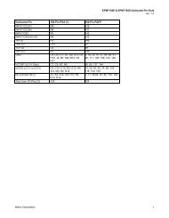
Device Utilization Summary
Family
Stratix
Device
EP1S10F780C6ES
Total logic elements 8,236 / 10,570 ( 77 % )
Total pins 34 / 427 ( 31 % )
Total memory bits 61,856 / 920,448 ( 6 % )
DSP block 9-bit elements 8 / 48 ( 16 % )
Total phase-locked loops (PLLs) 1 / 6 ( 16 % )
Total DLLs 0 / 2 ( 0 % )
85

Nios II Embedded Processor Design Contest—Outstanding Designs 2005
Test Results & Comparison
I have undergone a full design cycle of an SOPC implementation, i.e., hardware-software co-design,
integration of peripherals with Avalon bus, etc. A hardware-based approach is accelerating the
performance. The new hardware-based computing will solve the bottleneck of algorithmic signal
processing. It is discovered that, if a CORDIC block is implemented in software only, it takes 8,600
clock cycles to complete the vectoring mode of operation as opposed to what I have achieved: 16 clock
cycles to accomplish the same task in hardware. This result can motivate a CORDIC-based EVD. With
respect to accuracy, if we compare the Arctan function implementation in software only, it requires
approximately 20,000 clock cycles to achieve the same accuracy as the Arctan IP developed with a
hardware approach. We achieved the desired functionality with the Nios II processor running at a clock
speed of 50 MHz on a Stratix board. Our design of the EVD IP only takes 55 percent of the chip area on
the Stratix FPGA.
Performance Comparison
Software Approach
Method CORDIC (Cycles) CORDIC EVD (Cycles)
Direct Equation 8,600 (172 us) 90,3000 (18 us)
Arctan Series Expansion 20,000 (400 us) 2,100,000 (42 ms)
Hardware Approach
CORDIC (Cycles)
CORDIC EVD (Cycles)
16
16 (EVD update latency will
be 16 cycles) = 320 ns
Logic Elements Utilization for EVD Decomposer
Method
Logic Elements
Direct Mapping 34,055
Mapping Each Row 7,811
Mixed Mapping 4,946
Design Features
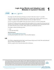
I tried different mapping architectures for optimum implementation. This section shows different
mapping for seven antenna elements. Figure 15 shows direct mapping.
86

Spectral Estimation Using a MUSIC Algorithm
Figure 15. Direct Mapping
Figure 16 shows mix mapping and Figure 17 shows row mapping. Round blocks indicate the vectoring
mode of operation. Square blocks indicate the rotating mode of operation.
Figure 16. Mix Mapping
87

Nios II Embedded Processor Design Contest—Outstanding Designs 2005
Figure 17. Row Mapping
Conclusion
From the above design, it is evident that for real-time implementation of computationally intensive
algebraic signal processing algorithms, an FPGA-based SOPC solution is a promising, futuristic
technology.
88

Altera, The Programmable Solutions Company, the stylized Altera logo, specific device designations, and all other
words and logos that are identified as trademarks and/or service marks are, unless noted otherwise, the trademarks
and service marks of Altera Corporation in the U.S. and other countries. All other product or service names are the
property of their respective holders. Altera products are protected under numerous U.S. and foreign patents and
pending applications, mask work rights, and copyrights.