Photon-Induced Near Field Electron Microscopy - California Institute ...

|E| 2
Re[E x ] Im[F 0 ]
|F 0 | 2
x-polarized
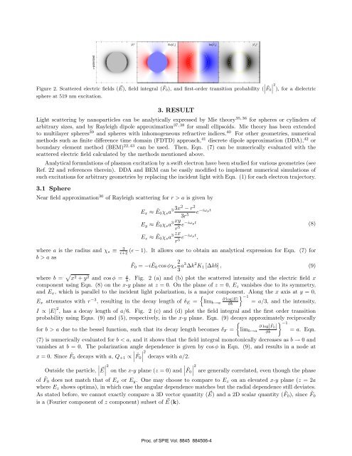
Figure 2. Scattered electric fields ( E), ⃗ field integral ( ˜F 0), and first-order transition probability ( ˛ ˜F 0˛˛˛2
), for a dielectric
sphere at 519 nm excitation.
3. RESULT
Light scattering by nanoparticles can be analytically expressed by Mie theory 35, 36 for spheres or cylinders of
arbitrary sizes, and by Rayleigh dipole approximation 37, 38 for small ellipsoids. Mie theory has been extended
to multilayer spheres 39 and spheres with inhomogeneous refractive indices. 40 For other geometries, numerical
methods such as finite difference time domain (FDTD) approach, 41 discrete dipole approximation (DDA), 42 or
boundary element method (BEM) 22, 43 can be used. Then, Eqn. (7) can be numerically evaluated with the
scattered electric field calculated by the methods mentioned above.
Analytical formulations of plasmon excitation by a swift electron have been studied for various geometries (see
Ref. 22 and references therein). DDA and BEM can be easily modified to implement numerical simulations of
such excitations for arbitrary geometries by replacing the incident light with Eqn. (1) for each electron trajectory.
3.1 Sphere
Near field approximation 30 of Rayleigh scattering for r > a is given by
where a is the radius and χ s ≡ 3
b > a as
ɛ+2
E x ≈ Ẽ0χ s a 3 3x2 − r 2
3r 5
E y ≈ Ẽ0χ s a 3 xy
r 5 e−iωpt
E z ≈ Ẽ0χ s a 3 zx
r 5 e−iωpt ,
e −iωpt
(ɛ − 1). It allows one to obtain an analytical expression for Eqn. (7) for
˜F 0 = −iẼ0 cos φχ s
2
3 a3 ∆k 2 K 1 [∆kb] , (9)
where b = √ x 2 + y 2 and cos φ = x b
. Fig. 2 (a) and (b) plot the scattered intensity and the electric field x
component using Eqn. (8) on the x-y plane at z = 0. On the plane of z = 0, E z vanishes due to its symmetry,
and E x , which is parallel to the incident light polarization, is a major component. Along the x axis at y = 0,
{
E x attenuates with r −3 , resulting in the decay length of δ E =
lim b→a
∂ log|E|
∂b
(8)
} −1
= a/3, and the intensity,
I ∝ |E| 2 , has a decay length of a/6. Fig. 2 (c) and (d) plot the field integral and the first order transition
probability using Eqns. (9) and (5), respectively, in the x-y plane. Eqn. (9) decays approximately reciprocally
{
} −1
∂ log|
for b > a due to the bessel function, such that its decay length becomes δ F = lim ˜F 0|
b→a ∂b
= a. Eqn.
(7) is numerically evaluated for b < a, and it shows that the field integral monotonically decreases as b → 0 and
vanishes at b = 0. The polarization angle dependence is given by cos φ in Eqn. (9), and results in a node at
x = 0. Since ˜F 0 decays with a, Q +1 ∝ ∣ ˜F
∣ ∣∣
2
0 decays with a/2.
Outside the particle, ∣E
⃗ ∣ 2 on the x-y plane (z = 0) and ∣ ˜F
∣ ∣∣
2
0 are generally correlated, even though the phase
of ˜F 0 does not match that of E x or E y . One may choose to compare to E z on an elevated x-y plane (z = 2a
where E z shows optima), in which case the angular dependence matches but the radial dependence still deviates.
As stated before, we cannot exactly compare a 3D vector quantity ( ⃗ E) and a 2D scalar quantity ( ˜F 0 ), since ˜F 0
is a (Fourier component of z component) subset of ⃗ E (k).
Proc. of SPIE Vol. 8845 884506-4