Waveguides - ieeetsu
Waveguides - ieeetsu
Waveguides - ieeetsu

Create successful ePaper yourself
Turn your PDF publications into a flip-book with our unique Google optimized e-Paper software.
www.ece.rutgers.edu/∼orfanidi/ewa 261<br />
262 Electromagnetic Waves & Antennas – S. J. Orfanidis – June 21, 2004<br />
∫<br />
P T = P z dS ,<br />
S<br />
where P z = 1 2 Re(E × H∗ )·ẑ (8.2.1)<br />
It is easily verified that only the transverse components of the fields contribute to<br />
the power flow, that is, P z can be written in the form:<br />
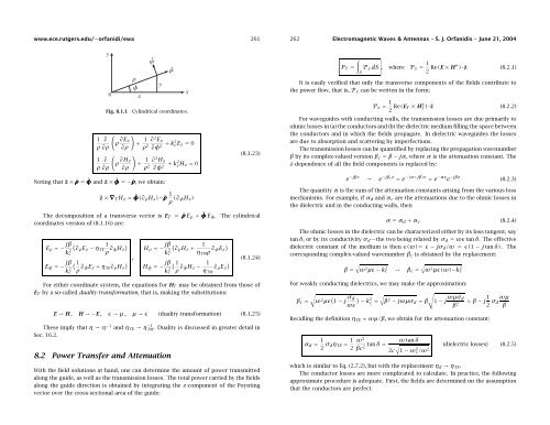
Fig. 8.1.1<br />
Cylindrical coordinates.<br />
(<br />
1 ∂<br />
ρ ∂E )<br />
z<br />
+ 1 ∂ 2 E z<br />
ρ ∂ρ ∂ρ ρ 2 ∂φ + 2 k2 cE z = 0<br />
(<br />
1 ∂<br />
ρ ∂H )<br />
z<br />
+ 1 ∂ 2 H z<br />
ρ ∂ρ ∂ρ ρ 2 ∂φ + 2 k2 c H z = 0<br />
(8.1.23)<br />
P z = 1 2 Re(E T × H ∗ T )·ẑ (8.2.2)<br />
For waveguides with conducting walls, the transmission losses are due primarily to<br />
ohmic losses in (a) the conductors and (b) the dielectric medium filling the space between<br />
the conductors and in which the fields propagate. In dielectric waveguides the losses<br />
are due to absorption and scattering by imperfections.<br />
The transmission losses can be quantified by replacing the propagation wavenumber<br />
β by its complex-valued version β c = β − jα, where α is the attenuation constant. The<br />
z-dependence of all the field components is replaced by:<br />
Noting that ẑ × ˆρ = ˆφ and ẑ × ˆφ =−ˆρ, we obtain:<br />
ẑ ×∇ T H z = ˆφ(∂ ρ H z )−ˆρ 1 ρ (∂ φH z )<br />
The decomposition of a transverse vector is E T = ˆρE ρ + ˆφE φ . The cylindrical<br />
coordinates version of (8.1.16) are:<br />
E ρ =− jβ ( 1<br />
∂ρ<br />
k 2 E z − η TE<br />
c<br />
ρ ∂ )<br />
φH z<br />
E φ =− jβ ( 1<br />
k 2 c ρ ∂ ) ,<br />
φE z + η TE ∂ ρ H z<br />
H ρ =− jβ (<br />
∂ρ<br />
kc<br />
2 H z + 1<br />
η TM ρ ∂ )<br />
φE z<br />
H φ =− jβ ( 1<br />
kc<br />
2 ρ ∂ φH z − 1 )<br />
∂ ρ E z<br />
η TM<br />
(8.1.24)<br />
For either coordinate system, the equations for H T may be obtained from those of<br />
E T by a so-called duality transformation, that is, making the substitutions:<br />
E → H , H →−E , ɛ → µ, µ→ ɛ (duality transformation) (8.1.25)<br />
These imply that η → η −1 and η TE → η −1<br />
TM. Duality is discussed in greater detail in<br />
Sec. 16.2.<br />
8.2 Power Transfer and Attenuation<br />
With the field solutions at hand, one can determine the amount of power transmitted<br />
along the guide, as well as the transmission losses. The total power carried by the fields<br />
along the guide direction is obtained by integrating the z-component of the Poynting<br />
vector over the cross-sectional area of the guide:<br />
e −jβz → e −jβcz = e −(α+jβ)z = e −αz e −jβz (8.2.3)<br />
The quantity α is the sum of the attenuation constants arising from the various loss<br />
mechanisms. For example, if α d and α c are the attenuations due to the ohmic losses in<br />
the dielectric and in the conducting walls, then<br />
α = α d + α c (8.2.4)<br />
The ohmic losses in the dielectric can be characterized either by its loss tangent, say<br />
tan δ, or by its conductivity σ d —the two being related by σ d = ωɛ tan δ. The effective<br />
dielectric constant of the medium is then ɛ(ω)= ɛ − jσ d /ω = ɛ(1 − j tan δ). The<br />
corresponding complex-valued wavenumber β c is obtained by the replacement:<br />
β =<br />
√<br />
ω 2 µɛ − k 2 c → β c =<br />
√<br />
ω 2 µɛ(ω)−k 2 c<br />
For weakly conducting dielectrics, we may make the approximation:<br />
√<br />
β c =<br />
ω 2 µɛ ( 1 − j σ d<br />
ωɛ<br />
) √<br />
√<br />
− k<br />
2<br />
c = β 2 − jωµσ d = β 1 − j ωµσ d<br />
≃ β − j 1 β 2<br />
2 σ ωµ<br />
d<br />
β<br />
Recalling the definition η TE = ωµ/β, we obtain for the attenuation constant:<br />
α d = 1 2 σ dη TE = 1 2<br />
ω 2<br />
βc 2 tan δ =<br />
ω tan δ<br />
√1<br />
(dielectric losses) (8.2.5)<br />
2c − ω 2 c/ω 2<br />
which is similar to Eq. (2.7.2), but with the replacement η d → η TE .<br />
The conductor losses are more complicated to calculate. In practice, the following<br />
approximate procedure is adequate. First, the fields are determined on the assumption<br />
that the conductors are perfect.