Waveguides - ieeetsu

More documents

Recommendations

Info

www.ece.rutgers.edu/∼orfanidi/ewa 261 262 Electromagnetic Waves & Antennas – S. J. Orfanidis – June 21, 2004 ∫ P T = P z dS , S where P z = 1 2 Re(E × H∗ )·ẑ (8.2.1) It is easily verified that only the transverse components of the fields contribute to the power flow, that is, P z can be written in the form: Fig. 8.1.1 Cylindrical coordinates. ( 1 ∂ ρ ∂E ) z + 1 ∂ 2 E z ρ ∂ρ ∂ρ ρ 2 ∂φ + 2 k2 cE z = 0 ( 1 ∂ ρ ∂H ) z + 1 ∂ 2 H z ρ ∂ρ ∂ρ ρ 2 ∂φ + 2 k2 c H z = 0 (8.1.23) P z = 1 2 Re(E T × H ∗ T )·ẑ (8.2.2) For waveguides with conducting walls, the transmission losses are due primarily to ohmic losses in (a) the conductors and (b) the dielectric medium filling the space between the conductors and in which the fields propagate. In dielectric waveguides the losses are due to absorption and scattering by imperfections. The transmission losses can be quantified by replacing the propagation wavenumber β by its complex-valued version β c = β − jα, where α is the attenuation constant. The z-dependence of all the field components is replaced by: Noting that ẑ × ˆρ = ˆφ and ẑ × ˆφ =−ˆρ, we obtain: ẑ ×∇ T H z = ˆφ(∂ ρ H z )−ˆρ 1 ρ (∂ φH z ) The decomposition of a transverse vector is E T = ˆρE ρ + ˆφE φ . The cylindrical coordinates version of (8.1.16) are: E ρ =− jβ ( 1 ∂ρ k 2 E z − η TE c ρ ∂ ) φH z E φ =− jβ ( 1 k 2 c ρ ∂ ) , φE z + η TE ∂ ρ H z H ρ =− jβ ( ∂ρ kc 2 H z + 1 η TM ρ ∂ ) φE z H φ =− jβ ( 1 kc 2 ρ ∂ φH z − 1 ) ∂ ρ E z η TM (8.1.24) For either coordinate system, the equations for H T may be obtained from those of E T by a so-called duality transformation, that is, making the substitutions: E → H , H →−E , ɛ → µ, µ→ ɛ (duality transformation) (8.1.25) These imply that η → η −1 and η TE → η −1 TM. Duality is discussed in greater detail in Sec. 16.2. 8.2 Power Transfer and Attenuation With the field solutions at hand, one can determine the amount of power transmitted along the guide, as well as the transmission losses. The total power carried by the fields along the guide direction is obtained by integrating the z-component of the Poynting vector over the cross-sectional area of the guide: e −jβz → e −jβcz = e −(α+jβ)z = e −αz e −jβz (8.2.3) The quantity α is the sum of the attenuation constants arising from the various loss mechanisms. For example, if α d and α c are the attenuations due to the ohmic losses in the dielectric and in the conducting walls, then α = α d + α c (8.2.4) The ohmic losses in the dielectric can be characterized either by its loss tangent, say tan δ, or by its conductivity σ d —the two being related by σ d = ωɛ tan δ. The effective dielectric constant of the medium is then ɛ(ω)= ɛ − jσ d /ω = ɛ(1 − j tan δ). The corresponding complex-valued wavenumber β c is obtained by the replacement: β = √ ω 2 µɛ − k 2 c → β c = √ ω 2 µɛ(ω)−k 2 c For weakly conducting dielectrics, we may make the approximation: √ β c = ω 2 µɛ ( 1 − j σ d ωɛ ) √ √ − k 2 c = β 2 − jωµσ d = β 1 − j ωµσ d ≃ β − j 1 β 2 2 σ ωµ d β Recalling the definition η TE = ωµ/β, we obtain for the attenuation constant: α d = 1 2 σ dη TE = 1 2 ω 2 βc 2 tan δ = ω tan δ √1 (dielectric losses) (8.2.5) 2c − ω 2 c/ω 2 which is similar to Eq. (2.7.2), but with the replacement η d → η TE . The conductor losses are more complicated to calculate. In practice, the following approximate procedure is adequate. First, the fields are determined on the assumption that the conductors are perfect.
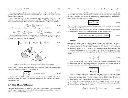
www.ece.rutgers.edu/∼orfanidi/ewa 263 264 Electromagnetic Waves & Antennas – S. J. Orfanidis – June 21, 2004 Second, the magnetic fields on the conductor surfaces are determined and the corresponding induced surface currents are calculated by J s = ˆn × H, where ˆn is the outward normal to the conductor. Third, the ohmic losses per unit conductor area are calculated by Eq. (2.8.7). Figure 8.2.1 shows such an infinitesimal conductor area dA = dl dz, where dl is along the cross-sectional periphery of the conductor. Applying Eq. (2.8.7) to this area, we have: dP loss dA = dP loss dldz = 1 2 R s|J s | 2 (8.2.6) where R s is the surface resistance of the conductor given by Eq. (2.8.4), √ √ √ ωµ ωɛ R s = 2σ = η 2σ = 1 2 δωµ , δ = 2 = skin depth (8.2.7) ωµσ Integrating Eq. (8.2.6) around the periphery of the conductor gives the power loss per unit z-length due to that conductor. Adding similar terms for all the other conductors gives the total power loss per unit z-length: P ′ loss = dP loss dz ∮ ∮ = 1 C a 2 R s|J s | 2 1 dl + C b 2 R s|J s | 2 dl (8.2.8) One common property of all three types of modes is that the transverse fields E T , H T are related to each other in the same way as in the case of uniform plane waves propagating in the z-direction, that is, they are perpendicular to each other, their cross-product points in the z-direction, and they satisfy: H T = 1 η T ẑ × E T (8.3.1) where η T is the transverse impedance of the particular mode type, that is, η, η TE ,η TM in the TEM, TE, and TM cases. Because of Eq. (8.3.1), the power flow per unit cross-sectional area described by the Poynting vector P z of Eq. (8.2.2) takes the simple form in all three cases: TEM modes P z = 1 2 Re(E T × H ∗ T )·ẑ = 1 2η T |E T | 2 = 1 2 η T|H T | 2 (8.3.2) In TEM modes, both E z and H z vanish, and the fields are fully transverse. One can set E z = H z = 0 in Maxwell equations (8.1.5), or equivalently in (8.1.16), or in (8.1.17). From any point view, one obtains the condition k 2 c = 0, or ω = βc. For example, if the right-hand sides of Eq. (8.1.17) vanish, the consistency of the system requires that η TE = η TM , which by virtue of Eq. (8.1.13) implies ω = βc. It also implies that η TE ,η TM must both be equal to the medium impedance η. Thus, the electric and magnetic fields satisfy: H T = 1 η ẑ × E T (8.3.3) Fig. 8.2.1 Conductor surface absorbs power from the propagating fields. These are the same as in the case of a uniform plane wave, except here the fields are not uniform and may have a non-trivial x, y dependence. The electric field E T is determined from the rest of Maxwell’s equations (8.1.5), which read: where C a and C b indicate the peripheries of the conductors. Finally, the corresponding attenuation coefficient is calculated from Eq. (2.6.22): α c = P′ loss (conductor losses) (8.2.9) 2P T Equations (8.2.1)–(8.2.9) provide a systematic methodology by which to calculate the transmitted power and attenuation losses in waveguides. We will apply it to several examples later on. 8.3 TEM, TE, and TM modes The general solution described by Eqs. (8.1.16) and (8.1.19) is a hybrid solution with nonzero E z and H z components. Here, we look at the specialized forms of these equations in the cases of TEM, TE, and TM modes. ∇ T × E T = 0 ∇ T · E T = 0 (8.3.4) These are recognized as the field equations of an equivalent two-dimensional electrostatic problem. Once this electrostatic solution is found, E T (x, y), the magnetic field is constructed from Eq. (8.3.3). The time-varying propagating fields will be given by Eq. (8.1.1), with ω = βc. (For backward moving fields, replace β by −β.) We explore this electrostatic point of view further in Sec. 9.1 and discuss the cases of the coaxial, two-wire, and strip lines. Because of the relationship between E T and H T , the Poynting vector P z of Eq. (8.2.2) will be: P z = 1 2 Re(E T × H ∗ T )·ẑ = 1 2η |E T| 2 = 1 2 η|H T| 2 (8.3.5)
Page 1 and 2: 256 Electromagnetic Waves & Antenna
Page 3: www.ece.rutgers.edu/∼orfanidi/ewa
Page 7 and 8: www.ece.rutgers.edu/∼orfanidi/ewa

Waveguides - ieeetsu

Create successful ePaper yourself

Delete template?

Save as template?