Tracer Interpretation Using Temporal Moments on a Spreadsheet G
Tracer Interpretation Using Temporal Moments on a Spreadsheet G
Tracer Interpretation Using Temporal Moments on a Spreadsheet G

You also want an ePaper? Increase the reach of your titles
YUMPU automatically turns print PDFs into web optimized ePapers that Google loves.
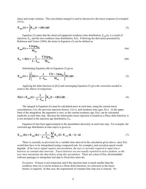
times and swept volumes. The c<strong>on</strong>voluti<strong>on</strong> integral is used to dec<strong>on</strong>volve the tracer resp<strong>on</strong>se (Levenspiel<br />
1972):<br />
t<br />
<br />
E (t) E (t )E(<br />
)<br />
d<br />
(3)<br />
app<br />
0<br />
in<br />
Equati<strong>on</strong> (3) states that the observed (apparent) residence time distributi<strong>on</strong>, E app (t), is a result of<br />
injecti<strong>on</strong>, E in, and the true residence time distributi<strong>on</strong>, E(t). Following the derivati<strong>on</strong> presented by<br />
Robins<strong>on</strong> and Tester (1984), the terms in Equati<strong>on</strong> (3) can be defined as<br />
E<br />
app<br />
C(t) qinj<br />
(t) (4a)<br />
M<br />
inj<br />
E<br />
in<br />
1 C(t) qinj<br />
(t)<br />
. (4b)<br />
1 f M<br />
loss<br />
inj<br />
Substituting Equati<strong>on</strong> (4b) in Equati<strong>on</strong> (3) gives<br />
t<br />
<br />
1 C(t )<br />
q<br />
<br />
inj<br />
E<br />
app(t)<br />
(t)<br />
<br />
E(<br />
)<br />
d<br />
. (5)<br />
1 f<br />
0 loss<br />
Minj<br />
<br />
Applying the delta functi<strong>on</strong> <strong>on</strong> [0,t] and rearranging Equati<strong>on</strong> (5) give the correcti<strong>on</strong> needed to<br />
remove the effects of reinjecti<strong>on</strong>:<br />
t<br />
1<br />
E (t) Eapp(t)<br />
Ein(t<br />
)E(<br />
)<br />
d<br />
. (6)<br />
1 f<br />
loss<br />
0<br />
The integral in Equati<strong>on</strong> (6) must be calculated anew at each time, using the current tracer<br />
c<strong>on</strong>centrati<strong>on</strong>, C(t), the previous injecti<strong>on</strong> history, C(t-), and residence time ages, E(). At the upper<br />
limit of the integrati<strong>on</strong>, the argument is zero, so the current residence age, E(t), can be calculated<br />
explicitly at each time step. Because the initial pulse tracer injecti<strong>on</strong> is treated as a Dirac delta functi<strong>on</strong>, it<br />
is not included in the injecti<strong>on</strong> age distributi<strong>on</strong>, E in .<br />
Equati<strong>on</strong> (6) has been approximated in the spreadsheet discretely at each time step. For example, the<br />
corrected age distributi<strong>on</strong> at time step k is given as<br />
E<br />
corr<br />
(k) E<br />
app<br />
1<br />
(k) <br />
1 f<br />
k 1<br />
<br />
loss i1<br />
E<br />
in<br />
(i) E<br />
corr<br />
(k i) t<br />
. (7)<br />
There is currently no provisi<strong>on</strong> for a variable time interval in the calculati<strong>on</strong> given above, since E(t)<br />
would then have to be interpolated (using a trapazoid rule, for example), and executi<strong>on</strong> speed would<br />
degrade. If the tracer signal requires dec<strong>on</strong>voluti<strong>on</strong>, the user is currently required to input tracer<br />
histories at c<strong>on</strong>stant time intervals. <str<strong>on</strong>g>Tracer</str<strong>on</strong>g> histories are not usually reported in such a fashi<strong>on</strong>, so the<br />
user must interpolate the data before using this spreadsheet. There are a host of free, downloadable<br />
software packages to interpolate real data to fixed time intervals.<br />
Excepti<strong>on</strong>: If tracer is not reinjected, and if the injecti<strong>on</strong> time is much smaller than the<br />
residence time (so it can be treated as a Dirac delta functi<strong>on</strong>), no correcti<strong>on</strong> to the tracer<br />
history is required. In that case, the requirement of c<strong>on</strong>stant time step size is relaxed. No<br />
4