Space Vector Modulated – Direct Torque Controlled (DTC – SVM ...
Space Vector Modulated – Direct Torque Controlled (DTC – SVM ...
Space Vector Modulated – Direct Torque Controlled (DTC – SVM ...

Create successful ePaper yourself
Turn your PDF publications into a flip-book with our unique Google optimized e-Paper software.
Warsaw University of Technology<br />
Faculty of Electrical Engineering<br />
Institute of Control and Industrial Electronics<br />
Ph.D. Thesis<br />
Marcin Żelechowski, M. Sc.<br />
<strong>Space</strong> <strong>Vector</strong> <strong>Modulated</strong> <strong>–</strong> <strong>Direct</strong><br />
<strong>Torque</strong> <strong>Controlled</strong> (<strong>DTC</strong> <strong>–</strong> <strong>SVM</strong>)<br />
Inverter <strong>–</strong> Fed Induction Motor Drive<br />
Thesis supervisor<br />
Prof. Dr Sc. Marian P. Kaźmierkowski<br />
Warsaw <strong>–</strong> Poland, 2005
Acknowledgements<br />
The work presented in the thesis was carried out during author’s Ph.D. studies at the<br />
Institute of Control and Industrial Electronics in Warsaw University of Technology,<br />
Faculty of Electrical Engineering. Some parts of the work were realized in cooperation<br />
with foreign Universities:<br />
• University of Nevada, Reno, USA (US National Science Foundation grant <strong>–</strong><br />
Prof. Andrzej Trzynadlowski),<br />
• University of Aalborg, Denmark (Prof. Frede Blaabjerg),<br />
and company:<br />
• Power Electronics Manufacture <strong>–</strong> „TWERD”, Toruń, Poland.<br />
First of all, I would like to express gratitude Prof. Marian P. Kaźmierkowski for the<br />
continuous support and help during work of the thesis. His precious advice and<br />
numerous discussions enhanced my knowledge and scientific inspiration.<br />
I am grateful to Prof. Andrzej Sikorski from the Białystok Technical University and<br />
Prof. Włodzimierz Koczara from the Warsaw University of Technology for their<br />
interest in this work and holding the post of referee.<br />
Specially, I am indebted to my friend Dr Paweł Grabowski for support and<br />
assistance.<br />
Furthermore, I thank my colleagues from the Intelligent Control Group in Power<br />
Electronics for their support and friendly atmosphere. Specially, to Dr Dariusz Sobczuk,<br />
Dr Mariusz Malinowski, Dr Mariusz Cichowlas, and Dariusz Świerczyńki M.Sc.<br />
Finally, I would like thank to my whole family, particularly my parents for their love<br />
and patience.
Contents<br />
1. Introduction 1<br />
Pages<br />
2. Voltage Source Inverter Fed Induction Motor Drive 6<br />
2.1. Introduction 6<br />
2.2. Mathematical Model of Induction Motor 6<br />
2.3. Voltage Source Inverter (VSI) 12<br />
2.4. Pulse Width Modulation (PWM) 17<br />
2.4.1. Introduction 17<br />
2.4.2. Carrier Based PWM 18<br />
2.4.3. <strong>Space</strong> <strong>Vector</strong> Modulation (<strong>SVM</strong>) 22<br />
2.4.4. Relation Between Carrier Based and <strong>Space</strong> <strong>Vector</strong> Modulation 28<br />
2.4.5. Overmodulation (OM) 31<br />
2.4.6. Random Modulation Techniques 35<br />
2.5. Summary 39<br />
3. <strong>Vector</strong> Control Methods of Induction Motor 40<br />
3.1. Introduction 40<br />
3.2. Field Oriented Control (FOC) 40<br />
3.3. Feedback Linearization Control (FLC) 45<br />
3.4. <strong>Direct</strong> Flux and <strong>Torque</strong> Control (<strong>DTC</strong>) 49<br />
3.4.1. Basics of <strong>Direct</strong> Flux and <strong>Torque</strong> Control 49<br />
3.4.2. Classical <strong>Direct</strong> <strong>Torque</strong> Control (<strong>DTC</strong>) <strong>–</strong> Circular Flux Path 53<br />
3.4.3. <strong>Direct</strong> Self Control (DSC) <strong>–</strong> Hexagon Flux Path 61<br />
3.5. Summary 64<br />
4. <strong>Direct</strong> Flux and <strong>Torque</strong> Control with <strong>Space</strong> <strong>Vector</strong> Modulation (<strong>DTC</strong>-<strong>SVM</strong>) 66<br />
4.1. Introduction 66<br />
4.2. Structures of <strong>DTC</strong>-<strong>SVM</strong> <strong>–</strong> Review 66<br />
4.2.1. <strong>DTC</strong>-<strong>SVM</strong> Scheme with Closed <strong>–</strong> Loop Flux Control 66<br />
4.2.2. <strong>DTC</strong>-<strong>SVM</strong> Scheme with Closed <strong>–</strong> Loop <strong>Torque</strong> Control 68<br />
4.2.3. <strong>DTC</strong>-<strong>SVM</strong> Scheme with Close <strong>–</strong> Loop <strong>Torque</strong> and Flux Control<br />
Operating in Polar Coordinates 69<br />
4.2.4. <strong>DTC</strong>-<strong>SVM</strong> Scheme with Close <strong>–</strong> Loop <strong>Torque</strong> and Flux Control<br />
in Stator Flux Coordinates 70<br />
4.2.5. Conclusions from Review of the <strong>DTC</strong>-<strong>SVM</strong> Structures 71<br />
4.3. Analysis and Controller Design for <strong>DTC</strong>-<strong>SVM</strong> Method with<br />
Close <strong>–</strong> Loop <strong>Torque</strong> and Flux Control in Stator Flux Coordinates 71<br />
4.3.1. <strong>Torque</strong> and Flux Controllers Design <strong>–</strong> Symmetry Criterion Method 75<br />
4.3.2. <strong>Torque</strong> and Flux Controllers Design <strong>–</strong> Root Locus Method 78<br />
4.3.3. Summary of Flux and <strong>Torque</strong> Controllers Design 88<br />
4.4. Speed Controller Design 94<br />
4.5. Summary 98
Contents<br />
5. Estimation in Induction Motor Drives 99<br />
5.1. Introduction 99<br />
5.2. Estimation of Inverter Output Voltage 100<br />
5.3. Stator Flux <strong>Vector</strong> Estimators 104<br />
5.4. <strong>Torque</strong> Estimation 110<br />
5.5. Rotor Speed Estimation 110<br />
5.6. Summary 112<br />
6. Configuration of the Developed IM Drive Based on <strong>DTC</strong>-<strong>SVM</strong> 113<br />
6.1. Introduction 113<br />
6.2. Block Scheme of Implemented Control System 113<br />
6.3. Laboratory Setup Based on DS1103 115<br />
6.4. Drive Based on TMS320LF2406 118<br />
7. Experimental Results 122<br />
7.1. Introduction 122<br />
7.2. Pulse Width Modulation 122<br />
7.3. Flux and <strong>Torque</strong> Controllers 125<br />
7.4. <strong>DTC</strong>-<strong>SVM</strong> Control System 129<br />
8. Summary and Conclusions 138<br />
References 141<br />
List of Symbols 151<br />
Appendices 156<br />
A.1. Derivation of Fourier Series Formula for Phase Voltage<br />
A.2. SABER Simulation Model<br />
A.3. Data and Parameters of Induction Motors<br />
A.4. Equipment<br />
A.5. dSPACE DS1103 PPC Board<br />
A.6. Processor TMS320FL2406
1. Introduction<br />
The Adjustable Speed Drives (ADS) are generally used in industry. In most drives<br />
AC motors are applied. The standard in those drives are Induction Motors (IM) and<br />
recently also Permanent Magnet Synchronous Motors (PMSM) are offered. Variable<br />
speed drives are widely used in application such as pumps, fans, elevators, electrical<br />
vehicles, heating, ventilation and air-conditioning (HVAC), robotics, wind generation<br />
systems, ship propulsion, etc. [16].<br />
Previously, DC machines were preferred for variable speed drives. However, DC<br />
motors have disadvantages of higher cost, higher rotor inertia and maintenance problem<br />
with commutators and brushes. In addition they cannot operate in dirty and explosive<br />
environments. The AC motors do not have the disadvantages of DC machines.<br />
Therefore, in last three decades the DC motors are progressively replaced by AC drives.<br />
The responsible for those result are development of modern semiconductor devices,<br />
especially power Insulated Gate Bipolar Transistor (IGBT) and Digital Signal Processor<br />
(DSP) technologies.<br />
The most economical IM speed control methods are realized by using frequency<br />
converters. Many different topologies of frequency converters are proposed and<br />
investigated in a literature. However, a converter consisting of a diode rectifier, a dclink<br />
and a Pulse Width <strong>Modulated</strong> (PWM) voltage inverter is the most applied used in<br />
industry (see section 2.3).<br />
The high-performance frequency controlled PWM inverter <strong>–</strong> fed IM drive should be<br />
characterized by:<br />
• fast flux and torque response,<br />
• available maximum output torque in wide range of speed operation region,<br />
• constant switching frequency,<br />
• uni-polar voltage PWM,<br />
• low flux and torque ripple,<br />
• robustness for parameter variation,<br />
• four-quadrant operation,
1. Introduction<br />
These features depend on the applied control strategy. The main goal of the chosen<br />
control method is to provide the best possible parameters of drive. Additionally, a very<br />
important requirement regarding control method is simplicity (simple algorithm, simple<br />
tuning and operation with small controller dimension leads to low price of final<br />
product).<br />
A general classification of the variable frequency IM control methods is presented in<br />
Fig. 1.1 [67]. These methods can be divided into two groups: scalar and vector.<br />
Variable<br />
Frequency Control<br />
Scalar based<br />
controllers<br />
<strong>Vector</strong> based<br />
controller<br />
U/f=const.<br />
Volt/Hertz<br />
is<br />
= f ( ωr<br />
)<br />
Stator Current<br />
Field Oriented<br />
Feedback<br />
Linearization<br />
<strong>Direct</strong> <strong>Torque</strong><br />
Control<br />
Passivity Based<br />
Control<br />
Rotor Flux<br />
Oriented<br />
Stator Flux<br />
Oriented<br />
<strong>Direct</strong> <strong>Torque</strong><br />
<strong>Space</strong> - <strong>Vector</strong><br />
Modulation<br />
Circle flux<br />
trajectory<br />
(Takahashi)<br />
Hexagon flux<br />
trajectory<br />
(Takahashi)<br />
<strong>Direct</strong><br />
(Blaschke)<br />
Indirect<br />
(Hasse)<br />
Open Loop<br />
NFO (Jonsson) & o&<br />
Closed Loop<br />
Flux & <strong>Torque</strong><br />
Control<br />
Fig. 1.1. General classification of induction motor control methods<br />
The scalar control methods are simple to implement. The most popular in industry is<br />
constant Voltage/Frequency (V/Hz=const.) control. This is the simplest, which does not<br />
provide a high-performance. The vector control group allows not only control of the<br />
voltage amplitude and frequency, like in the scalar control methods, but also the<br />
instantaneous position of the voltage, current and flux vectors. This improves<br />
significantly the dynamic behavior of the drive.<br />
However, induction motor has a nonlinear structure and a coupling exists in the<br />
motor, between flux and the produced electromagnetic torque. Therefore, several<br />
methods for decoupling torque and flux have been proposed. These algorithms are<br />
based on different ideas and analysis.<br />
2
1. Introduction<br />
The first vector control method of induction motor was Field Oriented Control<br />
(FOC) presented by K. Hasse (Indirect FOC) [45] and F. Blaschke (<strong>Direct</strong> FOC) [12] in<br />
early of 70s. Those methods were investigated and discussed by many researchers and<br />
have now become an industry standard. In this method the motor equations are<br />
transformed into a coordinate system that rotates in synchronism with the rotor flux<br />
vector. The FOC method guarantees flux and torque decoupling. However, the<br />
induction motor equations are still nonlinear fully decoupled only for constant flux<br />
operation.<br />
An other method known as Feedback Linearization Control (FLC) introduces a new<br />
nonlinear transformation of the IM state variables, so that in the new coordinates, the<br />
speed and rotor flux amplitude are decoupled by feedback [81, 83].<br />
A method based on the variation theory and energy shaping has been investigated<br />
recently, and is called Passivity Based Control (PBC) [88]. In this case the induction<br />
motor is described in terms of the Euler-Lagrange equations expressed in generalized<br />
coordinates.<br />
In the middle of 80s new strategies for the torque control of induction motor was<br />
presented by I. Takahashi and T. Noguchi as <strong>Direct</strong> <strong>Torque</strong> Control (<strong>DTC</strong>) [97] and by<br />
M. Depenbrock as <strong>Direct</strong> Self Control (DSC) [4, 31, 32]. Those methods thanks to the<br />
other approach to control of IM have become alternatives for the classical vector control<br />
<strong>–</strong> FOC. The authors of the new control strategies proposed to replace motor decoupling<br />
and linearization via coordinate transformation, like in FOC, by hysteresis controllers,<br />
which corresponds very well to on-off operation of the inverter semiconductor power<br />
devices. These methods are referred to as classical <strong>DTC</strong>. Since 1985 they have been<br />
continuously developed and improved by many researchers.<br />
Simple structure and very good dynamic behavior are main features of <strong>DTC</strong>.<br />
However, classical <strong>DTC</strong> has several disadvantages, from which most important is<br />
variable switching frequency.<br />
Recently, from the classical <strong>DTC</strong> methods a new control techniques called <strong>Direct</strong><br />
<strong>Torque</strong> Control <strong>–</strong> <strong>Space</strong> <strong>Vector</strong> <strong>Modulated</strong> (<strong>DTC</strong>-<strong>SVM</strong>) has been developed.<br />
In this new method disadvantages of the classical <strong>DTC</strong> are eliminated. Basically, the<br />
<strong>DTC</strong>-<strong>SVM</strong> strategies are the methods, which operates with constant switching<br />
frequency. These methods are the main subject of this thesis. The <strong>DTC</strong>-<strong>SVM</strong> structures<br />
3
1. Introduction<br />
are based on the same fundamentals and analysis of the drive as classical <strong>DTC</strong>.<br />
However, from the formal considerations these methods can also be viewed as stator<br />
field oriented control (SFOC), as shown in Fig. 1.1.<br />
Presented <strong>DTC</strong>-<strong>SVM</strong> technique has also simple structure and provide dynamic<br />
behavior comparable with classical <strong>DTC</strong>. However, <strong>DTC</strong>-<strong>SVM</strong> method is characterized<br />
by much better parameters in steady state operation.<br />
Therefore, the following thesis can be formulated: “The most convenient industrial<br />
control scheme for voltage source inverter-fed induction motor drives is direct<br />
torque control with space vector modulation <strong>DTC</strong>-<strong>SVM</strong>”<br />
In order to prove the above thesis the author used an analytical and simulation based<br />
approach, as well as experimental verification on the laboratory setup with 5 kVA and<br />
18 kVA IGBT inverters with 3 kW and 15 kW induction motors, respectively.<br />
Moreover, the control algorithm <strong>DTC</strong>-<strong>SVM</strong> has been introduced used in a serial<br />
commercial product of Polish manufacture TWERD, Toruń.<br />
In the author’s opinion the following parts of the thesis are his original achievements:<br />
• elaboration and experimental verification of flux and torque controller design for<br />
<strong>DTC</strong>-<strong>SVM</strong> induction motor drives,<br />
• development of a SABER - based simulation algorithm for control and<br />
investigation voltage source inverter-fed induction motors,<br />
• construction and practical verification of the experimental setups with 5 kVA and<br />
18 kVA IGBT inverters,<br />
• bringing into production and testing of developed <strong>DTC</strong>-<strong>SVM</strong> algorithm in Polish<br />
industry.<br />
The thesis consist of eight chapters. Chapter 1 is an introduction. In Chapter 2<br />
mathematical model of IM, voltage source inverter construction and pulse width<br />
modulation techniques are presented. Chapter 3 describes basic vector control method<br />
of IM and gives analysis of advantages and disadvantages for all methods. In this<br />
chapter basic principles of direct torque control are also presented. Those basis are<br />
common for classical <strong>DTC</strong>, which is presented in Chapter 3 and for <strong>DTC</strong>-<strong>SVM</strong> method.<br />
Chapter 4 is devoted to analysis and synthesis of <strong>DTC</strong>-<strong>SVM</strong> control technique. The<br />
flux, torque and speed controllers design are presented. In Chapter 5 the estimations<br />
4
1. Introduction<br />
algorithms are described and discussed. In Chapter 6 implemented <strong>DTC</strong>-<strong>SVM</strong> control<br />
algorithm and used hardware setup are presented. In Chapter 7 experimental results are<br />
presented and studied. Chapter 8 includes a conclusion. Description of the simulation<br />
program and parameters of the equipment used are given in Appendixes.<br />
5
2. Voltage Source Inverter Fed Induction Motor Drive<br />
2.1. Introduction<br />
In this chapter the model of induction motor will be presented. This mathematical<br />
description is based on space vector notation. In next part description of the voltage<br />
source inverter is given. The inverter is controlled in Pulse Width Modulation fashion.<br />
In last part of this chapter review of the modulation technique is presented.<br />
2.2. Mathematical Model of Induction Motor<br />
When describing a three-phase IM by a system of equations [66] the following<br />
simplifying assumptions are made:<br />
• the three-phase motor is symmetrical,<br />
• only the fundamental harmonic is considered, while the higher harmonics of the<br />
spatial field distribution and of the magnetomotive force (MMF) in the air gap<br />
are disregarded,<br />
• the spatially distributed stator and rotor windings are replaced by a specially<br />
formed, so-called concentrated coil,<br />
• the effects of anisotropy, magnetic saturation, iron losses and eddy currents are<br />
neglected,<br />
• the coil resistances and reactance are taken to be constant,<br />
• in many cases, especially when considering steady state, the current and voltages<br />
are taken to be sinusoidal.<br />
Taking into consideration the above stated assumptions the following equations of<br />
the instantaneous stator phase voltage values can be written:<br />
U<br />
U<br />
dΨ<br />
A<br />
= I<br />
ARs<br />
(2.1a)<br />
dt<br />
A<br />
+<br />
dΨ<br />
B<br />
= I<br />
BRs<br />
(2.1b)<br />
dt<br />
B<br />
+
2.2. Mathematical Model of Induction Motor<br />
U<br />
dΨ<br />
C<br />
= I<br />
C<br />
Rs<br />
(2.1c)<br />
dt<br />
C<br />
+<br />
The space vector method is generally used to describe the model of the induction<br />
motor. The advantages of this method are as follows:<br />
• reduction of the number of dynamic equations,<br />
• possibility of analysis at any supply voltage waveform,<br />
• the equations can be represented in various rectangular coordinate systems.<br />
A three-phase symmetric system represented in a neutral coordinate system by phase<br />
quantities, such as: voltages, currents or flux linkages, can be replaced by one resulting<br />
space vector of, respectively, voltage, current and flux-linkage. A space vector is<br />
defined as:<br />
2<br />
k =<br />
3<br />
where: k ( t) k ( t) k ( t)<br />
A B<br />
,<br />
2<br />
[ 1⋅<br />
k () t + a ⋅ k () t + a ⋅ k () t ]<br />
A<br />
C<br />
B<br />
C<br />
(2.2)<br />
, <strong>–</strong> arbitrary phase quantities in a system of natural<br />
coordinates, satisfying the condition k ( t) + k ( t) + k ( t) = 0<br />
1, a, a 2 <strong>–</strong> complex unit vectors, with a phase shift<br />
2/3 <strong>–</strong> normalization factor.<br />
A B C<br />
,<br />
Im<br />
B<br />
a<br />
k<br />
3<br />
k<br />
2<br />
2<br />
a k ( t)<br />
C<br />
ak B<br />
k A<br />
(t)<br />
A<br />
(t)<br />
1<br />
Re<br />
2<br />
a<br />
C<br />
Fig. 2.1. Construction of space vector according to the definition (2.2)<br />
7
2. Voltage Source Inverter Fed Induction Motor Drive<br />
An example of the space vector construction is shown in Fig. 2.1.<br />
Using the space vector method the IM model equation can be written as:<br />
dΨs<br />
U<br />
s<br />
= IsR s<br />
+<br />
(2.3a)<br />
dt<br />
dΨr<br />
U<br />
r<br />
= IrR r<br />
+<br />
(2.3b)<br />
dt<br />
Ψ<br />
s<br />
jγ<br />
m<br />
= L s<br />
I + Me I<br />
(2.4a)<br />
s<br />
r<br />
Ψ<br />
r<br />
− jγ<br />
m<br />
= L r<br />
I + Me I<br />
(2.4b)<br />
r<br />
s<br />
These are the voltage equations (2.3) and flux-current equations (2.4).<br />
To obtain a complete set of electric motor equations it is necessary to, firstly,<br />
transform the equations (2.3, 2.4) into a common rotating coordinate system and<br />
secondly bring the rotor value into the stator side and thirdly. These equations are<br />
written in the coordinate system K rotating with the angular speed<br />
Ω<br />
K<br />
.<br />
U<br />
U<br />
sK<br />
rK<br />
dΨ<br />
dt<br />
sK<br />
= RsI<br />
sK<br />
+ + jΩKΨsK<br />
(2.5a)<br />
dΨ<br />
dt<br />
( ΩK<br />
− pbΩm<br />
) Ψ<br />
K<br />
rK<br />
= RrI<br />
rK<br />
+ + j<br />
r<br />
(2.5b)<br />
Ψ = L I + L I<br />
(2.6a)<br />
sK<br />
s sK<br />
M<br />
rK<br />
Ψ = L I + L I<br />
(2.6b)<br />
rK<br />
r rK<br />
M<br />
sK<br />
The equation of the dynamic rotor rotation can be expressed as:<br />
dΩ<br />
dt<br />
m<br />
[ M − M − BΩ ]<br />
= 1 e L m<br />
(2.7)<br />
J<br />
where:<br />
M<br />
e<br />
<strong>–</strong> electromagnetic torque,<br />
M<br />
L<br />
<strong>–</strong> load torque,<br />
B <strong>–</strong> viscous constant.<br />
In further consideration the friction factor will be negated ( B = 0)<br />
.<br />
The electromagnetic torque<br />
M<br />
e<br />
can be expressed by the following formulas:<br />
8
( )<br />
2.2. Mathematical Model of Induction Motor<br />
ms<br />
M Im I *<br />
e<br />
= − pb<br />
LM<br />
s<br />
I r<br />
(2.8)<br />
2<br />
( )<br />
ms<br />
M Im Ψ *<br />
e<br />
= pb<br />
s<br />
I s<br />
(2.9)<br />
2<br />
Taking into consideration the fact that in the cage motor the rotor voltage equals zero<br />
and the electromagnetic torque equation (2.9) a complete set of equations for the cage<br />
induction motor can be written as:<br />
U<br />
sK<br />
dΨ<br />
dt<br />
sK<br />
= RsIsK<br />
+ + jΩKΨs<br />
K<br />
(2.10a)<br />
dΨr<br />
K<br />
0 = RrI<br />
rK<br />
+ + j( ΩK<br />
− pbΩm<br />
) Ψr<br />
K<br />
(2.10b)<br />
dt<br />
Ψ = L I + L I<br />
(2.11a)<br />
sK<br />
s sK<br />
M<br />
rK<br />
Ψ = L I + L I<br />
(2.11b)<br />
rK<br />
r rK<br />
M<br />
sK<br />
dΩ<br />
dt<br />
m<br />
1 ⎡<br />
⎢ p<br />
J ⎣<br />
m<br />
Im Ψ *<br />
2<br />
⎤<br />
( ) − M ⎥ ⎦<br />
s<br />
=<br />
b<br />
s<br />
I s L<br />
(2.12)<br />
Equations (2.10), (2.11) and (2.12) are the basis of further consideration.<br />
The applied space vector method as a mathematical tool for the analysis of the<br />
electric machines a complete set equations can be represented in various systems of<br />
coordinates. One of them is the stationary coordinates system (fixed to the stator) α − β<br />
in this case angular speed of the reference frame is zero Ω = 0 . The complex space<br />
vector can be resolved into components α and β .<br />
U = U + jU<br />
(2.13a)<br />
sK<br />
sα sβ<br />
K<br />
I = I + jI<br />
, I<br />
rK<br />
= Irα + jIrβ<br />
(2.13b)<br />
sK<br />
sα sβ<br />
Ψ = Ψ + jΨ<br />
, Ψ<br />
rK<br />
= Ψ<br />
rβ<br />
+ jΨ<br />
rβ<br />
(2.13c)<br />
sK<br />
sα sβ<br />
In α − β coordinate system the motor model equation can be written as:<br />
U<br />
sα = RsI<br />
sα<br />
+<br />
dΨ<br />
s<br />
dt<br />
α<br />
(2.14a)<br />
9
2. Voltage Source Inverter Fed Induction Motor Drive<br />
U<br />
dΨ<br />
sβ<br />
= RsI<br />
sβ<br />
(2.14b)<br />
dt<br />
sβ +<br />
dΨ<br />
rα<br />
0 = R<br />
rIrα<br />
+ + pbΩmΨ<br />
rβ<br />
(2.14c)<br />
dt<br />
dΨ<br />
rβ<br />
0 = Rr<br />
Ir<br />
β<br />
+ − pbΩmΨ<br />
rα<br />
(2.14d)<br />
sα<br />
s sα<br />
dt<br />
Ψ = L I + L I<br />
(2.15a)<br />
sβ<br />
s sβ<br />
M<br />
M<br />
rα<br />
Ψ = L I + L I<br />
(2.15b)<br />
rβ<br />
Ψ = L I + L I<br />
(2.15c)<br />
rα<br />
rβ<br />
r rα<br />
r rβ<br />
M<br />
M<br />
sα<br />
Ψ = L I + L I<br />
(2.15d)<br />
sβ<br />
dΩ<br />
dt<br />
m<br />
1 ⎡<br />
⎢<br />
p<br />
J ⎣<br />
m<br />
2<br />
⎤<br />
( Ψ I −Ψ<br />
I ) − M<br />
⎥ ⎦<br />
s<br />
=<br />
b sα<br />
sβ<br />
sβ<br />
sα<br />
L<br />
(2.16)<br />
The relations described above by the motor equations can be represented as a block<br />
diagram. There is not just one block diagram of an induction motor. The lay-out<br />
Construction of a block diagram will depend on the chosen coordinate system and input<br />
signals. For instance, if it is assumed in the stationary α − β coordinate system that the<br />
input signal to the motor is the stator voltage, the equations (2.14-2.16) can be<br />
transformed into:<br />
dΨ<br />
dt<br />
dΨ<br />
dt<br />
dΨ<br />
dt<br />
dΨ<br />
I<br />
I<br />
dt<br />
sα<br />
sβ<br />
sα<br />
sβ<br />
rα<br />
rβ<br />
= U − R I<br />
(2.17a)<br />
sα<br />
sβ<br />
s sα<br />
= U − R I<br />
(2.17b)<br />
r rα<br />
s sβ<br />
= −R I − p Ω Ψ<br />
(2.17c)<br />
r rβ<br />
b<br />
b<br />
m<br />
m<br />
rβ<br />
= −R I + p Ω Ψ<br />
(2.17d)<br />
rα<br />
LM<br />
= 1 Ψ<br />
sα<br />
− Ψ<br />
rα<br />
(2.18a)<br />
σL<br />
σL<br />
L<br />
s<br />
s<br />
r<br />
LM<br />
= 1 Ψ<br />
sβ<br />
− Ψ<br />
rβ<br />
(2.18b)<br />
σL<br />
σL<br />
L<br />
r<br />
s<br />
r<br />
10
2.2. Mathematical Model of Induction Motor<br />
I<br />
I<br />
rα<br />
rβ<br />
LM<br />
= 1 Ψ<br />
rα<br />
− Ψ<br />
sα<br />
(2.18c)<br />
σL<br />
σL<br />
L<br />
r<br />
s<br />
r<br />
LM<br />
= 1 Ψ<br />
rβ<br />
− Ψ<br />
sβ<br />
(2.18d)<br />
σL<br />
σL<br />
L<br />
r<br />
s<br />
r<br />
dΩ<br />
dt<br />
m<br />
1 ⎡<br />
⎢<br />
p<br />
J ⎣<br />
m<br />
2<br />
⎤<br />
( Ψ I −Ψ<br />
I ) − M<br />
⎥ ⎦<br />
s<br />
=<br />
b sα<br />
sβ<br />
sβ<br />
sα<br />
L<br />
(2.19)<br />
These equations can be represented in the block diagram as shown in Fig. 2.2.<br />
M L<br />
R<br />
s<br />
U sα<br />
∫<br />
Ψ sα<br />
1<br />
σL s<br />
I sα<br />
LM<br />
σL L<br />
s<br />
r<br />
LM<br />
σL<br />
L<br />
s<br />
r<br />
ms<br />
pb<br />
2<br />
M e<br />
1<br />
J<br />
∫<br />
Ω m<br />
R r<br />
∫<br />
I rα<br />
Ψ rα<br />
1<br />
σL r<br />
p b<br />
∫<br />
R r<br />
Ψ rβ<br />
I rβ<br />
1<br />
σL r<br />
LM<br />
σL L<br />
s<br />
r<br />
LM<br />
σL<br />
L<br />
s<br />
r<br />
U sβ<br />
∫<br />
Ψ sβ<br />
1<br />
σL s<br />
I sβ<br />
R s<br />
Fig. 2.2. Block diagram of an induction motor in the stationary coordinate system<br />
α − β<br />
This representation of the induction motor is not good for use to design a control<br />
structure, because the output signals flux, torque and speed depend on both inputs. From<br />
the control point of view this system is complicated. That is the reason why there are a<br />
11
2. Voltage Source Inverter Fed Induction Motor Drive<br />
few methods proposed to decouple the flux and torque control. It is achieved, for<br />
example, by the orientation of the coordinate system to the rotor or stator flux vectors.<br />
Both control systems are described further in Chapter 3.<br />
The equations (2.17), (2.18), (2.19) and the block diagram presented in the Fig. 2.2<br />
can be used to build a simulation model of the induction motor. It was used in a<br />
simulation model, which is presented in Appendix A.2.<br />
2.3. Voltage Source Inverter (VSI)<br />
The three-phase two level VSI consists of six active switches. The basic topology of<br />
the inverter is shown in Fig. 2.3. The converter consists of the three legs with IGBT<br />
transistors, or (in the case of high power) GTO thyristors and free-wheeling diodes. The<br />
inverter is supplied by a voltage source composed of a diode rectifier with a C filter in<br />
the dc-link. The capacitor C is typically large enough to obtain adequately low voltage<br />
source impedance for the alternating current component in the dc-link.<br />
DC side<br />
PWM Converter<br />
U dc<br />
2<br />
U dc<br />
2<br />
0<br />
C<br />
C<br />
S A<br />
+<br />
S A<br />
-<br />
T 1<br />
T 3<br />
T 5<br />
D S B<br />
+<br />
S C<br />
+<br />
1<br />
T 2<br />
D 3<br />
D 5<br />
T 4<br />
T 6<br />
D S<br />
2<br />
B<br />
- D S<br />
4 C<br />
-<br />
D 6<br />
I A<br />
I<br />
A<br />
U B<br />
I C<br />
AB B C<br />
AC side<br />
R A<br />
R B<br />
R C<br />
L A<br />
U A<br />
L B<br />
U B<br />
L C<br />
U C<br />
E A<br />
E B<br />
E C<br />
N<br />
IM<br />
Fig. 2.3. Topology of the voltage source inverter<br />
12
2.3. Voltage Source Inverter (VSI)<br />
The voltage source inverter (Fig. 2.3) makes it possible to connect each of the three<br />
motor phase coils to a positive or negative voltage of the dc link. Fig. 2.4 explains the<br />
fabrication of the output voltage waves in square-wave, or six-step, mode of operation.<br />
The phase voltages are related to the dc-link center point 0 (see Fig. 2.3).<br />
a)<br />
U A0<br />
1<br />
U dc<br />
2<br />
1 2 3 4 5 6<br />
0<br />
1<br />
− U dc<br />
2<br />
π<br />
2π<br />
ωt<br />
b)<br />
U B0<br />
1<br />
U dc<br />
2<br />
0<br />
1<br />
− U dc<br />
2<br />
π<br />
2π<br />
ωt<br />
c)<br />
U C0<br />
1<br />
U dc<br />
2<br />
0<br />
1<br />
− U dc<br />
2<br />
π<br />
2π<br />
ωt<br />
d)<br />
U AB<br />
U dc<br />
2<br />
U dc<br />
3<br />
1<br />
U dc<br />
3<br />
0<br />
1<br />
− U dc<br />
3<br />
2<br />
− U dc<br />
3<br />
π<br />
2π<br />
ωt<br />
− U dc<br />
e)<br />
U A<br />
2<br />
U dc<br />
3<br />
1<br />
U dc<br />
3<br />
0<br />
1<br />
− U dc<br />
3<br />
2<br />
− U dc<br />
3<br />
π<br />
2π<br />
ωt<br />
Fig. 2.4. The output voltage waveforms in six-step mode<br />
The phase voltage of an inverter fed motor (Fig. 2.4e) can be expressed by Fourier<br />
series as [16, 66]:<br />
U<br />
A<br />
2<br />
= U<br />
π<br />
∞<br />
∑<br />
dc<br />
n=<br />
1<br />
1<br />
sin<br />
n<br />
( nωt) = U ( ) sin( nωt)<br />
∞<br />
∑<br />
m n<br />
n=<br />
1<br />
(2.20)<br />
where:<br />
U<br />
dc<br />
- dc supply voltage,<br />
13
2. Voltage Source Inverter Fed Induction Motor Drive<br />
U<br />
m<br />
2<br />
= U - peak value of the n-th harmonic,<br />
nπ<br />
( n) dc<br />
n = 1+6k, k = 0, ±1, ±2,…<br />
Derivation of the formula (2.20) is presented in Appendix A.1.<br />
a) U 1<br />
(100)<br />
b) U 2<br />
(110)<br />
U dc<br />
U dc<br />
A B C<br />
A B C<br />
c) U 3<br />
(010)<br />
d) U 4<br />
(011)<br />
U dc<br />
U dc<br />
A B C<br />
A B C<br />
e) U 5<br />
(001)<br />
f) U 6<br />
(101)<br />
U dc<br />
U dc<br />
A B C<br />
A B C<br />
g) U 0<br />
(000)<br />
h) U 7<br />
(111)<br />
U dc<br />
U dc<br />
A B C<br />
A B C<br />
Fig. 2.5. Switching states for the voltage source inverter<br />
From the equation (2.20) the fundamental peak value is given as:<br />
2<br />
U m () 1<br />
= U<br />
dc<br />
(2.21)<br />
π<br />
14
2.3. Voltage Source Inverter (VSI)<br />
This value will be used to define the modulation index M used in pulse width<br />
modulation (PWM) methods (see section 2.4).<br />
For the sake of the inverter structure, each inverter-leg can be represented as an ideal<br />
switch. The equivalent inverter states are shown in Fig. 2.5.<br />
There are eight possible positions of the switches in the inverter. These states<br />
correspond to voltage vectors. Six of them (Fig. 2.5 a-f) are active vectors and the last<br />
two (Fig. 2.5 g-h) are zero vectors. The output voltage represented by space vectors is<br />
defined as:<br />
2 3<br />
⎧ j(<br />
v−1)<br />
π<br />
⎪<br />
U<br />
dce<br />
v = 1...6<br />
U = 3<br />
v ⎨<br />
(2.22)<br />
⎪0<br />
v = 0,7<br />
⎩<br />
The output voltage vectors are shown in Fig. 2.6.<br />
Im<br />
U 3<br />
(010)<br />
U 2<br />
(110)<br />
U 4<br />
(011)<br />
U 0<br />
(000)<br />
U 1<br />
(100)<br />
U 7<br />
(111)<br />
Re<br />
U 5<br />
(001) U 6<br />
(101)<br />
Fig. 2.6. Output voltage represented as space vectors<br />
Any output voltage can in average be generated, of course limited by the value of the<br />
dc voltage. In order to realize many different pulse width modulation methods are<br />
proposed [13, 27, 30, 38, 46, 47, 51, 52, 105] in history. However, the general idea is<br />
15
2. Voltage Source Inverter Fed Induction Motor Drive<br />
based on a sequential switching of active and zero vectors. The modulation methods are<br />
widely described in the next section.<br />
Only one switch in an inverter-leg (Fig. 2.3) can be turned on at a time, to avoid a<br />
short circuit in the dc-link. A delay time in the transistor switching signals must be<br />
inserted. During this delay time, the dead-time T D transistors cease to conduct. Two<br />
control signals S A +, S A - for transistors T 1 , T 2 with dead-time T D are presented in Fig.<br />
2.7. The duration of dead-time depends of the used transistor. Most of them it takes 1-<br />
3µs.<br />
S A<br />
+<br />
S A<br />
-<br />
t<br />
T D<br />
T D<br />
t<br />
T s<br />
Fig. 2.7. Dead-time effect in a PWM inverter<br />
Although, this delay time guarantees safe operation of the inverter, it causes a serious<br />
distortion in the output voltage. It results in a momentary loss of control, where the<br />
output voltage deviates from the reference voltage. Since this is repeated for every<br />
switching operation, it has significant influence on the control of the inverter. This is<br />
known as the dead-time effect. This is important in applications like a sensorless direct<br />
torque control of induction motor. These applications require feedback signals like:<br />
stator flux, torque and mechanical speed. Typically the inverter output voltage is needed<br />
to calculate it. Unfortunately, the output voltage is very difficult to measure and it<br />
requires additional hardware. Because of that for calculation of feedback signals the<br />
reference voltage is used. However, the relation between the output voltage and the<br />
reference voltage is nonlinear due to the dead-time effect [8]. It is especially important<br />
16
2.4. Pulse Width Modulation (PWM)<br />
for the low speed range when voltage is very low. The dead-time may also cause<br />
instability in the induction motor [52].<br />
Therefore, for correct operation of control algorithm proper compensation of deadtime<br />
is required. Many approaches are proposed to compensate of this effect [2, 3, 8, 29,<br />
54, 64, 76].<br />
The dead-time compensation is directly connected with estimation of inverter output<br />
voltage. Therefore, compensation algorithm, which is used in final control structure of<br />
the inverter is presented in Chapter 5.<br />
2.4. Pulse Width Modulation (PWM)<br />
2.4.1. Introduction<br />
In the voltage source inverter conversion of dc power to three-phase ac power is<br />
performed in the switched mode (Fig. 2.3). This mode consists in power semiconductors<br />
switches are controlled in an on-off fashion. The actual power flow in each motor phase<br />
is controlled by the duty cycle of the respective switches. To obtain a suitable duty<br />
cycle for each switches technique pulse width modulation is used. Many different<br />
modulation methods were proposed and development of it is still in progress [13, 27,<br />
30, 38, 46, 47, 51, 52, 105].<br />
The modulation method is an important part of the control structure. It should<br />
provide features like:<br />
• wide range of linear operation,<br />
• low content of higher harmonics in voltage and current,<br />
• low frequency harmonics,<br />
• operation in overmodulation,<br />
• reduction of common mode voltage,<br />
• minimal number of switching to decrease switching losses in the power<br />
components.<br />
The development of modulation methods may improve converter parameters. In the<br />
carrier based PWM methods the Zero Sequence Signals (ZSS) [46] are added to extend<br />
17
2. Voltage Source Inverter Fed Induction Motor Drive<br />
the linear operation range (see section 2.4.2). The carrier based modulation methods<br />
with ZSS correspond to space vector modulation. It will be widely presented in section<br />
2.4.4.<br />
All PWM methods have specific features. However, there is not just one PWM<br />
method which satisfies all requirements in the whole operating region. Therefore, in the<br />
literature are proposed modulators, which contain from several modulation methods.<br />
For example, adaptive space vector modulation [79], which provides the following<br />
features:<br />
• full control range including overmodulation and six-step mode, achieved by the<br />
use of three different modulation algorithms,<br />
• reduction of switching losses thanks to an instantaneous tracking peak value of<br />
the phase current.<br />
The content of the higher harmonics voltage (current) and electromagnetic<br />
interference generated in the inverter fed drive depends on the modulation technique.<br />
Therefore, PWM methods are investigated from this point of view. To reduce these<br />
disadvantages several methods have been proposed. One of these methods is random<br />
modulation (RPWM). The classical carrier based method or space vector modulation<br />
method are named deterministic (DEPWM), because these methods work with constant<br />
switching frequency. In opposite to the deterministic methods, the random modulation<br />
methods work with variable frequency, or with randomly changed switching sequence<br />
(see section 2.4.6).<br />
2.4.2. Carrier Based PWM<br />
The most widely used method of pulse width modulation are carrier based. This<br />
method is also known as the sinusoidal (SPWM), triangulation, subharmonic, or<br />
suboscillation method [16, 52]. Sinusoidal modulation is based on triangular carrier<br />
signal as shown in Fig. 2.8. In this method three reference signals U Ac , U Bc , U Cc are<br />
compared with triangular carrier signal U t , which is common to all three phases. In this<br />
way the logical signals S A , S B , S C are generated, which define the switching instants of<br />
the power transistors as is shown in Fig. 2.9.<br />
18
2.4. Pulse Width Modulation (PWM)<br />
U dc<br />
U Ac<br />
S A<br />
U Bc<br />
S B<br />
U Cc<br />
U t<br />
S C<br />
A B C<br />
Carrier<br />
N<br />
Fig. 2.8. Block scheme of carrier based sinusoidal PWM<br />
U dc<br />
2<br />
U t<br />
U Ac<br />
U Bc<br />
0<br />
−U dc<br />
2<br />
U Cc<br />
1<br />
S A<br />
0<br />
1<br />
S B<br />
0<br />
1<br />
0<br />
U A<br />
S C<br />
0<br />
2 3U dc<br />
1 3U dc<br />
0<br />
−1 3U dc<br />
−2 3U dc<br />
U dc<br />
U AB<br />
0<br />
−U dc<br />
0 0.002 0.004 0.006 0.008 0.01 0.012 0.014 0.016 0.018 0.02<br />
Fig. 2.9. Basic waveforms of carrier based sinusoidal PWM<br />
19
2. Voltage Source Inverter Fed Induction Motor Drive<br />
The modulation index m is defined as:<br />
U<br />
m<br />
m = (2.23)<br />
U<br />
m(t)<br />
where:<br />
U<br />
m<br />
- peak value of the modulating wave,<br />
U<br />
m(t)<br />
- peak value of the carrier wave.<br />
The modulation index m can be varied between 0 and 1 to give a linear relation<br />
between the reference and output wave. At m=1, the maximum value of fundamental<br />
U<br />
dc<br />
peak voltage is , which is 78.55% of the peak voltage of the square wave (2.21).<br />
2<br />
The maximum value in the linear range can be increased to 90.7% of that of the<br />
square wave by inserting the appropriate value of a triple harmonics to the modulating<br />
wave. It is shown in Fig. 2.10, which presents the whole range characteristic of the<br />
modulation methods [67]. This characteristic include also the overmodulation (OM)<br />
region, which is widely described in section 2.4.5.<br />
π U<br />
2 U<br />
A<br />
dc<br />
⋅100<br />
100<br />
[%]<br />
90.7<br />
78.5<br />
SVPWM<br />
or SPWM with ZSS<br />
OM<br />
Six step<br />
operation<br />
SPWM<br />
m<br />
1 1.155 3.24 M<br />
0.785 0.907 1<br />
Fig. 2.10. Output voltage of VSI versus modulation index for different PWM techniques<br />
20
2.4. Pulse Width Modulation (PWM)<br />
If the neutral point N on the AC side of the inverter is not connected with the DC<br />
side midpoint 0 (Fig. 2.3), phase currents depend only on the voltage difference<br />
between phases. Therefore, it is possible to insert an additional Zero Sequence Signal<br />
(ZSS) of the 3-th harmonic frequency, which does not produce phase voltage distortion<br />
and without affecting load currents. A block scheme of the modulator based on the<br />
additional ZSS is shown in Fig. 2.11 [46].<br />
U dc<br />
U Ac<br />
U Bc<br />
U<br />
*<br />
Ac<br />
U<br />
*<br />
Bc<br />
U Cc<br />
U Cc<br />
*<br />
S A<br />
S B<br />
S C<br />
A B C<br />
Calculation<br />
of ZSS<br />
Carrier<br />
U t<br />
N<br />
Fig. 2.11. Generalized PWM with additional Zero Sequence Signal (ZSS)<br />
The type of the modulation method depends on the ZSS waveform. The most popular<br />
PWM methods are shown in Fig. 2.12 where unity the triangular carrier waveform gain<br />
U<br />
dc<br />
U<br />
is assumed and the signals are normalized to . Therefore, ± dc<br />
saturation limits<br />
2<br />
2<br />
correspond to ±1. In Fig. 2.12 only phase “A” modulation waveform is shown as the<br />
modulation signals of phase “B” and “C” are identical waveforms with 120º phase shift.<br />
The modulated methods illustrated in Fig. 2.12 can be separated into two groups:<br />
continuous and discontinuous. In the continuous PWM (CPWM) methods, the<br />
modulation waveform are always within the triangular peak boundaries and in every<br />
carrier cycle triangle and modulation waveform intersections. Therefore, on and off<br />
switchings occur. In the discontinuous PWM (DPWM) methods a modulation<br />
waveform of a phase has a segment which is clamped to the positive or negative DC<br />
21
2. Voltage Source Inverter Fed Induction Motor Drive<br />
bus. In this segments some power converter switches do not switch. Discontinuous<br />
modulation methods give lower (average 33%) switching losses. The modulation<br />
method with triangular shape of ZSS with 1/4 peak value corresponds to space vector<br />
modulation (SVPWM) with symmetrical placement of the zero vectors in a sampling<br />
period. It will be widely describe in section 2.4.4. In Fig. 2.12 is also shown sinusoidal<br />
PWM (SPWM) and third harmonic PWM (THIPWM) with sinusoidal ZSS with 1/4<br />
peak value corresponding to a minimum of output current harmonics [63].<br />
a) b) c)<br />
SPWM THIPWM SVPWM<br />
1<br />
0.8<br />
1<br />
0.8<br />
U A<br />
1<br />
0.8<br />
U A<br />
0.6<br />
0.4<br />
0.6<br />
0.4<br />
U A0<br />
0.6<br />
0.4<br />
U A0<br />
0.2<br />
0.2<br />
0.2<br />
0<br />
0<br />
0<br />
-0.2<br />
U N0<br />
U A<br />
=U A0<br />
U N0<br />
U N0<br />
-0.2<br />
-0.2<br />
-0.4<br />
-0.4<br />
-0.4<br />
-0.6<br />
-0.6<br />
-0.6<br />
-0.8<br />
-0.8<br />
-0.8<br />
-1<br />
-1<br />
-1<br />
0 0.002 0.004 0.006 0.008 0.01 0.012 0.014 0.016 0.018 0.02<br />
Time<br />
0 0.002 0.004 0.006 0.008 0.01 0.012 0.014 0.016 0.018 0.02<br />
Time<br />
0 0.002 0.004 0.006 0.008 0.01 0.012 0.014 0.016 0.018 0.02<br />
Time<br />
d) e) f)<br />
DPWM1 DPWM2 DPWM3<br />
1<br />
1<br />
1<br />
0.8<br />
0.8<br />
U A0<br />
0.8<br />
U A0<br />
0.6<br />
0.6<br />
0.6<br />
0.4<br />
0.4<br />
U A0<br />
U A<br />
U A<br />
U A<br />
0.4<br />
0.2<br />
0.2<br />
0.2<br />
0<br />
0<br />
0<br />
-0.2<br />
-0.2<br />
-0.2<br />
-0.4<br />
U N0<br />
-0.4<br />
-0.4<br />
-0.6<br />
-0.8<br />
-0.6<br />
-0.8<br />
U N0<br />
-0.6<br />
-0.8<br />
U N0<br />
-1<br />
-1<br />
-1<br />
0 0.002 0.004 0.006 0.008 0.01 0.012 0.014 0.016 0.018 0.02<br />
Time<br />
0 0.002 0.004 0.006 0.008 0.01 0.012 0.014 0.016 0.018 0.02<br />
Time<br />
0 0.002 0.004 0.006 0.008 0.01 0.012 0.014 0.016 0.018 0.02<br />
Time<br />
Fig. 2.12. Waveforms for PWM with added Zero Sequence Signal a) SPWM, b)THIPWM, c) SVPWM,<br />
d) DPWM1, e) DPWM2, f) DPWM3<br />
2.4.3. <strong>Space</strong> <strong>Vector</strong> Modulation (<strong>SVM</strong>)<br />
The space vector modulation techniques differ from the carrier based in that way,<br />
there are no separate modulators used for each of the three phases. Instead of them, the<br />
reference voltages are given by space voltage vector and the output voltages of the<br />
inverter are considered as space vectors (2.22). There are eight possible output voltage<br />
vectors, six active vectors U 1 - U 6 , and two zero vectors U 0 , U 7 (Fig. 2.13). The<br />
reference voltage vector is realized by the sequential switching of active and zero<br />
vectors.<br />
In the Fig. 2.13 there are shown reference voltage vector U c and eight voltage<br />
vectors, which corresponds to the possible states of inverter. The six active vectors<br />
22
2.4. Pulse Width Modulation (PWM)<br />
divide a plane for the six sectors I - VI. In the each sector the reference voltage vector<br />
U c is obtained by switching on, for a proper time, two adjacent vectors. Presented in<br />
Fig. 2.13 the reference vector U c can be implemented by the switching vectors of U 1 , U 2<br />
and zero vectors U 0 , U 7 .<br />
U 3<br />
(010)<br />
II<br />
U 2<br />
(110)<br />
III<br />
I<br />
U 4<br />
(011)<br />
(t 2<br />
/T s<br />
)U 2<br />
α<br />
U c<br />
U 0<br />
(000) U 1<br />
(100)<br />
U 7<br />
(111) (t 1<br />
/T s<br />
)U 1<br />
IV<br />
VI<br />
U 5<br />
(001) U<br />
V<br />
6<br />
(101)<br />
Fig. 2.13. Principle of the space vector modulation<br />
The reference voltage vector U c is sampled with the fixed clock frequency<br />
and next a sampled value ( )<br />
T s<br />
f = 1 T ,<br />
U is used for calculation of times t 1 , t 2 , t 0 and t 7 . The<br />
c<br />
signal flow in space vector modulator is shown in Fig. 2.14.<br />
s<br />
s<br />
U dc<br />
f s<br />
U c<br />
(T s<br />
)<br />
Sector<br />
selection<br />
S A<br />
S B<br />
S C<br />
U c<br />
A B C<br />
t 1<br />
t 2<br />
t 0<br />
t 7<br />
Calculation<br />
N<br />
Fig. 2.14. Block scheme of the space vector modulator<br />
23
2. Voltage Source Inverter Fed Induction Motor Drive<br />
The times t 1 and t 2 are obtained from simple trigonometrical relationships and can be<br />
expressed in the following equations:<br />
2 3<br />
t<br />
1<br />
= MTs<br />
sin( π 3 −α<br />
)<br />
(2.24a)<br />
π<br />
2 3<br />
t<br />
2<br />
= MTs<br />
sin( α )<br />
(2.24b)<br />
π<br />
Where M is a modulation index, which for the space vector modulation is defined as:<br />
M<br />
U<br />
=<br />
U<br />
c<br />
1( six−step)<br />
U<br />
c<br />
=<br />
2<br />
U<br />
π<br />
dc<br />
(2.25)<br />
where:<br />
U<br />
c<br />
- vector magnitude, or phase peak value,<br />
U1 ( six − step)<br />
- fundamental peak value ( U dc<br />
π )<br />
2 of the square-phase voltage<br />
wave.<br />
The modulation index M varies from 0 to 1 at the square-wave output. The length of<br />
the U c vector, which is possible to realize in the whole range of α is equal to<br />
3<br />
U<br />
3<br />
This is a radius of the circle inscribed of the hexagon in Fig. 2.13. At this condition the<br />
modulation index is equal:<br />
dc<br />
.<br />
M<br />
=<br />
3<br />
U<br />
3<br />
2<br />
U<br />
π<br />
dc<br />
dc<br />
= 0.907<br />
(2.26)<br />
This means that 90.7% of the fundamental at the square wave can be obtained. It<br />
extends the linear range of modulation in relation to 78.55% in the sinusoidal<br />
modulation techniques (Fig. 2.10).<br />
After calculation of t 1 and t 2 from equations (2.24) the residual sampling time is<br />
reserved for zero vectors U 0 and U 7 .<br />
t =<br />
s<br />
− ( + = t + t<br />
(2.27)<br />
0 ,7<br />
T t1<br />
t2<br />
)<br />
0<br />
7<br />
24
2.4. Pulse Width Modulation (PWM)<br />
The equations for t 1 and t 2 are identically for all space vector modulation methods.<br />
The only difference between the other type of <strong>SVM</strong> is the placement of zero vectors at<br />
the sampling time.<br />
The basic <strong>SVM</strong> method is the modulation method with symmetrical spacing zero<br />
vectors (SVPWM). In this method times t 0 and t 7 are equal:<br />
( T − t ) 2<br />
t = =<br />
s<br />
−<br />
(2.28)<br />
0<br />
t7<br />
1<br />
t2<br />
For the first sector switching sequence can be written as follows:<br />
U 0 → U 1 → U 2 → U 7 → U 2 → U 1 → U 0 (2.29)<br />
This vector switching sequence in the SVPWM method is shown in Fig. 2.15a. In<br />
this case zero vectors are placed in the beginning and in the end of period U 0 , and in the<br />
center of the period U 7 . In one sampling period all three phases are switched. To realize<br />
the reference vector can also be used an other switching sequence, for example:<br />
U 0 → U 1 → U 2 → U 1 → U 0 (2.30)<br />
or<br />
U 1 → U 2 → U 7 → U 2 → U 1 (2.31)<br />
These sequences are shown in Fig. 2.15b and 2.15c respectively. In these cases only<br />
two phases switch in one sampling time, and only one zero vector is used U 0 (Fig.<br />
2.15b) or U 7 (Fig. 2.15c). This type of modulation is called discontinuous pulse width<br />
modulation (DPWM).<br />
a) b) c)<br />
S A<br />
0<br />
1 1 1<br />
1<br />
1<br />
1<br />
0<br />
S A<br />
0 1 1<br />
1<br />
0<br />
S A<br />
1<br />
1 1 1<br />
1<br />
1<br />
1<br />
1<br />
S B<br />
0 0<br />
1 1<br />
1<br />
1<br />
0<br />
0<br />
S B<br />
0<br />
0 1<br />
0<br />
0<br />
S B<br />
0 1<br />
1 1<br />
1<br />
1<br />
1<br />
0<br />
S C<br />
0 0 0<br />
1<br />
1<br />
0<br />
0<br />
0<br />
S C<br />
0 0<br />
0<br />
0<br />
0<br />
0 0 1<br />
1<br />
1<br />
1<br />
0<br />
0<br />
t 0 /4 t 1 /2 t 2 /2 t 0 /4<br />
t 0 /4 t 1 /2 t 2 /2 t 0 /4<br />
t 0 /2 t 1 /2<br />
t 2 t 1 /2 t 0 /2<br />
t 1 /2 t 2 /2<br />
S C<br />
U 1 U 2 U 2 U 1<br />
t 0 t 2 /2<br />
t 1 /2<br />
T s<br />
T s<br />
T s<br />
U 0 U 1 U 2 U 7 U 7 U 2 U 1 U 0<br />
U 0 U 1 U 2 U 1 U 0<br />
U 7<br />
Fig. 2.15. <strong>Space</strong> vectors in the sampling period a) SVPWM, b), c) DPWM<br />
The idea of discontinuous modulation is based on the assumption that one phase is<br />
clamped by 60° to lower or upper of the dc bus voltage. It gives only one zero state per<br />
sampling period (Fig. 2.15b, c). The discontinuous modulation provides 33% reduction<br />
25
2. Voltage Source Inverter Fed Induction Motor Drive<br />
of the effective switching frequency and switching losses. The discontinuous space<br />
vector modulation techniques, like all the space vector methods, correspond to the<br />
carrier based modulation method. It will be widely described in the next section.<br />
a)<br />
DPWM1<br />
U 3 (010)<br />
t 0 = 0<br />
t 7 = 0<br />
U 2 (110)<br />
1<br />
0.8<br />
U A0<br />
U A<br />
t 0 = 0<br />
t 7 = 0<br />
0.6<br />
0.4<br />
U 4 (011)<br />
t 7 = 0<br />
t 0 = 0<br />
U 0 (000) U 1 (100)<br />
U 7 (111)<br />
0.2<br />
0<br />
-0.2<br />
t 7 = 0<br />
t 0 = 0<br />
-0.4<br />
U N0<br />
t 0 = 0<br />
t 7 = 0<br />
-0.6<br />
-0.8<br />
t 0 = 0<br />
t 7 = 0<br />
U 6 (101)<br />
-1<br />
U 5 (001)<br />
0 0.002 0.004 0.006 0.008 0.01 0.012 0.014 0.016 0.018 0.02<br />
Time<br />
b)<br />
DPWM2<br />
U 3 (010)<br />
t 7 = 0<br />
U 2 (110)<br />
1<br />
0.8<br />
U A0<br />
0.6<br />
t 0 = 0 t 0 = 0<br />
0.4<br />
U A<br />
U 4 (011)<br />
U 0 (000) U 1 (100)<br />
0.2<br />
0<br />
U 7 (111)<br />
-0.2<br />
t 7 = 0<br />
U 5 (001)<br />
t 0 = 0<br />
t 7 = 0<br />
U 6 (101)<br />
-0.4<br />
-0.6<br />
U<br />
-0.8<br />
N0<br />
-1<br />
0 0.002 0.004 0.006 0.008 0.01 0.012 0.014 0.016 0.018 0.02<br />
Time<br />
c)<br />
DPWM3<br />
t 7 = 0<br />
U 3 (010)<br />
t 7 = 0<br />
t 0 = 0<br />
t 0 = 0<br />
U 2 (110)<br />
1<br />
0.8<br />
0.6<br />
U A0<br />
U A<br />
U 4 (011)<br />
t 0 = 0<br />
t 0 = 0<br />
t 7 = 0<br />
U 0 (000) U 1 (100)<br />
U 7 (111)<br />
t 7 = 0<br />
0.4<br />
0.2<br />
0<br />
-0.2<br />
-0.4<br />
t 7 = 0<br />
t 7 = 0<br />
U 5 (001)<br />
t 0 = 0<br />
t 0 = 0<br />
U 6 (101)<br />
-0.6<br />
U<br />
-0.8<br />
N0<br />
-1<br />
0 0.002 0.004 0.006 0.008 0.01 0.012 0.014 0.016 0.018 0.02<br />
Time<br />
d)<br />
DPWM4<br />
U 3 (010)<br />
t 0 = 0<br />
U 2 (110)<br />
1<br />
0.8<br />
0.6<br />
U A<br />
U A0<br />
U 4 (011)<br />
t 7 = 0<br />
t 7 = 0<br />
U 0 (000) U 1 (100)<br />
U 7 (111)<br />
0.4<br />
0.2<br />
0<br />
-0.2<br />
t 0 = 0<br />
t 0 = 0<br />
-0.4<br />
-0.6<br />
U N0<br />
U 5 (001)<br />
t 7 = 0<br />
U 6 (101)<br />
-0.8<br />
-1<br />
0 0.002 0.004 0.006 0.008 0.01 0.012 0.014 0.016 0.018 0.02<br />
Time<br />
Fig. 2.16. The discontinuous space vector modulation<br />
26
2.4. Pulse Width Modulation (PWM)<br />
In the Fig. 2.16 there are shown several different kinds of space vector discontinues<br />
modulation. It can be seen that the type of method depends on the moved do not switch<br />
sectors. These sectors are adequately moved on 0°, 30°, 60°, 90° and denoted as<br />
DPWM1, DPWM2, DPWM3 and DPWM4. Fig. 2.16 also shows voltage waveforms for<br />
each methods. For the carrier based methods with ZSS these waveforms are identical<br />
(Fig. 2.12).<br />
From the type of modulation it depends also harmonic content, what is presented in<br />
Fig. 2.17 for the SVPWM and DPWM1 methods.<br />
Fig. 2.17. The output line to line voltage harmonics content a) SVPWM, b) DPWM 1<br />
In Fig. 2.17 harmonics of output line to line voltage are shown. The voltage<br />
frequency domain representation is composed of the series discrete harmonics<br />
components. These are clustered about multiplies of the switching frequency. In this<br />
case the switching frequency was 5 kHz. Spectrum for every modulation methods is<br />
different. In Fig. 2.17 the differences between SVPWM and DPWM1 modulation<br />
method can be seen. However, characteristic feature for all methods, which work with<br />
constant switching frequency is clustered higher harmonics round multiplies of the<br />
switching frequency. These type of modulation methods are named deterministic PWM<br />
(DEPWM). The modulation method influence also for current distortion, torque ripple<br />
and acoustic noise emitted from the motor. Modulation techniques are still being<br />
improved for reduction of these disadvantages. One of the proposed methods is a<br />
random PWM (RPWM) (see section 2.4.6).<br />
27
2. Voltage Source Inverter Fed Induction Motor Drive<br />
2.4.4. Relation Between Carrier Based and <strong>Space</strong> <strong>Vector</strong> Modulation<br />
All the carrier based methods have equivalent to the space vector modulation<br />
methods. The type of carrier based method depends on the added ZSS, as shown in<br />
section 2.4.2, and type of the space vector modulation depending on the time of zero<br />
vectors t 0 and t 7 .<br />
A comparison of carrier based method with <strong>SVM</strong> is shown in Fig 2.18. There is<br />
shown a carrier based modulation with triangular shape of ZSS with 1/4 peak value.<br />
This method corresponds to the space vector modulation (SVPWM) with symmetrical<br />
placement of zero vectors in sampling period. In Fig. 2.18b is presented discontinuous<br />
method DPWM1 for carrier based and for <strong>SVM</strong> techniques.<br />
In the carrier based methods three reference signals U * Ac , U * Bc , U * Cc are compared<br />
with triangular carrier signal U t , and in this way logical signals S A , S B , S C are generated.<br />
In the space vector modulation duration time of active (t 1 , t 2 ) and zero (t 0 , t 7 ) vectors are<br />
calculated, and from these times switching signals S A , S B , S C are obtained. The gate<br />
pulses generated by both methods are identical.<br />
The carrier based PWM methods are simple to implement in hardware. Through the<br />
compare reference signals with triangular carrier signal it receives gate pulses.<br />
However, a PWM inverter is generally controlled by a microprocessor/controller<br />
nowadays. Thanks to the representation of command voltages as space vector, a<br />
microprocessor using suitable equations can calculate duration time and realize<br />
switching sequence easily.<br />
It is possible to implement all carrier based modulation methods using the space<br />
vector technique. The active vector times t 1 and t 2 equations are identically for all space<br />
vector modulation methods. But every method demand suitable equation for the zero<br />
vectors t 0 and t 7 .<br />
The eight voltage vectors U 0 - U 7 correspond to the possible states of the inverter<br />
(Fig. 2.13). Each of these states can be composed by a different equivalent electrical<br />
circuit. In Fig 2.19 the circuit for the vector U 1 is presented.<br />
28
2.4. Pulse Width Modulation (PWM)<br />
a)<br />
b)<br />
S A<br />
S B<br />
Carrir based PWM<br />
S A<br />
S B<br />
Carrir based PWM<br />
S C<br />
S C<br />
U Ac<br />
*<br />
U Bc<br />
*<br />
U Ac<br />
*<br />
U Cc<br />
*<br />
U Bc<br />
*<br />
U Cc<br />
*<br />
S A<br />
0<br />
1 1 1<br />
1<br />
1<br />
1<br />
0<br />
S A<br />
0<br />
0 1 1<br />
1<br />
1<br />
0<br />
0<br />
S B<br />
S C<br />
0 0 1 1<br />
0 0 0 1<br />
t 0<br />
/4 t 1<br />
/2 t 2<br />
/2 t 0<br />
/4<br />
1 1 0 0<br />
1 0 0 0<br />
t 0<br />
/4 t 1<br />
/2 t 2<br />
/2 t 0<br />
/4<br />
<strong>Space</strong> vector PWM<br />
S B<br />
S C<br />
0 0 0 1<br />
0 0 0 0<br />
t 0<br />
/2 t 1<br />
/2<br />
1 0 0 0<br />
0 0 0 0<br />
t 2<br />
t 1<br />
/2 t 0<br />
/2<br />
<strong>Space</strong> vector PWM<br />
T s<br />
T s<br />
U 0<br />
U 1<br />
U 2<br />
U 7<br />
U 7<br />
U 2<br />
U 1<br />
U 0<br />
U 0<br />
U 1<br />
U 2<br />
U 1<br />
U 0<br />
Fig. 2.18. Comparison of carrier based PWM with space vector PWM a) SVPWM, b) DPWM1<br />
A<br />
U A0<br />
U dc<br />
2<br />
U A<br />
0<br />
U N0<br />
N<br />
U dc<br />
2<br />
U B<br />
U C<br />
U B0<br />
=U C0<br />
B<br />
C<br />
Fig. 2.19. Equivalent circuit of VSI for the U 1 vector<br />
29
2. Voltage Source Inverter Fed Induction Motor Drive<br />
Taking into consideration the electrical circuit in Fig. 2.19 the voltage distribution<br />
can be obtained. The voltages can be written as:<br />
2<br />
1<br />
1<br />
U A<br />
= U dc<br />
; U B<br />
= − Udc<br />
; U C<br />
= − U<br />
dc<br />
(2.32)<br />
3<br />
3<br />
3<br />
1<br />
1<br />
1<br />
U A0<br />
= U dc<br />
; U B0<br />
= − Udc<br />
; U C0<br />
= − U<br />
dc<br />
(2.33)<br />
2<br />
2<br />
2<br />
U<br />
N0<br />
1<br />
= U<br />
A0<br />
−U<br />
AN<br />
= − Udc<br />
(2.34)<br />
6<br />
This analysis may be repeated for all vectors provided to obtain voltages presented in<br />
Table 2.1.<br />
Table 2.1. The voltages for the eight converter output vectors<br />
U 0<br />
U 1<br />
U 2<br />
U 3<br />
U 4<br />
U 5<br />
U 6<br />
U 7<br />
U<br />
A0<br />
1<br />
−<br />
2<br />
1<br />
U dc<br />
2<br />
1<br />
U dc<br />
2<br />
1<br />
−<br />
2<br />
1<br />
−<br />
2<br />
1<br />
−<br />
2<br />
1<br />
U dc<br />
2<br />
1<br />
U dc<br />
2<br />
U dc<br />
U dc<br />
U dc<br />
U dc<br />
U<br />
B0<br />
UC0<br />
U<br />
A<br />
U<br />
B<br />
UC<br />
U<br />
N0<br />
1 1<br />
1<br />
− U<br />
dc<br />
− U dc 0 0 0 − U<br />
dc<br />
2 2<br />
2<br />
1 1 2 1 1 1<br />
− U dc<br />
− U dc U<br />
dc<br />
− U dc − U<br />
dc<br />
− U<br />
dc<br />
2 2 3 3 3 6<br />
1 1 1 1 2 1<br />
U dc − U dc<br />
U dc<br />
U dc<br />
− U dc U<br />
dc<br />
2 2 3 3 3 6<br />
1 1 1 2 1 1<br />
U dc<br />
− U dc − U dc<br />
U<br />
dc − U<br />
dc<br />
− U<br />
dc<br />
2 2 3 3 3 6<br />
1 1 2 1 1 1<br />
U dc<br />
U dc<br />
− U<br />
dc U<br />
dc<br />
U dc<br />
U dc<br />
2 2 3 3 3 6<br />
1 1 1 1 2 1<br />
− U<br />
dc<br />
U dc<br />
− U dc<br />
− U dc<br />
U<br />
dc<br />
U<br />
dc<br />
2 2 3 3 3 6<br />
1 1 1 2 1 1<br />
− U dc<br />
U dc<br />
U dc<br />
− U dc<br />
U<br />
dc<br />
U<br />
dc<br />
2 2 3 3 3 6<br />
1 1<br />
1<br />
U dc<br />
U dc 0 0 0 U<br />
dc<br />
2 2<br />
2<br />
The average value for sampling time of U NO voltage can be written as follows:<br />
U<br />
N0<br />
1 U<br />
dc ⎛ 1 1<br />
= ⎜−<br />
t0<br />
− t1<br />
+ t2<br />
+ t7<br />
T 2 ⎝ 3 3<br />
s<br />
⎞<br />
⎟<br />
⎠<br />
for the sectors I, III, V (2.35)<br />
and<br />
U<br />
N0<br />
1 U<br />
dc ⎛ 1 1<br />
= ⎜−<br />
t0<br />
− t2<br />
+ t1<br />
+ t7<br />
T 2 ⎝ 3 3<br />
s<br />
⎞<br />
⎟ for the sectors II, IV, VI (2.36)<br />
⎠<br />
30
2.4. Pulse Width Modulation (PWM)<br />
From the above equations and taking into consideration equations (2.24) and (2.27)<br />
the zero vectors times for different kinds of modulation can be calculated.<br />
Relations between carrier based and <strong>SVM</strong> methods are presented in Table 2.2. This<br />
table presents also the zero vector (t 0 , t 7 ) times equations for the most significant<br />
modulation methods.<br />
Table 2.2. Relation between carrier based and <strong>SVM</strong> methods<br />
Modulation<br />
method<br />
Waveform of the<br />
ZSS (Fig. 2.13)<br />
Calculation of t 0<br />
and t 7<br />
SPWM<br />
no signal<br />
( U N0<br />
= 0)<br />
t<br />
t<br />
0<br />
0<br />
T ⎛ ⎞<br />
=<br />
s<br />
4<br />
⎜1<br />
− M cos α ⎟<br />
2 ⎝ π ⎠<br />
Ts<br />
⎛ 2<br />
= ⎜1−<br />
M<br />
α<br />
2 ⎝ π<br />
⎞<br />
( cosα<br />
) + 3 sin ⎟<br />
⎠<br />
for sectors I, III, V<br />
for sectors II, IV, VI<br />
t<br />
7<br />
= Ts<br />
− t0<br />
− t1<br />
− t2<br />
THIPWM<br />
SVPWM<br />
Sinusoidal with<br />
1/4 amplitude<br />
Triangular with<br />
1/4 amplitude<br />
t<br />
t<br />
t<br />
0<br />
0<br />
Ts<br />
⎛ 4 ⎛ 1 ⎞⎞<br />
= ⎜1−<br />
M ⎜cosα<br />
− cos3α<br />
⎟⎟<br />
for sectors I, III, V<br />
2 ⎝ π ⎝ 4 ⎠⎠<br />
Ts<br />
⎛ 2 ⎛<br />
1 ⎞⎞<br />
= ⎜1−<br />
M ⎜cosα<br />
+ 3 sinα<br />
− cos3α<br />
⎟⎟<br />
2 ⎝ π ⎝<br />
2 ⎠⎠<br />
for sectors II, IV, VI<br />
7<br />
= Ts<br />
− t0<br />
− t1<br />
− t2<br />
t<br />
( T − t − ) 2<br />
0<br />
= t7<br />
=<br />
s 1<br />
t2<br />
DPWM1<br />
Discontinuous<br />
t 0<br />
t<br />
= 0<br />
7<br />
= Ts<br />
− t1<br />
− t2<br />
t 7<br />
t<br />
= 0<br />
0<br />
= Ts<br />
− t1<br />
− t2<br />
π<br />
3<br />
π<br />
6<br />
when n ≤ α < ( 2n<br />
+ 1)<br />
π<br />
6<br />
π<br />
3<br />
when ( 2n + 1) ≤ α < ( n + 1)<br />
n = 0, 1,<br />
2,<br />
3,<br />
4,<br />
5<br />
Waveforms of the ZSS presented in Table 2.2 are shown in Fig. 2.12.<br />
2.4.5. Overmodulation (OM)<br />
At the end of the linear range (Fig. 2.10) the inverter output voltage is 90.7% of the<br />
maximum output peak voltage in six-step mode (see equation 2.21). The nonlinear<br />
31
2. Voltage Source Inverter Fed Induction Motor Drive<br />
range between this point and six-step mode is called overmodulation. This part of the<br />
modulation techniques is not so important in vector controlled drives methods for the<br />
sake of big distortion current and torque. For example, the overmodulation can be<br />
applied in drives working in open loop control mode to increase the value of inverter<br />
output voltage.<br />
The overmodulation has been widely discussed in the literature [16, 33, 55, 75, 89].<br />
Some of methods are proposed as extensions of the carrier based modulation and others<br />
as extensions of space vector modulation. In the carrier based methods overmodulation<br />
algorithm is realized by increasing reference voltage beyond the amplitude of the<br />
triangular carrier signal. In this case some switching cycles are omitted and each phase<br />
is clamped to one of the dc busses.<br />
The overmodulation region for space vector modulation is shown in Fig. 2.20. The<br />
maximum length of vector U c possible to realization in whole range of α angle is equal<br />
3<br />
3<br />
U dc<br />
. It is a radius of the circle inscribed of the hexagon. This value corresponds to<br />
the modulation index equal to 0.907 (see equation 2.26). To realize higher values a<br />
voltage overmodulation algorithm has to be applied. At the end of the overmodulation<br />
region is a six-step mode (at M = 1).<br />
U 3<br />
(010)<br />
U 2<br />
(110)<br />
Six-step mode<br />
M = 1<br />
U 4<br />
(011)<br />
U 0<br />
(000) U 1<br />
(100)<br />
U 7<br />
(111)<br />
(t 2<br />
/T s<br />
)U 2<br />
α<br />
(t 1<br />
/T s<br />
)U 1<br />
U c<br />
Overmodulation range<br />
0.907 < M < 1<br />
Linear range<br />
M ≤ 0.907<br />
U 5<br />
(001) U 6<br />
(101)<br />
Fig. 2.20. Definition of the overmodulation range<br />
32
2.4. Pulse Width Modulation (PWM)<br />
If the value of the reference voltage beyond maximal value in the linear range vector<br />
U c can not be realized for whole range of α angle. However, average voltage value can<br />
be obtained for modification of the reference voltage vector. Because of the modified<br />
reference voltage vector overmodulation algorithms are not widely used in vector<br />
control methods of drive. To modify the reference voltage vector different algorithm<br />
may be applied. Overmodulation range can be considered as one region [33], or it can<br />
be divided into two regions [16, 55, 75, 89].<br />
In the algorithm where overmodulation region is considered as two regions two<br />
modes depending on the reference voltage value were defined. In mode I the algorithm<br />
modifies only the voltage vector amplitude, in mode II both the amplitude and angle of<br />
the voltage vector.<br />
Overmodulation mode I is shown in Fig. 2.21.<br />
U 3<br />
(010)<br />
U 2<br />
(110)<br />
U c<br />
U 4<br />
(011)<br />
U 0<br />
(000)<br />
α<br />
U c<br />
*<br />
θ<br />
U 1<br />
(100)<br />
U 7<br />
(111)<br />
U 5<br />
(001) U 6<br />
(101)<br />
Fig. 2.21. Overmodulation mode I<br />
In this mode voltage vector U c crosses the hexagon boundary at two points in each<br />
sector. There is a loss of fundamental voltage in the region where reference vector<br />
exceeds the hexagon boundary. To compensate for this loss, the reference vector<br />
amplitude is increased in the region where the reference vector is in hexagon boundary.<br />
A modified reference voltage trajectory proceeds partly on the hexagon and partly on<br />
the circle. This trajectory is shown in Fig. 2.21.<br />
33
2. Voltage Source Inverter Fed Induction Motor Drive<br />
In the hexagon trajectory part only active vectors are used. The duration of these<br />
vectors t 1 and t 2 are obtained from trigonometrical relationships and can be expressed in<br />
the following equations:<br />
3 cosα<br />
− sinα<br />
t 1<br />
= T s<br />
(2.37a)<br />
3 cosα<br />
+ sinα<br />
t<br />
= −<br />
(2.37b)<br />
2<br />
Ts<br />
t1<br />
t 0<br />
= t 7<br />
= 0<br />
(2.37c)<br />
The output voltage waveform is given approximately by linear segments for the<br />
hexagon trajectory and sinusoidal segments for the circular trajectory. Boundary of the<br />
segments is determined by a crossover angle θ which depends on the reference voltage<br />
value. As known from Fig. 2.21 the upper limit in mode I is when θ = 0°. Then the<br />
voltage trajectory is fully on the hexagon. The fundamental peak value generated in this<br />
way voltage is 95% of the peak voltage of the square wave [75]. It gives modulation<br />
index M = 0.952.<br />
For the modulation index higher then 0.952 the overmodulation mode II is applied.<br />
The overmodulation mode II is shown in Fig. 2.22. In this mode not only the reference<br />
vector amplitude is modified but also an angle. The reference angle from α to α *<br />
changed.<br />
is<br />
U 3<br />
(010)<br />
U 2<br />
(110)<br />
α h<br />
U c<br />
*<br />
U c<br />
U 4<br />
(011)<br />
U 0<br />
(000)<br />
α<br />
∗<br />
α<br />
α h<br />
U 1<br />
(100)<br />
U 7<br />
(111)<br />
U 5<br />
(001) U 6<br />
(101)<br />
Fig. 2.22. Overmodulation mode II where both amplitude and angle is changed<br />
34
2.4. Pulse Width Modulation (PWM)<br />
The trajectory of U * c is maintained on the hexagon which defines amplitude of the<br />
reference voltage vector. The angle is calculated from the following equations:<br />
∗<br />
α<br />
⎧<br />
⎪0<br />
⎪<br />
⎪ α −α<br />
h π<br />
= ⎨<br />
⎪π<br />
6 −α<br />
h<br />
6<br />
⎪<br />
⎪<br />
π 3<br />
⎩<br />
for<br />
0 ≤ α ≤ α<br />
α < α < π 3 −α<br />
h<br />
π 3 −α<br />
≤ α ≤ π 3<br />
h<br />
h<br />
h<br />
(2.38)<br />
where: α h <strong>–</strong> hold-angle.<br />
This angle uniquely controls the fundamental voltage. It is a nonlinear function of the<br />
modulation index [16, 55].<br />
In Fig. 2.22 is shown the reference vector trajectory generated for the first sector.<br />
This trajectory is obtained in three steps. First part, if angle α is less than the respective<br />
value of α h , the algorithm holds the vector U c * at the vertex (U 1 ). Next part is for α from<br />
α h to π 3 −α<br />
h<br />
. In this angle range the reference vector moves along the hexagon. In the<br />
last range, from π 3 −α<br />
h<br />
to α<br />
h<br />
, the vector U * c is held until the next vertex (U 2 ).<br />
The overmodulation mode II works up to the six-step mode for α h equal zero. The<br />
six-step mode characterized by selection of the switching vector for one-sixth of the<br />
fundamental period. In this case the maximum possible inverter output voltage is<br />
generated.<br />
2.4.6. Random Modulation Techniques<br />
The pulse width modulation technique is important for drive performance in respect<br />
to voltage and current harmonics, torque ripple, acoustic noise emitted from an<br />
induction motor and also electromagnetic interference (EMI). Different approaches<br />
were used in PWM techniques for reduction of these disadvantages. One of the<br />
proposed methods is random pulse width modulation (RPWM) [5, 7, 11, 14, 61, 68,<br />
104].<br />
Previously presented modulation methods were named deterministic pulse width<br />
modulation (DEPWM), because of constant sampling and switching frequency and all<br />
35
2. Voltage Source Inverter Fed Induction Motor Drive<br />
cycles the switching sequence is deterministic. In RPWM methods the switching<br />
frequency or the switching sequence change randomly.<br />
One of the proposed random modulation techniques is a method with randomly<br />
varied lengths of coincident switching and sampling time of the modulator. This method<br />
was named RPWM 1. The sampling and switching cycles in DEPWM with RPWM 1 is<br />
comparable shown in Fig. 2.23. The reference voltage vectors U c , which are calculated<br />
in one sampling time T s and realized in the next switching time T sw are shown. In drive<br />
systems the controller mostly operates in synchronism with modulator and in RPWM 1<br />
arises problems in the control system, when it works with variable sampling frequency.<br />
An additional control algorithm with variable sampling frequency is difficult tin a<br />
digital implementation.<br />
a)<br />
(1)<br />
U c<br />
(2)<br />
U c<br />
(3)<br />
U c<br />
(K)<br />
U c<br />
( n−1)<br />
U c<br />
(n)<br />
U c<br />
( n+1)<br />
U c<br />
sampling cycles 1 2 3 ... n-1 n ...<br />
switching cycles 1 2 3 ... n-1 n ...<br />
T<br />
s<br />
= T sw<br />
b)<br />
(1)<br />
U c<br />
(2)<br />
U c<br />
(3)<br />
U c<br />
(K)<br />
U c<br />
( n−1)<br />
U c<br />
(n)<br />
U c<br />
( n+1)<br />
U c<br />
sampling cycles 1 2 3 ... n-1 n<br />
switching cycles 1 2 3 ... n-1 n ...<br />
T<br />
s<br />
= T sw<br />
...<br />
Fig. 2.23. Sampling and switching cycles a) DEPWM, b) RPWM 1<br />
For elimination of these disadvantages random modulation techniques were<br />
proposed, which operate with a fixed switching and sampling frequency. These methods<br />
randomly change switching sequence in the interval. Three of these methods are shown<br />
in Fig. 2.24 [6].<br />
First of them (Fig. 2.24a) is random lead-lag modulation (RLL). In this method pulse<br />
position is either commencing at the beginning of the switching interval (leading-edge<br />
36
2.4. Pulse Width Modulation (PWM)<br />
modulation) or its tailing edge is aligned with the end of the interval (lagging-edge<br />
modulation). A random number generator controls the choice between leading and<br />
legging edge modulation.<br />
In Fig. 2.24b is shown a random center pulse displacement (RCD) method. In this<br />
technique pulses are generated identically as in the SVPWM method (Fig. 2.15), but<br />
common pulse center is displaced by the amount α Ts<br />
from the middle of the period.<br />
The parameter α is varied randomly within a band limited by the maximum duty cycle.<br />
The last presented method (Fig. 2.24c) is random distribution of the zero voltage<br />
vector (RZD). Additionally distribution of the zero vectors can by different, until only<br />
one zero vector in switching cycle in the discontinuous methods (Fig. 2.15b, c). This<br />
fact is utilized in the random distribution of the zero voltage vector, where the<br />
proportion between the time duration for the two zero vectors U 0 (000) and U 7 (111) is<br />
randomized in the switching cycles.<br />
a)<br />
Lead Lag Lag Lead<br />
S A<br />
S B<br />
S C<br />
T s<br />
T s<br />
T s<br />
T s<br />
b)<br />
αT s<br />
αTs<br />
αTs<br />
αTs<br />
S A<br />
S B<br />
S C<br />
T s<br />
T s<br />
T s<br />
T s<br />
c)<br />
S A<br />
S B<br />
S C<br />
T s<br />
T s<br />
T s<br />
T s<br />
Fig. 2.24. Different fixed switching random modulation schemes a) Random lead-leg modulation (RLL),<br />
b) Random center displacement (RCD), c) Random zero vector distribution (RZD)<br />
37
2. Voltage Source Inverter Fed Induction Motor Drive<br />
The main disadvantage of the RPWM 1 method (Fig. 2.23b) is variable switching<br />
frequency. For elimination of this disadvantage RPWM 2 [119] was proposed, which<br />
operates with fixed sampling frequency and variable switching frequency. The principle<br />
of this method is shown in Fig. 2.25.<br />
T s<br />
(1)<br />
U c<br />
(2)<br />
U c<br />
(3)<br />
U c<br />
(K)<br />
U c<br />
( n−1)<br />
U c<br />
(n)<br />
U c<br />
( n+1)<br />
U c<br />
sampling cycles<br />
switching cycles<br />
∆t<br />
1 2 3 ... n-1 n ...<br />
1 2 3 ... n-1 n<br />
T sw<br />
...<br />
Fig. 2.25. Sampling and switching cycles in RPWM 2 technique<br />
In this method the start of each switching cycles is delayed with respect to that of the<br />
coincident sampling cycle by a random varied time interval<br />
∆ t . It is given as:<br />
∆ t = rT s<br />
(2.39)<br />
where r denotes a random number between 0 and 1. Time interval<br />
the sake of minimum switching time of inverter.<br />
∆ t is limited for<br />
Fig. 2.26. The output line to line voltage harmonics content a) RPWM 1, b) RPWM 2<br />
Corresponding spectra for the RPWM 1 and RPWM 2 techniques are shown in Fig.<br />
2.26a and 2.26b respectively. It can be seen that the harmonic clusters typical for the<br />
determination modulation (compared to Fig. 2.17) are practically eliminated by the<br />
38
2.5. Summary<br />
random modulation techniques. Simulation result presented in both figures (Fig. 2.17<br />
and Fig. 2.26) was done at the same conditions: sampling frequency 5 kHz, output<br />
frequency 50 Hz.<br />
2.5. Summary<br />
In this chapter mathematical description of IM based on complex space vectors was<br />
presented. The complete equations set is the basis of further consideration of control<br />
and estimation methods.<br />
The structure of two levels voltage source inverter was presented. The main features<br />
and voltage forming methods were described. For the sake of dead-time and voltage<br />
drop on the semiconductor devices the inverter has nonlinear characteristic. Therefore,<br />
in control scheme compensation algorithms are needed.<br />
The inverter is controlled by pulse width modulation (PWM) technique. The<br />
modulation methods are divided into two groups: triangular carrier based and space<br />
vector modulation. Between those two groups there are simple relations. All the carrier<br />
based methods have equivalent to the space vector modulation methods. The type of<br />
carrier based method depends on the added ZSS and type of the space vector<br />
modulation depends on the placement of zero vectors in the sampling period. Presented<br />
modulation methods will be used in the final drive.<br />
This chapter contains compete review of the modulation techniques, including some<br />
random modulation methods. Those methods have very interesting advantages and can<br />
be implemented in special application of IM drives. Currently they have not been<br />
implemented in a presented serially produced drive. However, it will be offered as an<br />
option in a near future. Some experimental results for the implemented modulation<br />
methods are shown in Chapter 7.<br />
39
3. <strong>Vector</strong> Control Methods of Induction Motor<br />
3.1. Introduction<br />
In this chapter review of the most significant IM vector control method is presented.<br />
According to the classification presented in Chapter 1. The theoretical basis and short<br />
characteristic for all methods are given. The direct torque control (<strong>DTC</strong>) method creates<br />
a base for further analyze of <strong>DTC</strong>-<strong>SVM</strong> algorithms. Therefore, <strong>DTC</strong> is more detailed<br />
discussed (see section 3.4).<br />
3.2. Field Oriented Control (FOC)<br />
The principle of the field oriented control (FOC) is based on an analogy to the<br />
separately excited dc motor. In this motor flux and torque can be controlled<br />
independently. The control algorithm can be implemented using simple regulators, e.g.<br />
PI-regulators.<br />
In induction motor independent control of flux and torque is possible in the case of<br />
coordinate system is connected with rotor flux vector. A coordinate system<br />
d − q is<br />
rotating with the angular speed equal to rotor flux vector angular speed<br />
Ω = Ω ,<br />
K<br />
sr<br />
which is defined as follows:<br />
dγsr<br />
Ωsr = (3.1)<br />
dt<br />
The rotating coordinate system<br />
d − q is shown in Fig. 3.1.<br />
The voltage, current and flux complex space vector can be resolved into components<br />
d and q.<br />
U = U + jU<br />
(3.2a)<br />
sK<br />
sd<br />
sq<br />
I = I + jI<br />
, I<br />
rK<br />
= I<br />
rd<br />
+ jIrq<br />
(3.2b)<br />
sK<br />
sd<br />
sq<br />
Ψ<br />
sK<br />
= Ψ<br />
sd<br />
+ jΨ<br />
sq<br />
,<br />
rK<br />
= Ψ<br />
rd<br />
= Ψ<br />
r<br />
Ψ (3.2c)
3.2. Field Oriented Control (FOC)<br />
β<br />
q<br />
I sβ<br />
I s<br />
d<br />
Ω sr<br />
I sq<br />
δ<br />
I sd<br />
Ψ r<br />
γ sr<br />
I sα<br />
α<br />
Fig. 3.1. <strong>Vector</strong> diagram of induction motor in stationary<br />
α − β and rotating d − q coordinates<br />
In<br />
d − q coordinate system the induction motor model equations (2.10-2.12) can be<br />
written as follows:<br />
U<br />
sd<br />
dΨ<br />
dt<br />
sd<br />
= RsI<br />
sd<br />
+ − ΩsrΨ<br />
sq<br />
(3.3a)<br />
dΨ<br />
sq<br />
U<br />
sq<br />
= RsI<br />
sq<br />
+ + ΩsrΨ<br />
sd<br />
dt<br />
(3.3b)<br />
dΨ<br />
r<br />
0 = Rr Ird<br />
+<br />
dt<br />
(3.3c)<br />
r<br />
rq<br />
r<br />
( Ω − p Ω )<br />
0 = R I + Ψ<br />
(3.3d)<br />
sr<br />
b<br />
m<br />
Ψ = L I + L I<br />
(3.4a)<br />
sd<br />
sq<br />
s<br />
s<br />
sd<br />
sq<br />
M<br />
M<br />
rd<br />
Ψ = L I + L I<br />
(3.4b)<br />
rq<br />
Ψ = L I + L I<br />
(3.4c)<br />
r<br />
r<br />
r<br />
rq<br />
rd<br />
M<br />
M<br />
sq<br />
sd<br />
0 = L I + L I<br />
(3.4d)<br />
dΩ<br />
dt<br />
m<br />
1 ⎡ m<br />
⎤<br />
s<br />
LM<br />
= ⎢ pb<br />
Ψ<br />
rI<br />
sq<br />
− M<br />
L ⎥<br />
J ⎣ 2 Lr<br />
⎦<br />
(3.5)<br />
The equations 3.3c and 3.4c can be easy transformed to:<br />
41
3. <strong>Vector</strong> Control Methods of Induction Motor<br />
dΨ<br />
dt<br />
r<br />
L<br />
R<br />
R<br />
M r<br />
r<br />
= I<br />
sd<br />
− Ψ<br />
r<br />
(3.6)<br />
Lr<br />
Lr<br />
The motor torque can by expressed by rotor flux magnitude<br />
component I<br />
sq<br />
as follows:<br />
Ψ<br />
r<br />
and stator current<br />
M<br />
e<br />
m<br />
L<br />
s M<br />
= pb<br />
Ψ<br />
rIsq<br />
(3.7)<br />
2 Lr<br />
Equations (3.6) and (3.7) are used to construct a block diagram of the induction<br />
motor in<br />
d − q coordinate system, which is presented in Fig. 3.2.<br />
R<br />
L<br />
r<br />
r<br />
I sd<br />
LM<br />
R<br />
L<br />
r<br />
r<br />
∫<br />
Ψ r<br />
M e<br />
I sq<br />
p<br />
b<br />
ms<br />
2<br />
L<br />
L<br />
M<br />
r<br />
M e<br />
1<br />
J<br />
∫<br />
Ω m<br />
M L<br />
Fig. 3.2. Block diagram of induction motor in<br />
d − q coordinate system<br />
The main feature of the field oriented control (FOC) method is the coordinate<br />
transformation. The current vector is measured in stationary coordinate<br />
α − β .<br />
Therefore, current components<br />
I , I<br />
β<br />
must be transformed to the rotating system<br />
sα<br />
s<br />
d − q . Similarly, the reference stator voltage vector components U<br />
s α c<br />
,<br />
U<br />
s β c<br />
, must be<br />
transformed from the system<br />
d − q to α − β . These transformations requires a rotor<br />
flux angle γ sr<br />
. Depending on calculations of this angle two different kind of field<br />
oriented control methods maybe considered. Those are <strong>Direct</strong> Field Oriented Control<br />
(DFOC) and Indirect Field Oriented Control (IFOC) methods.<br />
42
3.2. Field Oriented Control (FOC)<br />
For DFOC an estimator or observer calculates the rotor flux angle γ<br />
sr<br />
. Inputs to the<br />
estimator or observer are stator voltages and currents. An example of the DFOC system<br />
is presented in Fig. 3.3.<br />
U dc<br />
Ψ rc<br />
M ec<br />
b<br />
s<br />
1<br />
L M<br />
2 Lr<br />
1<br />
p m L Ψ<br />
M<br />
rc<br />
I sdc<br />
I sqc<br />
PI<br />
PI<br />
d − q<br />
α − β<br />
U<br />
s α c<br />
U<br />
s β c<br />
<strong>SVM</strong><br />
S A<br />
S B<br />
S C<br />
γ<br />
sr<br />
Flux<br />
Estimator<br />
U sα<br />
U sβ<br />
Voltage<br />
Calculation<br />
I sd<br />
d − q<br />
I s α<br />
2<br />
I s<br />
I sq<br />
α − β<br />
I sβ<br />
3<br />
Motor<br />
Fig. 3.3. Block diagram of the <strong>Direct</strong> Field Oriented Control (DFOC)<br />
For the IFOC rotor flux angle γ<br />
sr<br />
is obtained from reference I sdc<br />
, I<br />
sqc<br />
currents. The<br />
angular speed of the rotor flux vector speed can be calculated as follows:<br />
where<br />
Ω = Ω + p Ω<br />
(3.8)<br />
rs<br />
sl<br />
b<br />
m<br />
Ω<br />
sl<br />
is a slip angular speed. It can be calculated from (3.3d) and (3.4d).<br />
Ω<br />
sl<br />
1<br />
R<br />
r<br />
= Isqc<br />
(3.9)<br />
Isdc<br />
Lr<br />
In Fig. 3.4 a block diagram of the IFOC is shown.<br />
43
3. <strong>Vector</strong> Control Methods of Induction Motor<br />
U dc<br />
Ψ rc<br />
M ec<br />
2 Lr<br />
p m L<br />
b<br />
s<br />
1<br />
L M<br />
M<br />
1<br />
Ψ<br />
rc<br />
I sdc<br />
I sqc<br />
PI<br />
PI<br />
d − q<br />
α − β<br />
U<br />
s α c<br />
U<br />
s β c<br />
<strong>SVM</strong><br />
S A<br />
S B<br />
S C<br />
γ<br />
sr<br />
R 1<br />
r<br />
L I<br />
r<br />
sdc<br />
I sd<br />
d − q<br />
I s α<br />
2<br />
I s<br />
Ω sr<br />
∫<br />
I sq<br />
α − β<br />
I sβ<br />
3<br />
Motor<br />
Ω sl<br />
p b<br />
Ω m<br />
Fig. 3.4. Block diagram of the Indirect Field Oriented Control (IFOC)<br />
In both presented examples reference currents in rotating coordinate system I<br />
sdc<br />
, I<br />
sqc<br />
are calculated from the reference flux and torque values. Taking into consideration the<br />
equations describing IM in field oriented coordinate system (3.6) and (3.7) at steady<br />
state the formulas for the reference currents can be written as follows:<br />
I<br />
I<br />
sdc<br />
sqc<br />
1<br />
= Ψ<br />
r<br />
(3.10)<br />
L<br />
M<br />
2<br />
L<br />
1<br />
r<br />
= M<br />
ec<br />
(3.11)<br />
pbms<br />
LM<br />
Ψ<br />
rc<br />
The property of the FOC methods can be summarized as follows:<br />
• the method is based on the analogy to control of a DC motor,<br />
• FOC method does not guarantee an exact decoupling of the torque and flux<br />
control in dynamic and steady state operation,<br />
• relationship between regulated value and control variables is linear only for<br />
constant rotor flux amplitude,<br />
44
3.3. Feedback Linearization Control (FLC)<br />
• full information about motor state variable and load torque is required (the<br />
method is very sensitive to rotor time constant),<br />
• current controllers are required,<br />
• coordinate transformations are required,<br />
• a PWM algorithm is required (it guarantees constant switching frequency),<br />
• in the DFOC rotor flux estimator is required,<br />
• in the IFOC mechanical speed is required,<br />
• the stator currents are sinusoidal except of high frequency switching harmonics.<br />
3.3. Feedback Linearization Control (FLC)<br />
The transformation of the induction motor equations in the field coordinates has a<br />
good physical basis because it corresponds to the decoupled torque production in a<br />
separately excited DC motor. However, from the theoretical point of view, other types<br />
of coordinates can be selected to achieve decoupling and linearization of the induction<br />
motor equations.<br />
In [28] it is shown that a nonlinear dynamic model of IM can be considered as<br />
equivalent to two third-order decoupled linear systems. In [70] a controller based on a<br />
multiscalar motor model has been proposed. The new state variables have been chosen.<br />
In result the motor speed is fully decoupled from the rotor flux. In [82] the authors<br />
proposed a nonlinear transformation of the motor states variables, so that in the new<br />
coordinates, the speed and rotor flux amplitude are decoupled by feedback. Others<br />
proposed also modified methods based on Feedback Linearization Control like in [93,<br />
94].<br />
In the example given new quantities for control of rotor flux magnitude and<br />
mechanical speed were chosen [93]. For this purpose the induction motor equations<br />
(2.10-2.12) can be written in the following form:<br />
x& = f (x) + U s<br />
g + U g<br />
(3.12)<br />
α<br />
α<br />
sβ<br />
β<br />
where:<br />
45
3. <strong>Vector</strong> Control Methods of Induction Motor<br />
⎡−<br />
αΨ<br />
rα<br />
− pbΩ<br />
mΨ<br />
rβ<br />
+ αLM<br />
I<br />
sα<br />
⎤<br />
⎢<br />
⎥<br />
⎢<br />
pbΩ<br />
mΨ<br />
rα<br />
− αΨ<br />
rβ<br />
+ αLM<br />
I<br />
sβ<br />
⎥<br />
⎢ +<br />
− ⎥<br />
f ( x ) =<br />
αβ Ψ<br />
rα<br />
βpbΩ<br />
mΨ<br />
rβ<br />
γI<br />
sα<br />
⎢<br />
⎥<br />
(3.13)<br />
⎢ − βpbΩ<br />
mΨ<br />
rα<br />
+ αβ Ψ<br />
rβ<br />
− γI<br />
sβ<br />
⎥<br />
⎢<br />
M<br />
L<br />
⎥<br />
⎢ µ ( Ψ<br />
rα<br />
I<br />
sβ<br />
− Ψ<br />
rβ<br />
I<br />
sα<br />
) −<br />
⎣<br />
J<br />
⎥<br />
⎦<br />
T<br />
⎡ 1 ⎤<br />
gα = ⎢0 , 0,<br />
, 0,<br />
0⎥ (3.14)<br />
⎣ σL s ⎦<br />
and<br />
T<br />
⎡ 1 ⎤<br />
g<br />
β<br />
= ⎢0 , 0,<br />
0,<br />
, 0⎥ (3.15)<br />
⎣ σL s ⎦<br />
x<br />
[ Ψ Ψ , I , I , Ω ] T<br />
= (3.16)<br />
rα<br />
,<br />
rβ<br />
sα<br />
sβ<br />
R<br />
L<br />
r<br />
m<br />
r<br />
α =<br />
(3.17)<br />
L<br />
σL<br />
L<br />
M<br />
β = (3.18)<br />
s<br />
r<br />
γ<br />
2<br />
2<br />
RsLr<br />
+ Rr<br />
LM<br />
= (3.19)<br />
2<br />
σLsLr<br />
msLM<br />
µ = pb<br />
(3.20)<br />
2J<br />
Because<br />
Ω ,<br />
m<br />
, Ψ<br />
rα<br />
Ψ<br />
rβ<br />
are not dependent on<br />
sα<br />
U<br />
sβ<br />
U , it is possible to chose variable<br />
dependent on x:<br />
2 2 2<br />
1<br />
( x)<br />
= Ψ<br />
rα<br />
+ Ψ<br />
rβ<br />
= Ψ<br />
r<br />
φ (3.21)<br />
φ 2(x) = Ω m<br />
(3.22)<br />
If it is assumed that φ (x 1<br />
) , φ (x 2<br />
) are output variables, the full definition of new<br />
coordinates can be given by:<br />
z<br />
1<br />
= φ 1<br />
(x)<br />
(3.23a)<br />
z<br />
2<br />
= L f<br />
φ 1<br />
(x)<br />
(3.23b)<br />
46
3.3. Feedback Linearization Control (FLC)<br />
z<br />
3<br />
= φ 2<br />
(x)<br />
(3.23c)<br />
z<br />
4<br />
= L f<br />
φ 2<br />
(x)<br />
(3.23d)<br />
⎛Ψ<br />
rβ<br />
⎞<br />
z =<br />
⎜<br />
⎟<br />
5<br />
arctan<br />
(3.23e)<br />
⎝Ψ<br />
rα<br />
⎠<br />
It should be mentioned that the goal of the control is to obtain constant flux<br />
amplitude and to follow the reference angular speed.<br />
The fifth variable cannot be fully linearized. Additionally, it is not controllable (the<br />
fifth variable correspond to slip in the motor). Therefore, the last equation is not<br />
considered. Then the dynamics of the system are given by:<br />
2<br />
⎡&&<br />
z ⎤ ⎡ φ ⎤ ⎡U<br />
1<br />
Lf<br />
1<br />
⎢ ⎥ = ⎢ ⎥ + D<br />
2 ⎢<br />
⎣&&<br />
z ⎦ ⎢⎣<br />
Lfφ<br />
⎥⎦<br />
⎣U<br />
3<br />
2<br />
sα<br />
sβ<br />
⎤<br />
⎥<br />
⎦<br />
(3.24)<br />
where<br />
⎡ L<br />
⎤<br />
gα<br />
L<br />
fφ1<br />
Lg<br />
β<br />
Lfφ1<br />
D = ⎢<br />
⎥<br />
(3.25)<br />
⎢⎣<br />
Lgα<br />
L<br />
fφ2<br />
Lg<br />
β<br />
Lfφ2⎥⎦<br />
If φ 0 (the amplitude of flux is not zero) then det( D) ≠ 0 and it is possible to<br />
1 ≠<br />
define the linearization feedback as:<br />
⎡U<br />
⎢<br />
⎣U<br />
sβ<br />
2<br />
⎤ ⎪⎧<br />
⎡ ⎤ ⎪⎫<br />
-<br />
− Lfφ1<br />
⎡v1<br />
⎤<br />
⎥ = D ⎨⎢<br />
⎥ + ⎢ ⎥⎬<br />
(3.26)<br />
2<br />
⎦ ⎪⎩ ⎢⎣<br />
− Lfφ2⎥⎦<br />
⎣v2⎦⎪⎭<br />
sα 1<br />
Then the resulting system is described by the equations:<br />
z &<br />
1<br />
= z 2<br />
(3.27a)<br />
z &<br />
2<br />
= v 1<br />
(3.27b)<br />
z &<br />
3<br />
= z 4<br />
(3.27c)<br />
z &<br />
4<br />
= v 2<br />
(3.27d)<br />
and the final block diagram of the induction motor with the new defined control<br />
signals can be shown as in Fig. 3.5.<br />
47
3. <strong>Vector</strong> Control Methods of Induction Motor<br />
ν 1<br />
∫<br />
z 2<br />
∫<br />
2<br />
Ψ r<br />
Ψ r<br />
∫<br />
Ω m<br />
ν 2<br />
∫<br />
z 4<br />
J<br />
M e<br />
M L<br />
Fig. 3.5. Block diagram of the induction motor with new v<br />
1<br />
and v<br />
2<br />
control signals<br />
The control signals v<br />
1, v<br />
2<br />
are calculated by using linear feedback as follows:<br />
( z1<br />
− z1<br />
) k12<br />
2<br />
v =<br />
ref<br />
−<br />
(3.28)<br />
1<br />
k11<br />
z<br />
( z3<br />
− z3<br />
) k22<br />
4<br />
v =<br />
ref<br />
−<br />
(3.29)<br />
2<br />
k21<br />
z<br />
where coefficients k 11<br />
, k<br />
12<br />
, k<br />
21<br />
, k<br />
22<br />
are chosen to receive reference close loop<br />
system dynamics.<br />
An example of a FLC system for PWM inverter-fed induction motor is presented in<br />
Fig. 3.6.<br />
The property of the FLC can be summarized as follows:<br />
• it guarantees exactly decoupling of the motor speed and rotor flux control in both<br />
dynamic and steady state,<br />
• the method is implemented in a state variable control fashion and needs complex<br />
signal processing,<br />
• full information about motor state variables and load torque is required,<br />
• there are no current controllers,<br />
• a PWM vector modulator is required, what further guarantee constant switching<br />
frequency,<br />
48
3.4. <strong>Direct</strong> Flux and <strong>Torque</strong> Control (<strong>DTC</strong>)<br />
• the stator currents are sinusoidal except of high frequency switching harmonics.<br />
U<br />
dc<br />
2<br />
Ψ rc<br />
Ω mc<br />
Flux<br />
Controller<br />
Speed<br />
Controller<br />
ν 1<br />
ν 2<br />
Control<br />
Signals<br />
Transformation<br />
U<br />
s β c<br />
U<br />
s α c<br />
<strong>Vector</strong><br />
Modulator<br />
S A<br />
S B<br />
S C<br />
Voltage<br />
Calculation<br />
z 1<br />
I sα<br />
z 2<br />
z 3<br />
z 4<br />
z 5<br />
Feedback<br />
Signals<br />
Transformation<br />
I sβ<br />
Ψˆrα<br />
Ψˆrβ<br />
Flux<br />
Estimator<br />
Uˆ s<br />
I s<br />
Motor<br />
Ω m<br />
Fig. 3.6. Block scheme of the feedback linearization control method<br />
3.4. <strong>Direct</strong> Flux and <strong>Torque</strong> Control (<strong>DTC</strong>)<br />
3.4.1. Basics of <strong>Direct</strong> Flux and <strong>Torque</strong> Control<br />
As it was mentioned in section 3.2 in the classical vector control strategy (FOC) the<br />
torque is controlled by the stator current component I sq<br />
in accordance with equation<br />
(3.7). This equation can also be written as:<br />
where:<br />
ms<br />
LM<br />
M<br />
e<br />
= pb<br />
Ψ<br />
rI<br />
s<br />
sinδ<br />
(3.30)<br />
2 L<br />
r<br />
δ - angle between rotor flux vector and stator current vector.<br />
The formula (3.30) can be transformed into the equation:<br />
M<br />
e<br />
m<br />
L<br />
s M<br />
= pb<br />
Ψ<br />
sΨ<br />
r<br />
sin δΨ<br />
(3.31)<br />
2<br />
2 Lr<br />
Ls<br />
− LM<br />
where:<br />
δ<br />
Ψ<br />
- angle between rotor and stator flux vectors.<br />
49
3. <strong>Vector</strong> Control Methods of Induction Motor<br />
It can be noticed that the torque depends on the stator and rotor flux magnitude as<br />
well as the angleδ<br />
Ψ<br />
. The vector diagram of IM is presented in Fig. 3.7. The two angels<br />
δ and δ Ψ<br />
are also shown in Fig. 3.7. The angle δ is important in FOC algorithms,<br />
whereas δ<br />
Ψ<br />
in <strong>DTC</strong> techniques.<br />
β<br />
I s<br />
Ψ s<br />
δ<br />
γ ss<br />
δ Ψ<br />
Ψ r<br />
γ sr<br />
α<br />
Fig. 3.7. <strong>Vector</strong> diagram of induction motor<br />
From the motor voltage equation (2.10a), for the omitted voltage drop on the stator<br />
resistance, the stator flux can by expressed as:<br />
d<br />
Ψ<br />
s = U<br />
s<br />
dt<br />
(3.32)<br />
Taking into consideration the output voltage of the inverter in the above equation it<br />
can be written as:<br />
where:<br />
t<br />
∫<br />
Ψ s<br />
= Uvdt<br />
(3.33)<br />
0<br />
2 3<br />
⎧ j(<br />
v−1)<br />
π<br />
⎪<br />
U<br />
dce<br />
v = 1...6<br />
U = 3<br />
v ⎨<br />
(3.34)<br />
⎪0<br />
v = 0,7<br />
⎩<br />
Equation (3.33) describe eight voltage vectors which correspond to possible inverter<br />
states. These vectors are shown in Fig. 3.8. There are six active vectors U 1 -U 6 and two<br />
zero vectors U 0 , U 7 .<br />
50
3.4. <strong>Direct</strong> Flux and <strong>Torque</strong> Control (<strong>DTC</strong>)<br />
Im<br />
U 3<br />
(010)<br />
U 2<br />
(110)<br />
U 4<br />
(011)<br />
U 0<br />
(000)<br />
U 1<br />
(100)<br />
U 7<br />
(111)<br />
Re<br />
U 5<br />
(001) U 6<br />
(101)<br />
Fig. 3.8. Inverter output voltage represented as space vectors<br />
It can be seen from (3.33), that the stator flux directly depends on the inverter voltage<br />
(3.34).<br />
By using one of the active voltage vectors the stator flux vector moves to the<br />
direction and sense of the voltage vector. It can be observed by simulation of six-step<br />
mode (Fig. 3.9) and PWM operation (Fig. 3.10). In Fig. 3.9 is well shown how stator<br />
flux changes direction for the cycle sequence of the active voltage vectors. Obviously,<br />
the same effect is for the PWM operation (Fig. 3.10). However, in this case the control<br />
algorithm choose correct voltage vectors, thanks to that waveform is close to be<br />
sinusoidal. In this simulation a low sampling frequency is used (0.5kHz) for better<br />
presenting the effect. A zoom part of the flux vector trajectory is shown in Fig. 3.11.<br />
In induction motor the rotor flux is slowly moving but the stator flux can be changed<br />
immediately. In direct torque control methods the angle between stator and rotor flux<br />
δ<br />
Ψ<br />
can be used as a variable of torque control (3.31). Moreover stator flux can be<br />
adjusted by stator voltage in simple way. Therefore, angle δ<br />
Ψ<br />
as well as torque can be<br />
changed thanks to the appropriate selection of voltage vector.<br />
There are the general bases of the direct flux and torque control methods. Those<br />
consideration and above equations can be used in analysis of the classical <strong>DTC</strong><br />
algorithms as well as in new proposed methods. It is also bases of the <strong>DTC</strong>-<strong>SVM</strong><br />
methods, which are presented in Chapter 4.<br />
51
3. <strong>Vector</strong> Control Methods of Induction Motor<br />
a)<br />
b)<br />
Fig. 3.9. IM under six-step mode a) voltage and stator flux waveforms, b) stator flux trajectory<br />
a)<br />
b)<br />
Fig. 3.10. IM under PWM operation a) voltage and stator flux waveforms, b) stator flux trajectory<br />
52
3.4. <strong>Direct</strong> Flux and <strong>Torque</strong> Control (<strong>DTC</strong>)<br />
β<br />
voltage U 4<br />
applied<br />
voltage U 3<br />
applied<br />
voltage U 4<br />
applied<br />
voltage U 3<br />
applied<br />
voltage U 4<br />
applied<br />
U 3<br />
(010)<br />
U 2<br />
(110)<br />
voltage U 3<br />
applied<br />
voltage U 2<br />
applied<br />
U 4<br />
(011)<br />
U 0<br />
(000)<br />
U 1<br />
(100)<br />
voltage U 3<br />
applied<br />
U 7<br />
(111)<br />
α<br />
U 5<br />
(001) U 6<br />
(101)<br />
Fig. 3.11. Forming of the stator flux trajectory by appropriate voltage vectors selection<br />
3.4.2. Classical <strong>Direct</strong> <strong>Torque</strong> Control (<strong>DTC</strong>) <strong>–</strong> Circular Flux Path<br />
The block diagram of classical <strong>DTC</strong> proposed by I. Takahashi and T. Nogouchi [97]<br />
is presented in Fig. 3.12.<br />
Ψ<br />
sc<br />
e Ψ<br />
e M<br />
Flux<br />
Controller<br />
dΨ<br />
d M<br />
M ec<br />
U s<br />
I s<br />
<strong>Vector</strong><br />
Selection<br />
Table<br />
γ ss<br />
(N)<br />
S A<br />
S B<br />
S C<br />
U dc<br />
<strong>Torque</strong><br />
Controller<br />
Sector<br />
Detection<br />
Voltage<br />
Calculation<br />
Mˆ<br />
Ψˆ s<br />
e<br />
Ψˆ sα<br />
Ψˆsβ<br />
Flux and<br />
<strong>Torque</strong><br />
Estimator<br />
Motor<br />
Fig. 3.12. Block scheme of the direct torque control method<br />
53
3. <strong>Vector</strong> Control Methods of Induction Motor<br />
The stator flux amplitude<br />
signals which are compared with the estimated<br />
Ψ<br />
sc<br />
and the electromagnetic torque M<br />
c<br />
are the reference<br />
Ψˆ s<br />
and<br />
Mˆ e<br />
values respectively. The<br />
flux e and torque Ψ<br />
e<br />
M<br />
errors are delivered to the hysteresis controllers. The digitized<br />
output variables d Ψ<br />
,<br />
d and the stator flux position sector ( N)<br />
M<br />
γ selects the<br />
appropriate voltage vector from the switching table. Thus, the selection table generates<br />
pulses S A , S B , S C to control the power switches in the inverter.<br />
For the flux is defined two-level hysteresis controller, for the torque three-level, as it<br />
is shown in Fig. 3.13.<br />
ss<br />
a)<br />
b)<br />
d Ψ<br />
d M<br />
e M<br />
H Ψ<br />
e Ψ<br />
H M<br />
Fig. 3.13. The hysteresis controllers a) two-level, b) three-level<br />
The output signals d<br />
Ψ<br />
, d<br />
M<br />
are defined as:<br />
d<br />
Ψ<br />
=1 for e<br />
Ψ<br />
> HΨ<br />
(3.35a)<br />
d<br />
Ψ<br />
= 0 for eΨ<br />
< −HΨ<br />
(3.35b)<br />
d<br />
M<br />
=1 for e<br />
M<br />
> H<br />
M<br />
(3.36a)<br />
d = 0 for e = 0<br />
(3.36b)<br />
M<br />
M<br />
d<br />
M<br />
= −1 for eM<br />
< −H<br />
M<br />
(3.36c)<br />
In the classical <strong>DTC</strong> method the plane is divided for the six sectors (Fig. 3.14),<br />
which are defined as:<br />
⎛ π π ⎞<br />
Sector 1: γ ss<br />
∈⎜−<br />
, + ⎟ (3.37a)<br />
⎝ 6 6 ⎠<br />
⎛ π π ⎞<br />
Sector 2: γ ∈ ss ⎜ + , ⎟<br />
⎝ 6 2<br />
(3.37b)<br />
⎠<br />
⎛ π 5π<br />
⎞<br />
Sector 3: γ ss<br />
∈⎜+<br />
, + ⎟ (3.37c)<br />
⎝ 2 6 ⎠<br />
54
3.4. <strong>Direct</strong> Flux and <strong>Torque</strong> Control (<strong>DTC</strong>)<br />
⎛ ⎞<br />
Sector 4: ∈⎜+<br />
π 5<br />
γ , −<br />
ss ⎟<br />
⎝ 6 6 ⎠<br />
(3.37d)<br />
⎛ ⎞<br />
Sector 5: ∈⎜−<br />
π<br />
γ , −<br />
ss ⎟<br />
⎝ 6 2 ⎠<br />
(3.37e)<br />
⎛ π π ⎞<br />
Sector 6: γ ss<br />
∈⎜−<br />
, − ⎟<br />
⎝ 2 6 ⎠<br />
(3.37f)<br />
Sector 3<br />
β<br />
U 3<br />
(010)<br />
Sector 2<br />
U 2<br />
(110)<br />
Sector 4<br />
U 4<br />
(011)<br />
U 0<br />
(000) U 1<br />
(100)<br />
U 7<br />
(111)<br />
α<br />
Sector 1<br />
U 5<br />
(001)<br />
U 6<br />
(101)<br />
Sector 5 Sector 6<br />
Fig. 3.14. Sectors in the classical <strong>DTC</strong> method<br />
For the stator flux vector laying in sector 1 (Fig. 3.15) in order to increase its<br />
magnitude the voltage vectors U 1 , U 2 , U 6 can be selected. Conversely, a decrease can be<br />
obtained by selecting U 3 , U 4 , U 5 . By applying one of the zero vectors U 0 or U 7 the<br />
integration in equation (3.33) is stopped. The stator flux vector is not changed.<br />
For the torque control, angle between stator and rotor flux δ Ψ<br />
is used (equation<br />
3.31). Therefore, to increase motor torque the voltage vectors U 2 , U 3 , U 4 can be selected<br />
and to decrease U 1 , U 5 , U 6 .<br />
The above considerations allow construction of the selection table as presented in<br />
Table 3.1.<br />
55
3. <strong>Vector</strong> Control Methods of Induction Motor<br />
β<br />
U 3<br />
U 2<br />
U 1<br />
U 4<br />
U 5<br />
U 6<br />
Ψ s<br />
δ Ψ<br />
Sector 1<br />
α<br />
Ψ r<br />
Fig. 3.15. Selection of the optimum voltage vectors for the stator flux vector in sector 1<br />
Table 3.1. Optimum switching table<br />
dΨ<br />
d Sector 1 Sector 2 Sector 3 Sector 4 Sector 5 Sector 6<br />
M<br />
1<br />
0<br />
1<br />
0<br />
-1<br />
1<br />
0<br />
U 2<br />
U 3<br />
U 4<br />
U 5<br />
U 6<br />
U 1<br />
U 7<br />
U 0<br />
U 7<br />
U 0<br />
U 7<br />
U 0<br />
U 6<br />
U 1<br />
U 2<br />
U 3<br />
U 4<br />
U 5<br />
U 3<br />
U 4<br />
U 5<br />
U 6<br />
U 1<br />
U 2<br />
U 7<br />
U 0<br />
U 7<br />
U 0<br />
U 7<br />
-1<br />
U 0<br />
U 4<br />
U 5<br />
U 6<br />
U 1<br />
U 2<br />
U 3<br />
The signal waveforms for steady state operation of classical <strong>DTC</strong> method are shown<br />
in Fig. 3.16.<br />
The <strong>DTC</strong> was proposed as an analog control method. The implementation of the<br />
hysteresis controller in the analog setup is easy and the control system works properly.<br />
When the hysteresis controller is implemented in a digital signal processor (DSP), its<br />
operation is quite different from that of the analog scheme [19]. The digital<br />
implementation of the hysteresis controller is also called sampled hysteresis.<br />
56
3.4. <strong>Direct</strong> Flux and <strong>Torque</strong> Control (<strong>DTC</strong>)<br />
a)<br />
b)<br />
Fig. 3.16. Steady state operation for the classical <strong>DTC</strong> method ( f s = 40kHz)<br />
a) signals in time domain, b) stator flux trajectory<br />
In Fig. 3.17 are presented typical switching sequences of the torque hysteresis<br />
controller for the analog (Fig. 3.17a) and for the digital (Fig. 3.17b) implementation.<br />
57
3. <strong>Vector</strong> Control Methods of Induction Motor<br />
a) b)<br />
S/H<br />
M<br />
c<br />
+ H m<br />
M c<br />
M<br />
c<br />
− H m<br />
t 1<br />
t 2<br />
t 3<br />
T s<br />
T s<br />
T s<br />
Fig. 3.17. Operating of the torque hysteresis controller a) analog, b) digital<br />
In the analog implementation the torque ripple are kept exactly within the hysteresis<br />
band and the switching instants are not equally spaced. The digital system operates at<br />
fixed sampling time T s<br />
and works like analog only for high sampling frequencies<br />
f<br />
s<br />
1<br />
= .<br />
T<br />
s<br />
For the lower sapling frequency the switching instants are not when the estimated<br />
torque crosses the hysteresis band but on the sampling time. This situation is presented<br />
in Fig. 3.17b. The simulation results illustrated control system behavior at lower<br />
sampling frequency<br />
f s<br />
= 15kHz<br />
are given in Fig. 3.18. It can be seen that current and<br />
torque ripples are bigger compare to this one operate with sampling frequency<br />
f s<br />
= 40kHz (see Fig. 3.16).<br />
The influence of the torque hysteresis band for the torque error and switching<br />
frequency at different sampling frequencies is shown in Fig. 3.19 and Fig. 3.20. At low<br />
sampling frequency f s = 20kHz (Fig. 3.19) the switching frequency and torque error are<br />
not sensitive for hysteresis band. However, at the high sampling frequency f s = 80kHz<br />
(Fig. 3.20) when the hysteresis band is increased the switching frequency decreases and<br />
the torque error increases. Simulated results show that the hysteresis controllers need a<br />
high sampling frequency to obtain a proper operation.<br />
The torque and flux errors are calculated according to equations:<br />
Ψˆ<br />
s<br />
−Ψ<br />
sc<br />
ε<br />
ψ<br />
= 100%<br />
(3.38a)<br />
s<br />
Ψ<br />
sN<br />
58
3.4. <strong>Direct</strong> Flux and <strong>Torque</strong> Control (<strong>DTC</strong>)<br />
where:<br />
Mˆ<br />
e<br />
− M<br />
ec<br />
ε<br />
M<br />
= 100%<br />
(3.38b)<br />
M<br />
eN<br />
Ψ<br />
sN<br />
- nominal stator flux, M<br />
eN<br />
- nominal torque<br />
Fig. 3.18. Steady state operation for the classical <strong>DTC</strong> method operating with lower<br />
f s = 15kHz<br />
sampling frequency ( )<br />
The average value of the flux and torque errors are calculated in a period of the<br />
fundamental frequency.<br />
59
3. <strong>Vector</strong> Control Methods of Induction Motor<br />
a)<br />
f sw [Hz]<br />
25000<br />
20000<br />
15000<br />
10000<br />
5000<br />
0<br />
4792<br />
5400<br />
2750 2208 2367 2333<br />
4567 4333 3508<br />
0,0 0,5 1,0 1,5 2,0 2,5 3,0 3,5 4,0 H m [Nm]<br />
b)<br />
ε Μ _avr [%]<br />
14<br />
12<br />
10<br />
8<br />
6<br />
4<br />
2<br />
0<br />
11,06<br />
11,97 11,00 9,43 9,93 10,68 12,03<br />
9,65<br />
10,17<br />
0,0 0,5 1,0 1,5 2,0 2,5 3,0 3,5 4,0 H m [Nm]<br />
Fig. 3.19. Simulated results for classical <strong>DTC</strong> a) switching frequency and b) torque error as a function of<br />
the torque hysteresis band at sampling frequency f s = 20kHz<br />
a)<br />
f sw [Hz]<br />
25000<br />
20000<br />
15000<br />
10000<br />
5000<br />
0<br />
19750<br />
13317<br />
8233<br />
6142 5492 5450 5666<br />
7400 6666<br />
0,0 0,5 1,0 1,5 2,0 2,5 3,0 3,5 4,0 H m [Nm]<br />
b)<br />
ε Μ _avr [%]<br />
14<br />
12<br />
10<br />
8<br />
6<br />
4<br />
2<br />
0<br />
2,43<br />
2,64<br />
3,06<br />
4,21<br />
5,36<br />
6,56<br />
7,77<br />
8,94<br />
10,27<br />
0,0 0,5 1,0 1,5 2,0 2,5 3,0 3,5 4,0 H m [Nm]<br />
Fig. 3.20. Simulated results for classical <strong>DTC</strong> a) switching frequency and b) torque error as a function of<br />
the torque hysteresis band at sampling frequency f s = 80kHz<br />
60
3.4. <strong>Direct</strong> Flux and <strong>Torque</strong> Control (<strong>DTC</strong>)<br />
The classical <strong>DTC</strong> method can be characterized as follows:<br />
Advantages:<br />
• simple structure:<br />
o no coordinate transformation,<br />
o no separate voltage modulation block,<br />
o no current control loops,<br />
• very good flux and torque dynamic performance,<br />
Disadvantages:<br />
• variable switching frequency,<br />
• problems during starting and low speed operation,<br />
• high torque ripples,<br />
• flux and current distortion caused by stator flux vector sector position change<br />
• high sampling frequency is required for digital implementation.<br />
3.4.3. <strong>Direct</strong> Self Control (DSC) <strong>–</strong> Hexagon Flux Path<br />
The block diagram of the direct self control method proposed by M. Depenbrock [31,<br />
32] is presented in Fig. 3.21. This method was mainly applied in high power<br />
applications, which required fast torque dynamic and low switching frequency [96].<br />
Based on the command stator flux<br />
Ψ<br />
sC<br />
, the flux comparators generate digital variables d<br />
A<br />
,<br />
Ψ<br />
sc<br />
and the actual phase components Ψ<br />
sA<br />
, Ψ<br />
sB<br />
,<br />
d<br />
B<br />
, d<br />
C<br />
, which corresponds to<br />
active voltage vectors (U 1 <strong>–</strong> U 6 ). The hysteresis torque controller generates the signal<br />
d<br />
m<br />
, which determines zero states. For the constant flux region, the control algorithm is<br />
as follows:<br />
S<br />
A<br />
= d C<br />
,<br />
B<br />
d<br />
A<br />
S = , S<br />
C<br />
= d<br />
B<br />
for d<br />
m<br />
= 1<br />
(3.39a)<br />
S = 0 , S = 0 , S = 0 for d = 0<br />
(3.39b)<br />
A<br />
B<br />
C<br />
m<br />
61
3. <strong>Vector</strong> Control Methods of Induction Motor<br />
ψ sc<br />
Flux<br />
Comparators<br />
d A<br />
U dc<br />
S B<br />
d B<br />
S C<br />
S A<br />
M ec<br />
d m<br />
<strong>Torque</strong><br />
Controller<br />
d C<br />
Voltage<br />
Calculation<br />
ψˆ<br />
sC<br />
ψˆsB<br />
ψˆ<br />
sA<br />
ABC<br />
α − β<br />
ψˆsα<br />
ψˆsβ<br />
Mˆ<br />
e<br />
Flux and<br />
<strong>Torque</strong><br />
Estimator<br />
U s<br />
I s<br />
Motor<br />
Fig. 3.21. Block diagram of <strong>Direct</strong> Self Control method<br />
The signal waveforms for steady state operation of DSC method are shown in Fig.<br />
3.22. It can be seen that the flux trajectory is identical with that for the six-step mode<br />
(Fig. 3.9). This follows from the fact that the zero voltage vectors stop the flux vector,<br />
but do not affect its trajectory. The dynamic performances of torque control for the DSC<br />
are similar as for the classical <strong>DTC</strong>.<br />
The property of the DSC can be summarized as follows:<br />
• hexagonal trajectory of the stator flux vector for PWM operation,<br />
• block type of PWM (not sinusoidal),<br />
• non-sinusoidal current waveforms,<br />
• switching selection table is not required,<br />
• low (minimum) inverter switching frequency (depended on hysteresis torque<br />
band),<br />
• very good torque and flux control dynamics.<br />
62
3.4. <strong>Direct</strong> Flux and <strong>Torque</strong> Control (<strong>DTC</strong>)<br />
a)<br />
b)<br />
Fig. 3.22. Steady state operation for the DSC method<br />
a) signals in time domain, b) stator flux trajectory<br />
Several solutions have been proposed to improve the conventional DSC. For<br />
instance, reduction of the current distortion has been achieved by introducing 12 stator<br />
flux sectors [110] or by processing not only the stator flux value , but also the stator flux<br />
63
3. <strong>Vector</strong> Control Methods of Induction Motor<br />
angle [109]. Also solutions based on fuzzy logic and neural networks solutions were<br />
proposed [85, 90].<br />
3.5. Summary<br />
In this chapter review of significant vector control methods of IM has been<br />
presented. The characteristic features for all control schemes were described.<br />
The FLC structure guarantees exact decoupling of the motor speed and rotor flux<br />
control in both dynamic and steady states. However, it is complicated and difficult to<br />
implement in practice. This method requires complex computation and additionally it is<br />
sensitive to changes of motor parameters. Because of these features this method was not<br />
chosen for implementation.<br />
Advantages<br />
Table 3.2 Comparison of control methods<br />
FOC <strong>DTC</strong> <strong>DTC</strong>-<strong>SVM</strong><br />
‣ Modulator<br />
‣ Constant switching<br />
frequency<br />
‣ Unipolar inverter<br />
output voltage<br />
‣ Low switching<br />
losses<br />
‣ Low sampling<br />
frequency<br />
‣ Current control<br />
loops<br />
Disadvantages • Coordinate<br />
transformation<br />
• A lot of control<br />
loops<br />
• Control structure<br />
depended on rotor<br />
parameters<br />
Structure<br />
independent on<br />
rotor parameters,<br />
universal for IM<br />
and PMSM<br />
Simple<br />
implementation of<br />
sensorless<br />
operation<br />
No coordinate<br />
transformation<br />
No current control<br />
loops<br />
• No modulator<br />
• Bipolar inverter<br />
output voltage<br />
• Variable switching<br />
frequency<br />
• High switching<br />
losses<br />
• High sampling<br />
frequency<br />
Structure<br />
independent on<br />
rotor parameters,<br />
universal for IM<br />
and PMSM<br />
Simple<br />
implementation of<br />
sensorless<br />
operation<br />
No coordinate<br />
transformation<br />
No current control<br />
loops<br />
‣ Modulator<br />
‣ Constant switching<br />
frequency<br />
‣ Unipolar inverter<br />
output voltage<br />
‣ Low switching<br />
losses<br />
‣ Low sampling<br />
frequency<br />
Due to above mentioned facts the FOC and <strong>DTC</strong> methods were considered next.<br />
Analysis of advantages and disadvantages of FOC and <strong>DTC</strong> methods resulted in a<br />
search for method which will eliminate disadvantages and keep advantages of those<br />
64
3.5. Summary<br />
methods. Table 3.2 summarizes features of analyzed control methods. It can be seen a<br />
combination of <strong>DTC</strong> and FOC leads to the direct torque control with space vector<br />
modulation (<strong>DTC</strong>-<strong>SVM</strong>) method which is an effect of this search. In Table 3.2 also<br />
characteristic performance of <strong>DTC</strong>-<strong>SVM</strong> was given.<br />
The disadvantages of classical <strong>DTC</strong> are caused by hysteresis controllers and<br />
switching table used in a structure. Therefore, new <strong>DTC</strong>-<strong>SVM</strong> method replaces<br />
switching table by space vector modulator and linear PI controllers are used like in the<br />
FOC scheme. However, the current control loops are eliminated. The <strong>DTC</strong>-<strong>SVM</strong><br />
methods are widely discussed in the Chapter 4 where a detailed description of those<br />
features can be found.<br />
65
4. <strong>Direct</strong> Flux and <strong>Torque</strong> Control with <strong>Space</strong> <strong>Vector</strong><br />
Modulation (<strong>DTC</strong>-<strong>SVM</strong>)<br />
4.1. Introduction<br />
<strong>Direct</strong> flux and torque control with space vector modulation (<strong>DTC</strong>-<strong>SVM</strong>) schemes<br />
are proposed in order to improve the classical <strong>DTC</strong>. The <strong>DTC</strong>-<strong>SVM</strong> strategies operate<br />
at a constant switching frequency. In the control structures, space vector modulation<br />
(<strong>SVM</strong>) algorithm is used. The type of <strong>DTC</strong>-<strong>SVM</strong> strategy depends on the applied flux<br />
and torque control algorithm. Basically, the controllers calculate the required stator<br />
voltage vector and then it is realized by space vector modulation technique.<br />
In the <strong>DTC</strong>-<strong>SVM</strong> methods several classes have evolved:<br />
• schemes with PI controllers [111],<br />
• schemes with predictive/dead-beat [74],<br />
• schemes based on fuzzy logic and/or neural networks [40],<br />
• variable-structure control (VSC) [72, 73, 112].<br />
Different structures of <strong>DTC</strong>-<strong>SVM</strong> methods are presented in the next section. For<br />
each of the control structures, different controller design methods are proposed.<br />
The classical <strong>DTC</strong> algorithm is based on the instantaneous values and directly<br />
calculated the digital control signals for the inverter. The control algorithm in <strong>DTC</strong>-<br />
<strong>SVM</strong> methods are based on averaged values whereas the switching signals for the<br />
inverter are calculated by space vector modulator. This is main difference between<br />
classical <strong>DTC</strong> and <strong>DTC</strong>-<strong>SVM</strong> control methods.<br />
4.2. Structures of <strong>DTC</strong>-<strong>SVM</strong> <strong>–</strong> Review<br />
4.2.1. <strong>DTC</strong>-<strong>SVM</strong> Scheme with Closed <strong>–</strong> Loop Flux Control<br />
In the control structure of Fig. 4.1 the rotor flux is assumed as a reference [24]. The<br />
reference stator flux components defined in the rotor flux coordinates<br />
calculated from the following equations:<br />
Ψ<br />
sdc<br />
, Ψ<br />
sqc<br />
can be
4.2. Structures of <strong>DTC</strong>-<strong>SVM</strong> <strong>–</strong> Review<br />
L ⎛<br />
⎞<br />
s<br />
Lr<br />
dΨ<br />
rc<br />
Ψ =<br />
⎜Ψ<br />
+<br />
⎟<br />
sdc rc<br />
σ (4.1a)<br />
LM<br />
⎝ Rr<br />
dt ⎠<br />
Ψ<br />
sqc<br />
2<br />
L<br />
L<br />
M<br />
r<br />
ec<br />
= σ<br />
s<br />
(4.1b)<br />
pbms<br />
LM<br />
Ψ<br />
rc<br />
Formulas (4.1) can be derived from the equations (3.3), (3.4) and (3.7). The<br />
equations (3.3), (3.4) and (3.7) describe the motor model in the rotor flux coordinate<br />
system<br />
d − q .<br />
The amplitude of the reference stator flux, using equations (4.1) can by expressed as:<br />
2<br />
2<br />
⎛ Ls<br />
⎞ ⎛ 2 ⎞ 2 ⎛ L ⎞<br />
r<br />
M<br />
ec<br />
Ψ =<br />
⎜<br />
⎟ +<br />
⎜<br />
⎟ ( )<br />
⎜<br />
⎟<br />
sc<br />
Ψ<br />
rc<br />
σ Ls<br />
(4.2)<br />
⎝ LM<br />
⎠ ⎝ pbms<br />
⎠ ⎝ LM<br />
Ψ<br />
rc ⎠<br />
The commanded value of stator flux<br />
2<br />
Ψ<br />
sdc<br />
, Ψ<br />
sqc<br />
after transformation to stationary<br />
coordinate system α − β are compared with the estimated values Ψˆ sα<br />
, Ψˆ sβ<br />
.<br />
Ψ rc<br />
M ec<br />
Egs (4.1)<br />
Ψ sdc<br />
Ψ sqc<br />
d − q<br />
α − β<br />
Ψ sc<br />
∆Ψ s<br />
1<br />
T s<br />
U sc<br />
<strong>SVM</strong><br />
S A<br />
S B<br />
S C<br />
γˆsr<br />
R s<br />
Rotor<br />
Flux<br />
Estimator<br />
Ψˆ<br />
s<br />
Stator<br />
Flux<br />
Estimator<br />
U s<br />
I s<br />
Voltage<br />
Calculation<br />
α − β<br />
U dc<br />
I A<br />
ABC<br />
I B<br />
Fig. 4.1. <strong>DTC</strong>-<strong>SVM</strong> scheme with closed flux control<br />
The reference voltage vector depends on the increment stator flux<br />
drop on the stator winding resistance<br />
U<br />
sc<br />
s<br />
s<br />
T + R<br />
s<br />
s<br />
R<br />
s<br />
:<br />
= ∆Ψ<br />
I<br />
(4.3)<br />
∆Ψ<br />
s<br />
and voltage<br />
In this <strong>DTC</strong>-<strong>SVM</strong> structure the rotor flux magnitude is regulated. Thanks of them<br />
increase the torque overload capability is possible [19, 24]. However, the drawback of<br />
67
4. <strong>Direct</strong> Flux and <strong>Torque</strong> Control with <strong>Space</strong> <strong>Vector</strong> Modulation (<strong>DTC</strong>-<strong>SVM</strong>)<br />
this algorithm is that it requires all the motor parameters and moreover it is very<br />
sensitive to their variation.<br />
4.2.2. <strong>DTC</strong>-<strong>SVM</strong> Scheme with Closed <strong>–</strong> Loop <strong>Torque</strong> Control<br />
The method with close-loop torque control was originally proposed for the<br />
permanent magnet synchronous motor (PMSM) [35, 36, 37]. However, the <strong>DTC</strong> basics<br />
for both IM and PMSM are identical and therefore the method can also be used for the<br />
IM [126]. The block scheme of the control structure <strong>DTC</strong>-<strong>SVM</strong> with close-loop torque<br />
control is presented in Fig. 4.2.<br />
Ψ sc<br />
M ec<br />
<strong>Torque</strong><br />
Controller<br />
∆<br />
PI<br />
δ ψ<br />
Eg. (4.4)<br />
Ψsc<br />
∆Ψ s<br />
1<br />
T s<br />
U sc<br />
<strong>SVM</strong><br />
S A<br />
S B<br />
S C<br />
Mˆ<br />
e<br />
γˆss<br />
Ψˆ<br />
s<br />
Flux and<br />
<strong>Torque</strong><br />
Estimator<br />
R s<br />
U s<br />
I s<br />
Voltage<br />
Calculation<br />
α − β<br />
U dc<br />
I A<br />
ABC<br />
I B<br />
Fig. 4.2. <strong>DTC</strong>-<strong>SVM</strong> scheme with closed-loop torque control<br />
For the torque regulation a PI controller is applied. Output of this PI controller is an<br />
increment of torque angle ∆δ<br />
Ψ<br />
(Fig. 4.3). In this way the torque is controlled by<br />
changing the angle between stator and rotor fluxes according to the basics of <strong>DTC</strong> (see<br />
section 3.4.2).<br />
The reference stator flux vector is calculated as follows:<br />
( ˆ γ + ∆δ<br />
)<br />
j ss Ψ<br />
Ψ = Ψ sc<br />
e<br />
(4.4)<br />
sc<br />
Next, reference stator flux vector is compared with the estimated value. The error of<br />
the flux<br />
equation (4.3).<br />
∆Ψ<br />
s<br />
is used, for calculation of the reference voltage vector, according to the<br />
68
4.2. Structures of <strong>DTC</strong>-<strong>SVM</strong> <strong>–</strong> Review<br />
β<br />
∆δΨ<br />
Ψ sc<br />
Ψˆ<br />
s<br />
γˆss<br />
δˆΨ<br />
Ψˆ<br />
r<br />
γˆsr<br />
α<br />
Fig. 4.3. <strong>Vector</strong> diagram<br />
The presented method has simple structure and only one PI torque controller. It<br />
makes the tuning procedure easier. The flux is adjusted in open-loop fashion.<br />
4.2.3. <strong>DTC</strong>-<strong>SVM</strong> Scheme with Close <strong>–</strong> Loop <strong>Torque</strong> and Flux Control<br />
Operating in Polar Coordinates<br />
When both torque and flux magnitudes are controlled in a closed-loop way, the<br />
strategies provide further improvement. The method operating in polar coordinates is<br />
shown in Fig. 4.4 [49].<br />
Flux<br />
Controller<br />
Ψ sc<br />
M ec<br />
P<br />
PI<br />
∆γ<br />
sd<br />
k Ψ<br />
∆γ<br />
s<br />
Eg. (4.7)<br />
∆Ψ s<br />
1<br />
T s<br />
U sc<br />
<strong>SVM</strong><br />
S A<br />
S B<br />
S C<br />
<strong>Torque</strong><br />
Controller<br />
∆γ ss<br />
γˆss<br />
R s<br />
Ψˆ s<br />
Mˆ<br />
e<br />
Flux and<br />
<strong>Torque</strong><br />
Estimator<br />
U s<br />
Voltage<br />
Calculation<br />
U dc<br />
I s<br />
α − β<br />
I A<br />
ABC<br />
I B<br />
Fig. 4.4. <strong>DTC</strong>-<strong>SVM</strong> scheme operated in stator flux polar coordinates<br />
The error of the stator flux vector<br />
of the flux and torque controllers as follows:<br />
∆Ψ<br />
s<br />
is calculated from the outputs k Ψ<br />
and ∆γ<br />
s<br />
69
4. <strong>Direct</strong> Flux and <strong>Torque</strong> Control with <strong>Space</strong> <strong>Vector</strong> Modulation (<strong>DTC</strong>-<strong>SVM</strong>)<br />
∆Ψ<br />
s<br />
( k) = Ψ ( k) − Ψ ( k −1)<br />
s<br />
s<br />
j∆γ<br />
s ( k )<br />
([ 1+<br />
k ( k)<br />
] ⋅e<br />
−1) ⋅ ( −1)<br />
= k<br />
Ψ<br />
Ψ s<br />
(4.5)<br />
With the approximation<br />
e<br />
j∆γ<br />
s<br />
( k )<br />
+ j∆γ<br />
( k)<br />
≅ 1 (4.6)<br />
The equation (4.5) can be written in the form<br />
s<br />
s<br />
( k) = [ k ( k) + j∆ ( k)<br />
] ⋅ Ψ ( k −1)<br />
∆Ψ γ (4.7)<br />
Ψ<br />
s<br />
s<br />
The commanded stator voltage vector is calculated according to equation (4.3). To<br />
improve the dynamic performance of the torque control, the angle increment<br />
composed of two parts: the dynamic part<br />
the stationary part ∆γ<br />
ss<br />
generated by a feedforward loop.<br />
∆γ<br />
s<br />
is<br />
∆γ<br />
sd<br />
delivered by the torque controller and<br />
4.2.4. <strong>DTC</strong>-<strong>SVM</strong> Scheme with Close <strong>–</strong> Loop <strong>Torque</strong> and Flux Control<br />
in Stator Flux Coordinates<br />
A block diagram of the method with close-loop torque and flux control in stator flux<br />
coordinate system [111] is presented in Fig. 4.5. The output of the PI flux and torque<br />
controllers can be interpreted as the reference stator voltage components<br />
the stator flux oriented coordinates ( x − y ).<br />
U<br />
sxc<br />
, U<br />
syc<br />
in<br />
Flux<br />
Controller<br />
Ψ sc<br />
PI<br />
U sxc<br />
x − y<br />
S A<br />
M ec<br />
PI<br />
<strong>Torque</strong><br />
Controller<br />
U syc<br />
Ψˆ s<br />
Mˆ<br />
e<br />
α − β<br />
γˆss<br />
Flux and<br />
<strong>Torque</strong><br />
Estimator<br />
U sc<br />
U s<br />
I s<br />
<strong>SVM</strong><br />
Voltage<br />
Calculation<br />
α − β<br />
S B<br />
S C<br />
U dc<br />
I A<br />
ABC<br />
I B<br />
Fig. 4.5. <strong>DTC</strong>-<strong>SVM</strong> scheme operated in stator flux cartesian coordinates<br />
70
4.3. Analysis and Controller Design for <strong>DTC</strong>-<strong>SVM</strong> Method<br />
These dc voltage commands are then transformed into stationary frame ( α − β ), the<br />
commanded values U<br />
s α c<br />
, U<br />
s β c<br />
are delivered to <strong>SVM</strong>.<br />
4.2.5. Conclusions from Review of the <strong>DTC</strong>-<strong>SVM</strong> Structures<br />
In the three first presented structures (Fig. 4.1, Fig. 4.2 and Fig. 4.4) the calculation<br />
of reference voltage vector is based on demanded<br />
∆Ψ<br />
s<br />
according to equation (4.3).<br />
This differentiation algorithm is very sensitive to disturbances. In case of errors in the<br />
feedback signals the differentiation algorithm may not be stable. This is very serious<br />
drawback of these methods.<br />
The methods presented in Fig. 4.1 and Fig. 4.2 do not have close-loop flux control.<br />
In these methods stator flux magnitude is only adjusted.<br />
The last presented method (Fig. 4.5) eliminates problems with differentiation<br />
algorithm. Moreover, this method controls torque and flux in close-loop fashion.<br />
Therefore, this scheme will be selected for experimental realization. In the next subsection<br />
controller design for flux and torque closed loops will be discussed.<br />
4.3. Analysis and Controller Design for <strong>DTC</strong>-<strong>SVM</strong> Method with Close <strong>–</strong> Loop<br />
<strong>Torque</strong> and Flux Control in Stator Flux Coordinates<br />
The compete set of motor model equations can be written in stator flux coordinate<br />
system<br />
x − y . This system of coordinates x − y rotates with the stator flux angular<br />
speed<br />
Ω = Ω . This angular speed is defined as follows:<br />
K<br />
ss<br />
Ω<br />
ss<br />
dγ<br />
ss<br />
= (4.8)<br />
dt<br />
where: γ<br />
ss<br />
is a stator flux vector angle.<br />
The complex space vector can be resolved into components x and y .<br />
U = U + jU<br />
(4.9a)<br />
sK<br />
sx<br />
sy<br />
I = I + j I<br />
s K sx sy<br />
,<br />
rK<br />
rx ry<br />
I = I + jI<br />
(4.9b)<br />
71
4. <strong>Direct</strong> Flux and <strong>Torque</strong> Control with <strong>Space</strong> <strong>Vector</strong> Modulation (<strong>DTC</strong>-<strong>SVM</strong>)<br />
Ψ<br />
sK<br />
= Ψ<br />
sx<br />
= Ψ<br />
s<br />
,<br />
rK<br />
= Ψ<br />
rx<br />
+ jΨ<br />
ry<br />
Ψ (4.9c)<br />
The motor model equations (2.10-2.12) in<br />
U<br />
x − y coordinate system can be written as:<br />
dΨ<br />
s<br />
= RsI<br />
sx<br />
(4.10a)<br />
dt<br />
sx<br />
+<br />
U = R I + Ω Ψ<br />
(4.10b)<br />
sy<br />
s<br />
sy<br />
ss<br />
s<br />
dΨ<br />
dt<br />
( p Ω − Ω )<br />
rx<br />
0 = Rr<br />
I<br />
rx<br />
+ + Ψ<br />
ry b m ss<br />
(4.11a)<br />
dΨ<br />
ry<br />
0 = Rr<br />
I<br />
ry<br />
+ + Ψ<br />
rx<br />
( Ωss<br />
− pbΩm<br />
)<br />
(4.11b)<br />
dt<br />
Ψ = L I + L I<br />
(4.12a)<br />
s<br />
s<br />
s<br />
sy<br />
sx<br />
M<br />
M<br />
ry<br />
rx<br />
0 = L I + L I<br />
(4.12b)<br />
Ψ = L I + L I<br />
(4.12c)<br />
rx<br />
ry<br />
r<br />
r<br />
rx<br />
ry<br />
M<br />
M<br />
sx<br />
Ψ = L I + L I<br />
(4.12d)<br />
sy<br />
dΩ<br />
dt<br />
m<br />
1 ⎡ ms<br />
⎤<br />
= ⎢ pb<br />
Ψ<br />
sI<br />
sy<br />
− M<br />
L<br />
J<br />
⎥<br />
⎣ 2 ⎦<br />
(4.13)<br />
The electromagnetic torque can be expressed by the following formula:<br />
M<br />
e<br />
m<br />
2<br />
s<br />
= pb<br />
Ψ<br />
sI<br />
sy<br />
(4.14)<br />
Based on the equations (4.10-4.14) the block diagram of induction motor can be<br />
constructed (Fig. 4.6).<br />
The block scheme presented in Fig. 4.6 is a full model of an induction motor. As can<br />
be seen, this model is quite complicated and therefore difficult to analyze. However,<br />
taking into consideration the stator voltage equations (4.10) and torque equation (4.14),<br />
the motor can be described as follows:<br />
dΨ<br />
dt<br />
s<br />
= U − R I<br />
(4.15)<br />
sx<br />
s<br />
sx<br />
M<br />
e<br />
=<br />
1<br />
R<br />
s<br />
p<br />
b<br />
m<br />
2<br />
s<br />
Ψ<br />
s<br />
( U − Ω Ψ )<br />
sy<br />
ss<br />
s<br />
(4.16)<br />
72
4.3. Analysis and Controller Design for <strong>DTC</strong>-<strong>SVM</strong> Method<br />
M L<br />
R s<br />
I sx<br />
s<br />
r<br />
1<br />
2<br />
m<br />
L L − L<br />
U sx<br />
∫<br />
Ψ s<br />
L r<br />
Ψ s<br />
L<br />
L<br />
M<br />
s<br />
ms<br />
pb<br />
2<br />
M e<br />
1<br />
J<br />
∫<br />
Ω m<br />
U sy<br />
Ω<br />
÷<br />
ss<br />
LM<br />
I sy<br />
R s<br />
R r<br />
I rx<br />
1<br />
σL r<br />
LM<br />
L L − L<br />
s<br />
r<br />
2<br />
m<br />
∫<br />
Ψ rx<br />
p b<br />
∫<br />
R r<br />
Ψ ry<br />
I ry<br />
1<br />
σL r<br />
Fig. 4.6. Complete block diagram of an induction motor in the stator flux oriented coordinates<br />
x − y<br />
The block diagram of induction motor based on equations (4.15) and (4.16) is shown<br />
in Fig. 4.7.<br />
R s I sx<br />
U sx<br />
∫<br />
Ψ s<br />
Ω ss<br />
U<br />
sy<br />
p<br />
b<br />
ms<br />
2<br />
1<br />
R<br />
s<br />
M<br />
e<br />
Fig. 4.7. Simplified (rotor equation omitted) induction motor block diagram in the stator flux oriented<br />
coordinates x − y<br />
73
4. <strong>Direct</strong> Flux and <strong>Torque</strong> Control with <strong>Space</strong> <strong>Vector</strong> Modulation (<strong>DTC</strong>-<strong>SVM</strong>)<br />
Different control structures based on the above induction motor model are proposed<br />
in literature [73, 111, 112]. One of them is a method with two PI controllers [111],<br />
which is presented in Fig. 4.5.<br />
Considering a simple model of IM (Fig. 4.7), Fig. 4.8 shows the flux and torque<br />
control loops for the method shown in Fig. 4.5. In Fig. 4.8 the dashed line represents the<br />
IM model.<br />
R s I sx<br />
Ψ sc<br />
PI<br />
U sx<br />
∫<br />
Ψ s<br />
Ω ss<br />
M ec<br />
PI<br />
U sy<br />
ms<br />
pb<br />
2<br />
1<br />
R<br />
s<br />
M e<br />
Fig. 4.8. Control loops with two PI controllers and simplified IM model of Fig. 4.7<br />
In the next parts two approaches to a controller design will be presented and<br />
compared. Both of them are based o the assumption that control loop can be considered<br />
as quasi-continuous (fast sampling). The first method is based on simple symmetric<br />
criterion [66], the second one uses root locus technique [34, 86].<br />
PI Controllers<br />
The transfer function of PI controllers is given as follows:<br />
where:<br />
G<br />
R<br />
() s<br />
( s)<br />
⎛ 1 ⎞ +<br />
= K<br />
p<br />
= K<br />
p<br />
() s<br />
⎜ +<br />
sT<br />
⎟<br />
i<br />
sTi<br />
U<br />
1<br />
=<br />
E ⎝ ⎠<br />
sT<br />
i<br />
1 (4.17)<br />
K<br />
p<br />
- controller gain, T<br />
i<br />
- controller integrating time.<br />
The PI controller scheme is presented in Fig. 4.9.<br />
74
4.3. Analysis and Controller Design for <strong>DTC</strong>-<strong>SVM</strong> Method<br />
E()<br />
s<br />
K p<br />
1<br />
U ( s)<br />
T i<br />
1s<br />
Fig. 4.9. Block diagram of PI controller<br />
Presented above model of the controller was used in <strong>DTC</strong>-<strong>SVM</strong> control method with<br />
two PI controllers.<br />
4.3.1. <strong>Torque</strong> and Flux Controllers Design <strong>–</strong> Symmetry Criterion Method<br />
Flux Controller Design<br />
The block diagram of the flux control loop is shown in Fig. 4.10. This control loops<br />
is based on the model presented in Fig. 4.8. The voltage drop on the stator resistance is<br />
neglected. In the stator flux control loop the inverter delay is taken into consideration.<br />
Ψ sc<br />
PI<br />
U sx<br />
1<br />
1+ sT<br />
1<br />
1 Ψ<br />
s<br />
s<br />
Fig. 4.10. Stator flux magnitude control loops<br />
For the flux controller parameter design the symmetry criterion can by applied [66].<br />
In accordance with the symmetry criterion the plant transfer function can be written as:<br />
G<br />
() s<br />
=<br />
K e<br />
sT<br />
−sτ<br />
0<br />
c<br />
2<br />
1<br />
1<br />
( + sT )<br />
(4.18)<br />
where: K<br />
c<br />
= 1 is the inverter gain, τ 0<br />
is dead time of the inverter ( τ<br />
0<br />
= 0 ideal<br />
converter), T = 2<br />
1 , and T<br />
1<br />
= Ts<br />
is a sum of small time constants, which includes<br />
statistical delay of the PWM generation and signal processing delay. The optimal<br />
controller parameters can be calculated as:<br />
75
4. <strong>Direct</strong> Flux and <strong>Torque</strong> Control with <strong>Space</strong> <strong>Vector</strong> Modulation (<strong>DTC</strong>-<strong>SVM</strong>)<br />
K<br />
pΨ<br />
=<br />
K<br />
T<br />
T + τ<br />
2<br />
=<br />
2<br />
1 0<br />
1<br />
2T<br />
c<br />
( )<br />
s<br />
(4.19)<br />
iΨ<br />
( T + ) Ts<br />
T = τ 4<br />
(4.20)<br />
4<br />
1 0<br />
=<br />
In Table 4.1 are shown flux controller parameters calculated according to equations<br />
(4.19) and (4.20). The considered range of the sampling frequency was form 2.5kHz to<br />
10kHz. In Table 4.1 are also shown parameters of the step flux response obtained in<br />
simulation, t nΨ<br />
- time when the actual flux is first time equal reference value and p<br />
Ψ<br />
-<br />
overshoot. The results of simulation are presented in Fig. 4.11.<br />
Table 4.1. Flux controller parameters calculated according to symmetric optimum criterion<br />
f s K p Ψ T i Ψ t n Ψ p Ψ<br />
10.0 kHz 5000 0.00040 0.00150 s 1.60 %<br />
5.0 kHz 2500 0.00080 0.00180 s 2.37 %<br />
2.5 kHz 1250 0.00160 0.00200 s 9.33 %<br />
a)<br />
b)<br />
c)<br />
Fig. 4.11. Simulated flux response for controller parameters calculated according to symmetric optimum<br />
criterion at different sampling frequency a) f s = 10kHz<br />
, b) f s = 5kHz<br />
, c) f s = 2. 5kHz<br />
76
4.3. Analysis and Controller Design for <strong>DTC</strong>-<strong>SVM</strong> Method<br />
Presented in Fig. 4.11 simulation results confirm proper operation of the flux<br />
controller for the different sampling frequency. The symmetric optimum criterion can<br />
be apply to tune flux controller in analyzed <strong>DTC</strong>-<strong>SVM</strong> structure.<br />
<strong>Torque</strong> Controller Design<br />
The block diagram of the torque control loop is shown in Fig. 4.12. The same like for<br />
flux this control loops is based on the model presented in Fig. 4.8. However, coupling<br />
between torque and flux is omitted. Because of that very simple model is obtained and<br />
for this model any criterion cannot be applied.<br />
M ec<br />
PI<br />
U sy<br />
1<br />
1+ sT s<br />
ms<br />
pb<br />
2<br />
1<br />
Ψ<br />
R<br />
s<br />
s<br />
M e<br />
Fig. 4.12. Block diagram of the torque control loops<br />
In this case the simple (practical) way to design torque controller can be used.<br />
Starting from the initial values e.g. K<br />
pM<br />
= 1, TiM<br />
= 4Ts<br />
the proportional gain K<br />
pM<br />
is<br />
increasing cyclically as it is shown in Fig. 4.13. From these oscillograms the best value<br />
of<br />
K<br />
pM<br />
for the fast torque response without oscillation and small overshoot can be<br />
selected. In Fig. 4.13 the chosen simulation results for 5kHz and 10kHz sampling<br />
frequencies are shown. For the sampling frequency 5kHz the best value of proportional<br />
gain is K = 17 and for 10kHz K = 24 .<br />
pM<br />
pM<br />
The finally obtained in this way parameters of the torque controller are shown in<br />
Table 4.2. There are also shown parameters of the step torque response obtained in<br />
simulation, t<br />
nM<br />
- time when the actual torque achieves first time reference value and<br />
p<br />
M<br />
- overshoot.<br />
Table 4.2. <strong>Torque</strong> controller parameters<br />
f s K pM T iM t nM p Μ<br />
10.0 kHz 24 0.0004 0.0007 s 8.39 %<br />
5.0 kHz 17 0.0008 0.0008 s 18.53 %<br />
77
4. <strong>Direct</strong> Flux and <strong>Torque</strong> Control with <strong>Space</strong> <strong>Vector</strong> Modulation (<strong>DTC</strong>-<strong>SVM</strong>)<br />
a)<br />
b)<br />
K pM<br />
= 4<br />
K pM<br />
= 4<br />
K = 10<br />
= 10<br />
pM<br />
K pM<br />
K pM<br />
= 17<br />
K pM<br />
= 24<br />
Fig. 4.13. <strong>Torque</strong> response for selected controller gain K pM values, at different sampling frequency<br />
a) f s 5kHz<br />
T iM = 800µs<br />
, b) f s 10kHz<br />
T iM = 400µs<br />
= ( )<br />
= ( )<br />
4.3.2. <strong>Torque</strong> and Flux Controllers Design <strong>–</strong> Root Locus Method<br />
A root-locus analysis is used for tuning the flux and torque controllers. This<br />
technique shows how the changes in the system’s open-loop characteristics influences<br />
the closed-loop dynamic characteristics. This method allows to plot the locus of the<br />
closed-loop roots in s-plane as an open-loop parameters varies, thus producing a root<br />
locus.<br />
The damping factor, overshoot and settling time [106] limit the allowable area of<br />
existence of the close-loop roots. The border of each of these parameters can be<br />
represented in s-plane as a straight line.<br />
The allowable area of existence for the close-loop roots limited by dumping and<br />
settling time is shown in Fig. 4.14.<br />
78
4.3. Analysis and Controller Design for <strong>DTC</strong>-<strong>SVM</strong> Method<br />
damping<br />
settling<br />
time<br />
Im<br />
α<br />
α<br />
Re<br />
damping<br />
Fig. 4.14. Allowable area of existence for the close-loop roots in s-plane<br />
To plot and analyze the locus of the root in s-plane SISO Design Tool Control<br />
System Toolbox v 5.0 the MathWorks, Inc. was used [84].<br />
The SISO Design Tool is a Graphical User Interface (GUI) that allows to analyze<br />
and tune the Single Input Single Output (SISO) feedback control systems. Using the<br />
SISO Design Tool, it is possible to graphically tune the gains and dynamics of the<br />
compensator (C) and prefilter (F), using a mix of root locus and loop shaping<br />
techniques. The example window of the SISO Design Tool is shown in Fig. 4.15. In the<br />
upper right area of the window, the currently tested control structure is displayed. More<br />
on the left the values of the compensator parameters are visible, and below them the<br />
resulting root-locus of the system is shown. In the root locus diagram, two lines<br />
corresponding to the inserted values of settling time and the overshoot are also visible.<br />
79
4. <strong>Direct</strong> Flux and <strong>Torque</strong> Control with <strong>Space</strong> <strong>Vector</strong> Modulation (<strong>DTC</strong>-<strong>SVM</strong>)<br />
Fig. 4.15. SISO Design Tool<br />
Configuration of the system structure is possible by importing transfer functions of<br />
each block from the workspace. This is shown in Fig. 4.16.<br />
Fig. 4.16. Import system data<br />
80
4.3. Analysis and Controller Design for <strong>DTC</strong>-<strong>SVM</strong> Method<br />
The plant (G) is a transfer function of the motor torque or flux and the compensator<br />
(C) is a transfer function of the PI controller.<br />
In the cases of flux and torque control, the open-loop consists of a PI controller and<br />
plant transfer function, according to scheme (Fig. 4.8). The plant transfer function for<br />
the flux and the torque are calculated separately based on the motor model equation in<br />
the stator flux reference frame (4.10 - 4.12).<br />
Flux Controller Design<br />
Based on the motor model equations (4.10 - 4.12), the following equation can be<br />
obtained:<br />
⎛<br />
⎜ Rr<br />
Ls<br />
+ σ LsLr<br />
⎝<br />
d<br />
dt<br />
⎞<br />
⎟U<br />
⎠<br />
sx<br />
⎡<br />
= ⎢RsR<br />
⎢⎣<br />
r<br />
+<br />
d<br />
dt<br />
2<br />
⎛ d ⎞ ⎤<br />
⎝ dt ⎠ ⎥⎦<br />
( Rr<br />
Ls<br />
+ RsLr<br />
) + σLsLr<br />
⎜ ⎟ ⎥Ψ<br />
s<br />
s<br />
sy<br />
s<br />
r<br />
( Ω − p Ω )<br />
+ R I σ L L<br />
(4.21)<br />
ss<br />
b<br />
m<br />
L 2<br />
M<br />
where: σ = 1−<br />
L L<br />
s<br />
r<br />
Under the assumption that the last term in the equation (4.21) is very small:<br />
s<br />
sy<br />
s<br />
r<br />
( Ω − p Ω ) ≈ 0<br />
R I σ L L<br />
(4.22)<br />
the equation (4.21) becomes:<br />
ss<br />
b<br />
m<br />
2<br />
⎛<br />
d ⎞ ⎡ d<br />
⎛ d ⎞ ⎤<br />
⎜ Rr<br />
Ls<br />
+ σ LsLr<br />
⎟U<br />
sx<br />
= ⎢RsRr<br />
+ ( Rr<br />
Ls<br />
+ RsLr<br />
) + σLsLr<br />
⎜ ⎟ ⎥Ψ<br />
s<br />
(4.23)<br />
⎝<br />
dt ⎠ ⎢⎣<br />
dt<br />
⎝ dt ⎠ ⎥⎦<br />
Based on the equations (4.23) the open-loop flux transfer function can be obtained as<br />
follows:<br />
G<br />
Ψ<br />
() s<br />
Ψ<br />
A<br />
+ s<br />
s<br />
Ψ<br />
= =<br />
(4.24)<br />
2<br />
U<br />
sx<br />
s + BΨ<br />
s + CΨ<br />
where:<br />
A<br />
Ψ<br />
R<br />
σL<br />
r<br />
= ;<br />
r<br />
B<br />
Ψ<br />
R<br />
L<br />
r s s r<br />
= ;<br />
σL<br />
+ R<br />
s<br />
L<br />
r<br />
L<br />
C<br />
Ψ<br />
Rs<br />
Rr<br />
=<br />
σL<br />
L<br />
s<br />
r<br />
The flux control loop is shown in Fig. 4.17, where G RΨ<br />
( s)<br />
is a transfer function of<br />
the PI controller given by equation (4.17).<br />
81
4. <strong>Direct</strong> Flux and <strong>Torque</strong> Control with <strong>Space</strong> <strong>Vector</strong> Modulation (<strong>DTC</strong>-<strong>SVM</strong>)<br />
Ψ sc<br />
G RΨ<br />
() s<br />
U sx<br />
G Ψ<br />
( s)<br />
Ψ<br />
s<br />
Fig. 4.17. Flux control loop<br />
The input data to the SISO Design Tool are obtained based on equations (4.17) and<br />
(4.24). The parameter values are calculated for a 3 kW motor. The motor data are given<br />
in appendix A.3. Required control parameters are set as follows: settling time < 0.003,<br />
overshoot < 4.33%. For these parameters a root loci of the close-loop is obtained, see<br />
Fig. 4.18.<br />
Root Locus Editor (C)<br />
1500<br />
0.93<br />
0.87<br />
0.78<br />
0.64<br />
0.46<br />
0.24<br />
0.97<br />
1000<br />
0.992<br />
500<br />
Imag Axis<br />
0<br />
4e+003<br />
3e+003<br />
2e+003 1e+003<br />
-500<br />
0.992<br />
-1000<br />
0.97<br />
-1500<br />
0.93 0.87<br />
0.78<br />
0.64 0.46<br />
0.24<br />
-4500 -4000 -3500 -3000 -2500 -2000 -1500 -1000 -500 0<br />
Real Axis<br />
Fig. 4.18. Root loci of the close-loop stator flux control system<br />
From the position of the poles, the parameters of the PI flux controller are obtained:<br />
K = 2531, T = 0. 00074 .<br />
pΨ<br />
iΨ<br />
The behaviour of the flux control loop with parameters like above was tested using<br />
SABER simulation package. The model created in SABER takes into account the full<br />
control system, including the models of inverter and induction motor (see appendix<br />
A.2). The flux step response is presented in Fig. 4.19. The simulation result confirms a<br />
good dynamics of the flux and proper operation in the steady state.<br />
82
4.3. Analysis and Controller Design for <strong>DTC</strong>-<strong>SVM</strong> Method<br />
Fig. 4.19. Simulated (SABER) flux response for controller parameters designed<br />
according to root locus method<br />
<strong>Torque</strong> Controller Design<br />
Based on motor model equations (4.10 - 4.12), the following equation can be<br />
obtained:<br />
⎡<br />
⎢<br />
⎣<br />
( R L + R L ) + σL<br />
L I = L U − L Ψ p Ω + I σL<br />
L ( Ω − p Ω )<br />
s<br />
r<br />
r<br />
s<br />
s<br />
r<br />
d ⎤<br />
dt ⎥<br />
⎦<br />
sy<br />
r<br />
sy<br />
r<br />
s<br />
b<br />
m<br />
sx<br />
s<br />
r<br />
ss<br />
b<br />
m<br />
L 2<br />
M<br />
where: σ = 1−<br />
L L<br />
s<br />
r<br />
Under the assumption that the last term in equation (4.25) is very small:<br />
sx<br />
s<br />
r<br />
( Ω − p Ω ) ≈ 0<br />
ss<br />
b<br />
m<br />
(4.25)<br />
I σ L L<br />
(4.26)<br />
the equation (4.25) becomes:<br />
⎡<br />
⎢<br />
⎣<br />
d ⎤<br />
+ σ<br />
dt ⎥<br />
(4.27)<br />
⎦<br />
( Rs<br />
Lr<br />
Rr<br />
Ls<br />
) + Ls<br />
Lr<br />
I<br />
sy<br />
= LrU<br />
sy<br />
− LrΨ<br />
s<br />
pbΩm<br />
The additional assumption is that the motor is not loaded M = 0 .<br />
Under those assumptions the rotor speed can be expressed:<br />
L<br />
83
4. <strong>Direct</strong> Flux and <strong>Torque</strong> Control with <strong>Space</strong> <strong>Vector</strong> Modulation (<strong>DTC</strong>-<strong>SVM</strong>)<br />
dΩ<br />
dt<br />
m<br />
1<br />
J<br />
m<br />
s<br />
= pb<br />
Ψ<br />
s<br />
I<br />
sy<br />
(4.28)<br />
2<br />
From equation (4.14) current I<br />
sy<br />
can be expressed as follows:<br />
I<br />
sy<br />
2<br />
= M<br />
e<br />
(4.29)<br />
p m Ψ<br />
b<br />
s<br />
s<br />
If both sides of equation (4.27) are differentiated, this equation becomes:<br />
⎡<br />
⎢<br />
⎢⎣<br />
( R L + R L )<br />
s<br />
r<br />
r<br />
s<br />
d<br />
dt<br />
⎛<br />
+ σ Ls<br />
Lr<br />
⎜<br />
⎝<br />
d<br />
dt<br />
2<br />
⎞<br />
⎟<br />
⎠<br />
⎤<br />
⎥I<br />
⎥⎦<br />
sy<br />
= L<br />
r<br />
dU<br />
dt<br />
sy<br />
− L Ψ<br />
r<br />
s<br />
p<br />
b<br />
dΩ<br />
dt<br />
m<br />
(4.30)<br />
Based on the equations (4.30), (4.28) and (4.29) the open-loop torque transfer<br />
function can be obtained as follows:<br />
G<br />
M<br />
() s<br />
M<br />
U<br />
e<br />
M<br />
= =<br />
(4.31)<br />
2<br />
sy<br />
s<br />
A s<br />
+ B s + C<br />
M<br />
M<br />
where:<br />
A<br />
M<br />
p m Ψ<br />
2σL<br />
b s s<br />
= ;<br />
s<br />
B<br />
M<br />
R L + R L<br />
σL<br />
L<br />
s r r s<br />
= ;<br />
s<br />
r<br />
C<br />
M<br />
=<br />
2<br />
pb<br />
msΨ<br />
2σL<br />
J<br />
s<br />
2<br />
s<br />
The torque control loop is shown in Fig. 4.20, where G RM<br />
( s)<br />
is a transfer function of<br />
the PI controller given by equation (4.17).<br />
M ec<br />
G RM<br />
() s<br />
U<br />
sy<br />
G M<br />
( s)<br />
M<br />
e<br />
Fig. 4.20. <strong>Torque</strong> control loop<br />
The input data to the SISO Design Tool are obtained in the same way like for the<br />
flux. The transfer functions are calculated for the 3 kW motor from the equation (4.17)<br />
and (4.31). The required control parameters are set as follows: settling time < 0.0015,<br />
overshoot < 2%. For these parameters a root loci of the close-loop is obtained, see Fig.<br />
4.21. From the position of the poles (Fig. 4.21), the parameters of the PI torque<br />
controller are obtained: K = 33. 21, T = 0. 00045 .<br />
pM<br />
iM<br />
84
4.3. Analysis and Controller Design for <strong>DTC</strong>-<strong>SVM</strong> Method<br />
Root Locus Editor (C)<br />
2500<br />
0.93<br />
0.87<br />
0.78<br />
0.66<br />
0.48<br />
0.24<br />
2000<br />
0.97<br />
1500<br />
1000<br />
0.992<br />
500<br />
Imag Axis<br />
0<br />
7e+003 6e+003<br />
5e+003<br />
4e+003<br />
3e+003 2e+003<br />
1e+003<br />
-500<br />
-1000<br />
0.992<br />
-1500<br />
-2000<br />
0.97<br />
-2500<br />
0.93 0.87<br />
0.78<br />
0.66<br />
0.48<br />
0.24<br />
-7000 -6000 -5000 -4000 -3000 -2000 -1000 0<br />
Real Axis<br />
Fig. 4.21. Root loci of the close-loop torque control system<br />
The transfer function of the close loop torque control shown in Fig. 4.20 is given as:<br />
G<br />
Mc<br />
() s<br />
M<br />
=<br />
M<br />
e<br />
ec<br />
=<br />
s<br />
2<br />
+<br />
( A K + B )<br />
M<br />
A<br />
M<br />
pM<br />
T<br />
K<br />
iM<br />
pM<br />
M<br />
( T s + 1)<br />
iM<br />
s + C<br />
M<br />
+<br />
A<br />
M<br />
T<br />
K<br />
iM<br />
pM<br />
(4.32)<br />
The SISO Design Tool enables to observe the step response of the investigated<br />
control system. In the Fig. 4.22 is shown the step response of the torque control system<br />
from Fig. 4.20 described by equation (4.32), with the PI controller parameters setting as:<br />
K = 33.21, T = 0. 00045 .<br />
pM<br />
iM<br />
1.4<br />
Step Response<br />
From: r<br />
1.2<br />
1<br />
Amplitude<br />
To: y<br />
0.8<br />
0.6<br />
0.4<br />
0.2<br />
0<br />
0 0.5 1 1.5 2 2.5 3 3.5 4<br />
Time (sec)<br />
x 10 -3<br />
Fig. 4.22. Simulated (Matlab) step response of the system from Fig. 4.20 described by transfer<br />
function given by equation (4.32)<br />
85
4. <strong>Direct</strong> Flux and <strong>Torque</strong> Control with <strong>Space</strong> <strong>Vector</strong> Modulation (<strong>DTC</strong>-<strong>SVM</strong>)<br />
It should be note that moment of inertia J can change during drive operation (for<br />
example in still industry systems). However, the value of coefficient<br />
(4.32) normally is several order lower in comparison with ( A K T )<br />
it’s influence on torque close loop dynamic can be neglected.<br />
M<br />
pM<br />
C<br />
M<br />
iM<br />
, in equation<br />
. Therefore,<br />
Because of the forcing element in transfer function (4.32) the step response presented<br />
in Fig. 4.22 characterized much higher overshoot then the assumed 2%.<br />
To compensate the forcing element in the numerator (4.32) a prefilter is inserted into<br />
the reference channel of the torque controller. The transfer function of the prefilter is<br />
given as:<br />
1<br />
GFM () s =<br />
(4.33)<br />
T s + 1<br />
F<br />
The time constant of the prefilter is equal time constant of the torque controller<br />
T<br />
F<br />
= T iM<br />
.<br />
The full control loop of torque with prefilter is shown in Fig. 4.23. The step response<br />
of this control loop is presented in Fig. 4.24.<br />
M<br />
ec<br />
G FM<br />
() s<br />
G RM<br />
( s)<br />
U sy<br />
G M<br />
( s)<br />
M<br />
e<br />
Fig. 4.23. <strong>Torque</strong> control loop with prefilter<br />
1.4<br />
Step Response<br />
From: r<br />
1.2<br />
1<br />
Amplitude<br />
To: y<br />
0.8<br />
0.6<br />
0.4<br />
0.2<br />
0<br />
0 0.5 1 1.5 2 2.5 3 3.5 4 4.5<br />
Time (sec)<br />
x 10 -3<br />
Fig. 4.24. Simulated (Matlab) step response of the system from Fig. 4.23<br />
86
4.3. Analysis and Controller Design for <strong>DTC</strong>-<strong>SVM</strong> Method<br />
Figure 4.24 shows that the torque control loop with a prefilter incorporated into the<br />
reference channel reduces considerably the overshoot.<br />
The behaviour of the torque control loop with the same settings of the parameters<br />
was also tested in SABER simulation model. The torque step response is presented in<br />
Fig. 4.25. The result of simulation confirms a good dynamics of the torque and proper<br />
operation in the steady state.<br />
Fig. 4.25. Simulated (SABER) torque response<br />
<strong>Torque</strong> Controller Design for High Power Motor<br />
The same method of tuning the controllers was used for a 90 kW motor. The<br />
parameters of this motor can be found in appendix A.3. The required control parameters<br />
are set as follows: for the flux settling time < 0.003, overshoot < 4.33% and for the<br />
torque settling time < 0.0015, overshoot < 2%. The parameters of the controllers are<br />
obtained as follows: flux controller K = 2592 , T = 0. 00076 and torque controller<br />
K = 1.8492 , T = 0. 00046 .<br />
pM<br />
iM<br />
pΨ<br />
The simulation model of drive with a 90 kW motor was also build in the SABER<br />
package.<br />
The flux step response is presented in Fig. 4.26. The control loop of the flux is<br />
identical for both motors (Fig. 4.8) and does not depend on the motor parameters.<br />
Therefore, the parameters of the flux controller and the result of simulation (Fig. 4.26)<br />
is very similar to the result for the 3 kW motor (Fig. 4.19).<br />
iΨ<br />
87
4. <strong>Direct</strong> Flux and <strong>Torque</strong> Control with <strong>Space</strong> <strong>Vector</strong> Modulation (<strong>DTC</strong>-<strong>SVM</strong>)<br />
The torque response for the 90 kW motor is presented in Fig. 4.27. The results of the<br />
simulations (Fig. 4.26, 4.27), similarly like in the case of the small power ratting motor,<br />
confirm a good dynamics of the torque and a proper operation in the steady state.<br />
Fig. 4.26. Simulated (SABER) flux response for 90 kW motor<br />
Fig. 4.27. Simulated (SABER) torque response for 90 kW motor<br />
4.3.3. Summary of Flux and <strong>Torque</strong> Controllers Design<br />
In the Fig. 4.28 a full control structure of the <strong>DTC</strong>-<strong>SVM</strong> scheme is shown. This<br />
scheme is completed on the prefilter, compared to the basic scheme form Fig. 4.5.<br />
88
4.3. Analysis and Controller Design for <strong>DTC</strong>-<strong>SVM</strong> Method<br />
The presented above controller tuning algorithm is based on the open-loop transfer<br />
function for the flux (equation 4.24) and for the torque (equation 4.31). These transfer<br />
functions are obtained under the assumptions (4.22) and (4.26) respectively. Because of<br />
the assumed simplifications, the results of full model simulations are slightly differ form<br />
the initially expected values.<br />
Flux<br />
Controller<br />
Ψ sc<br />
PI<br />
U sxc<br />
x − y<br />
S A<br />
U sc<br />
<strong>SVM</strong><br />
S B<br />
M ec<br />
F<br />
PI<br />
U syc<br />
α − β<br />
S C<br />
Prefilter<br />
<strong>Torque</strong><br />
Controller<br />
Ψˆ s<br />
Mˆ<br />
e<br />
γˆss<br />
Flux and<br />
<strong>Torque</strong><br />
Estimator<br />
U s<br />
I s<br />
Voltage<br />
Calculation<br />
α − β<br />
U dc<br />
I A<br />
ABC<br />
I B<br />
Fig. 4.28. Full scheme of the <strong>DTC</strong>-<strong>SVM</strong> control method<br />
Additional assumption for the torque controller analysis is that the stator flux<br />
magnitude is constant. Therefore, decoupling between flux and torque control loops is<br />
important. In Fig. 4.29 the torque step response (Fig. 4.29a) and magnitude stator flux<br />
step response (Fig. 4.29b) are shown. From Fig. 4.29 can be seen that both controllers<br />
are very fast and decoupling between flux and torque is correct.<br />
The full control structure (Fig. 4.28) is different from the basic scheme, which can be<br />
seen in Fig. 4.8. In the torque reference channel a prefilter is incorporated. The basic<br />
structure assumed four controllers parameters:<br />
K<br />
pΨ<br />
, T<br />
iΨ<br />
, K<br />
pM<br />
and T iM<br />
. The addition<br />
of the prefilter does not introduce any additional parameters, because the time constant<br />
of the prefilter is equal to the torque controller integrating time T<br />
iM<br />
(see equation 4.33).<br />
Thus the control methods needs only four parameters.<br />
Additionally, if a very fast torque response is not required, the prefilter time constant<br />
can be increased independently from the torque controller parameters in order to<br />
improve the stability of the system.<br />
89
4. <strong>Direct</strong> Flux and <strong>Torque</strong> Control with <strong>Space</strong> <strong>Vector</strong> Modulation (<strong>DTC</strong>-<strong>SVM</strong>)<br />
a)<br />
b)<br />
Fig. 4.29. Dynamic tests a) torque step change, b) flux step change. From the top: reference and estimated<br />
torque, reference and estimated stator flux<br />
In section 4.3 two methods of flux and torque controller design for <strong>DTC</strong>-<strong>SVM</strong> are<br />
presented. The comparison of the result obtained in two methods is summarized in<br />
Table 4.3. The summary is done for the 3kW motor and sampling frequency<br />
f s<br />
= 10kHz . The first method uses simplified IM model and is based on symmetric<br />
optimum criterion. However, this approach gives good results only for flux control loop.<br />
The second approach uses dynamic model of IM including rotor parameters and is<br />
based on root locus method. The results obtained in simulation are good for both flux<br />
and torque controllers. However, it is much more complicated than first method.<br />
The dynamic of the flux control loop is very similar in both cases. Therefore, to tune<br />
flux controller symmetry criterion should be used because it is simpler.<br />
90
4.3. Analysis and Controller Design for <strong>DTC</strong>-<strong>SVM</strong> Method<br />
Symmetry<br />
Criterion<br />
Method<br />
Table 4.3. Summary of controller design<br />
Model parameters<br />
Controller parameters<br />
Flux <strong>Torque</strong> Flux <strong>Torque</strong><br />
T s<br />
T =1<br />
pure integrator<br />
R<br />
r<br />
Root Locus A<br />
Ψ<br />
=<br />
Method<br />
σ L<br />
r<br />
R<br />
r<br />
B =<br />
C<br />
Ψ<br />
Ψ<br />
=<br />
R<br />
σ L<br />
s<br />
L<br />
s<br />
σ L<br />
s<br />
R<br />
L<br />
r<br />
+<br />
r<br />
s<br />
R<br />
L<br />
r<br />
s<br />
L<br />
r<br />
T s<br />
p ,<br />
A<br />
B<br />
C<br />
b<br />
, m<br />
s<br />
, Ψ<br />
s<br />
R<br />
M<br />
M<br />
M<br />
=<br />
=<br />
=<br />
L<br />
R<br />
p<br />
p<br />
b<br />
m<br />
sΨ<br />
2σ L<br />
s<br />
L<br />
r<br />
L<br />
r<br />
+ R<br />
σ L L<br />
r<br />
s<br />
s<br />
m<br />
sΨ<br />
2σ L L<br />
b<br />
2<br />
s<br />
s<br />
r<br />
s<br />
r<br />
r<br />
2<br />
s<br />
J<br />
L<br />
L<br />
s<br />
r<br />
K pΨ<br />
T iΨ<br />
K pΨ<br />
T iΨ<br />
= 5000<br />
= 0.00040<br />
= 2531<br />
= 0.00074<br />
K pM<br />
T iM<br />
K pM<br />
T iM<br />
= 24.00<br />
= 0.00080<br />
= 33.21<br />
= 0.00045<br />
Dynamic parameters<br />
Flux<br />
<strong>Torque</strong><br />
t nΨ<br />
= 0. 0015s<br />
t nM<br />
= 0. 0007s<br />
p Ψ<br />
=1.6%<br />
p M<br />
= 8.39%<br />
t nΨ<br />
= 0. 0019s<br />
t nM<br />
= 0. 0009s<br />
p Ψ<br />
= 1.49%<br />
p M<br />
= 1.04%<br />
91
4. <strong>Direct</strong> Flux and <strong>Torque</strong> Control with <strong>Space</strong> <strong>Vector</strong> Modulation (<strong>DTC</strong>-<strong>SVM</strong>)<br />
All simulation results for root locus method presented in section 4.3.2 were done at<br />
sampling frequency<br />
f s<br />
= 10kHz<br />
. However, presented controller design method<br />
provides to obtain controller parameters for different sampling frequency. This aspect<br />
will be presented for the torque controller. When the sampling frequency is changed the<br />
input parameters: settling time and overshoot must be modified. For lower sampling<br />
frequency the dynamic of control loop is decreasing [34]. Thus, for the continuous<br />
analysis, which is used in root locus method, the settling time should be increased and<br />
overshoot reduced.<br />
Table 4.4 shows torque controller parameters calculated for three sampling frequency<br />
values:<br />
f s<br />
= 10kHz<br />
, f s<br />
= 5kHz<br />
and f s<br />
= 2. 5kHz<br />
.<br />
Table 4.4. <strong>Torque</strong> controller parameters for different sampling frequency<br />
f s settling time overshoot K p Μ T i Μ<br />
10.0 kHz 0.0015 2% 33.21 0.00045<br />
5.0 kHz 0.0030 1% 15.88 0.00098<br />
2.5 kHz 0.0060 1% 7.12 0.00180<br />
Simulated results obtained for parameters presented in Table 4.4 are shown in Fig.<br />
4.30. The result of simulation confirms a good behavior of the system for all three<br />
sampling frequencies.<br />
The root locus method gives proper results for different motor type. It confirms<br />
results obtained for the 90 kW motor.<br />
The very important features of the <strong>DTC</strong>-<strong>SVM</strong> in comparison with classical <strong>DTC</strong> are<br />
performance in steady state. In the Fig. 4.31 the steady state operation of the <strong>DTC</strong>-<strong>SVM</strong><br />
control system is shown. It can be seen that the line current is sinusoidal and voltage has<br />
an unipolar waveform. Presented in Fig. 4.31 can be compared with simulation results<br />
for classical <strong>DTC</strong> from Fig. 3.16, where controller just select voltage vectors to reduce<br />
instantaneous flux and torque errors, and does not implement the true PWM. Therefore,<br />
inverter output voltage is not unipolar. This increase switching losses of the<br />
semiconductor power devices.<br />
92
4.3. Analysis and Controller Design for <strong>DTC</strong>-<strong>SVM</strong> Method<br />
a)<br />
b)<br />
c)<br />
Fig. 4.30. 3 kW motor torque response for controller parameters calculated according to root locus<br />
method at different sampling frequency a) f s = 10kHz<br />
, b) f s = 5kHz<br />
, c) f s = 2. 5kHz<br />
93
4. <strong>Direct</strong> Flux and <strong>Torque</strong> Control with <strong>Space</strong> <strong>Vector</strong> Modulation (<strong>DTC</strong>-<strong>SVM</strong>)<br />
Fig. 4.31. Steady state operation. From the top: line to line voltage, line current<br />
The features of the <strong>DTC</strong>-<strong>SVM</strong> method can be summarized as follows:<br />
• good dynamic control of flux and torque,<br />
• constant switching frequency,<br />
• unipolar voltage thanks to use of PWM block (<strong>SVM</strong>),<br />
• low flux and torque ripple,<br />
• sinusoidal stator currents.<br />
4.4. Speed Controller Design<br />
If the stator flux is assumed constant, Ψ s<br />
= const.<br />
, that based on the equations (4.13)<br />
and (4.14) dynamic of IM can be described as:<br />
dΩ<br />
dt<br />
m<br />
[ M − M ]<br />
= 1 e L<br />
(4.34)<br />
J<br />
A block diagram of the speed control loop is shown in Fig. 4.32, where G RS<br />
() s is a<br />
'<br />
transfer function of PI controller (see equation 4.17) and G M<br />
( s)<br />
is a transfer function of<br />
full torque control loop. In the speed controller design process the filter for the<br />
measured value should be taken into consideration. T<br />
f<br />
is a time constant of the filter.<br />
The low pass filter is necessary in hardware setup.<br />
94
4.4. Speed Controller Design<br />
M L<br />
Ω mc<br />
() s<br />
M<br />
ec<br />
'<br />
G RS G M<br />
( s)<br />
M<br />
e<br />
1<br />
J<br />
1 Ωm<br />
s<br />
1<br />
T f<br />
s + 1<br />
Fig. 4.32. Block diagram of the speed control loop<br />
The transfer function of the full torque control loop (Fig. 4.23) can be calculated as:<br />
G<br />
'<br />
M<br />
M<br />
M<br />
e<br />
() s = = G () s ⋅G<br />
() s<br />
ec<br />
FM<br />
Mc<br />
(4.35)<br />
where: G Mc<br />
( s)<br />
- torque control loop transfer function given by equation (4.32),<br />
G FM<br />
() s - prefilter transfer function given by equation (4.33).<br />
'<br />
The transfer function G M<br />
( s)<br />
can by expressed as:<br />
where:<br />
'<br />
' AM<br />
GM () s =<br />
(4.36)<br />
' 2 '<br />
B s + C s + 1<br />
A<br />
'<br />
M<br />
=<br />
C<br />
M<br />
T<br />
A<br />
iM<br />
M<br />
M<br />
K<br />
pM<br />
+ A<br />
M<br />
K<br />
M<br />
pM<br />
;<br />
B<br />
'<br />
M<br />
=<br />
C<br />
M<br />
T<br />
iM<br />
TiM<br />
+ A<br />
M<br />
K<br />
pM<br />
; C<br />
'<br />
M<br />
T<br />
=<br />
C<br />
iM<br />
( A K + B )<br />
M<br />
T<br />
M<br />
iM<br />
pM<br />
+ A<br />
M<br />
K<br />
M<br />
pM<br />
The torque control loop can be approximate by first order integrating part, because<br />
of:<br />
'<br />
M<br />
B ≈ 0<br />
(4.37)<br />
The simplified transfer function can be written as:<br />
'<br />
' AM<br />
GM () s =<br />
(4.38)<br />
'<br />
C s + 1<br />
M<br />
For the torque controller parameters K =15. 87 , T = 0. 00087 obtained in section<br />
pM<br />
4.3.3 at the sampling frequency f s<br />
= 5kHz<br />
the transfer function parameters have values:<br />
iM<br />
95
4. <strong>Direct</strong> Flux and <strong>Torque</strong> Control with <strong>Space</strong> <strong>Vector</strong> Modulation (<strong>DTC</strong>-<strong>SVM</strong>)<br />
'<br />
M<br />
'<br />
'<br />
M<br />
A = 0.9944 , B M<br />
= 3.563e − 007 , C = 0. 0009329. Those parameters confirm that<br />
assumption (4.37) is correct.<br />
The step response of the full and simplified transfer function are shown in Fig. 4.33.<br />
25<br />
20<br />
15<br />
full transfer<br />
function<br />
simplified<br />
transfer function<br />
10<br />
5<br />
0<br />
-5<br />
0 0.005 0.01 0.015 0.02 0.025 0.03<br />
Time<br />
Fig. 4.33. <strong>Torque</strong> response for full and simplified transfer function<br />
For the speed controller parameter design the symmetry criterion can by applied [66].<br />
In accordance with the symmetry criterion the plant transfer function can be written as:<br />
G<br />
() s<br />
=<br />
K e<br />
sT<br />
−sτ<br />
0<br />
c<br />
2<br />
1<br />
1<br />
( + sT )<br />
(4.39)<br />
where:<br />
converter),<br />
K<br />
c<br />
= A M<br />
' is gain of the plan, τ 0<br />
is dead time of the inverter ( τ 0<br />
= 0 ideal<br />
T<br />
2<br />
= J , and T<br />
1<br />
= C + Tf<br />
is a sum of small time constants. The optimal<br />
controller parameters can be calculated as:<br />
K<br />
ps<br />
=<br />
K<br />
T<br />
2<br />
( T + τ ) 2( + T )<br />
2<br />
c 1 0<br />
=<br />
J<br />
C<br />
( T + ) = ( C )<br />
is<br />
= 4<br />
0<br />
4 T f<br />
f<br />
(4.40)<br />
T<br />
1<br />
τ +<br />
(4.41)<br />
For the filter frequency<br />
f f<br />
= 25Hz<br />
where:<br />
T<br />
f<br />
1<br />
= (4.42)<br />
2πf<br />
f<br />
96
4.4. Speed Controller Design<br />
the speed controller parameters are obtained as follows: K = 1. 33; T = 0. 0292 .<br />
Fig. 4.34, 4.35 and 4.36 show simulation and experimental results for the system<br />
operated with speed controller parameters obtained above. The speed reversals are<br />
presented in Fig. 4.34 and 4.35 for high and small reference speed differences<br />
respectively. The step change of the load torque at constant speed is presented in Fig.<br />
4.36. All presented in Fig. 4.34, 4.35 and 4.36 results confirm proper operation of the<br />
speed control loop.<br />
ps<br />
is<br />
a) b)<br />
Fig. 4.34. Speed reversal Ω m = ±100rad<br />
/ s a) simulated (SABER), b) experimental 1) reference speed<br />
(75 (rad/s)/div), 2) actual speed (75 (rad/s)/div), 3) reference torque (20 Nm/div)<br />
a) b)<br />
Fig. 4.35. Speed reversal - small signal Ω m = ±5rad<br />
/ s a) simulated (SABER), b) experimental 1)<br />
reference speed (7.5 (rad/s)/div), 2) actual speed (7.5 (rad/s)/div), 3) reference torque (20 Nm/div)<br />
97
4. <strong>Direct</strong> Flux and <strong>Torque</strong> Control with <strong>Space</strong> <strong>Vector</strong> Modulation (<strong>DTC</strong>-<strong>SVM</strong>)<br />
a) b)<br />
Fig. 4.36. Load torque step change at Ω m<br />
= 100rad<br />
/ s a) simulated (SABER), b) experimental<br />
1) reference speed (30 (rad/s)/div), 2) actual speed (30 (rad/s)/div), 3) estimated torque (20 Nm/div)<br />
4.5. Summary<br />
This chapter gives review of <strong>DTC</strong>-<strong>SVM</strong> control methods. To analysis and<br />
implementation was chosen <strong>DTC</strong>-<strong>SVM</strong> method with close-loop torque and flux control<br />
in stator flux coordinates. Full mathematical analysis of IM drive working with this<br />
control method is presented. Two different flux and torque controllers design algorithm<br />
are analyzed and discussed. Furthermore, speed controller tuning methods is shown.<br />
The flux and torque controller design methods for sampling frequency changes and<br />
different motor power are discussed. The analysis presented in this chapter give<br />
complex knowledge about control structure and controller design methods. Obtained<br />
parameters provide good dynamic and steady state operation of a drive. It is confirmed<br />
by simulation and experimental results presented in this chapter and in Chapter 7.<br />
98
5. Estimation in Induction Motor Drives<br />
5.1. Introduction<br />
The vector control methods of induction motor require feedback signals. This is an<br />
information about flux, torque and mechanical speed in drives operated without<br />
mechanical sensor (sensorless operation mode).<br />
There are many different method to obtain these state variables of induction motor.<br />
Basic methods can be divided into three main group [87]:<br />
• physical methods <strong>–</strong> based on nonlinear construction of IM [60, 77, 113],<br />
• mathematical models <strong>–</strong> used mathematical description of IM and control theory,<br />
• neural network methods <strong>–</strong> based on the artificial intelligence techniques [9, 91,<br />
95].<br />
The general classification of the state variables calculation methods is presented in<br />
Fig. 5.1 [87].<br />
Induction motor state variables<br />
calculation methods<br />
Physical<br />
methods<br />
Mathematical<br />
models<br />
Neural network<br />
methods<br />
Estimators of<br />
state variables<br />
Observer of<br />
state variables<br />
Kalman Filter<br />
Fig. 5.1. Classification of induction state variables calculation methods<br />
The mathematical models is based on the space vector equations, which describe<br />
induction motors. Fig. 5.1 shows division of these methods into three groups:<br />
• estimators of state variables,<br />
• observer of state variables,
5. Estimation in Induction Motor Drives<br />
• Kalman filter.<br />
The <strong>DTC</strong>-<strong>SVM</strong> method is based on the information about stator flux vector (see<br />
section 4.3). Therefore, it is the most important variable of the motor. Measurement of<br />
flux in motor is difficult and demands special sensor. This solution is very expensive<br />
and complicated. Because of that a method of calculation motor flux was developed.<br />
In vector control methods this part of algorithm is especially important. Estimation<br />
algorithm uses as input signals values, which are simple to measure. There are current<br />
and voltage signals. Obviously new methods aim at reducing number of sensors for<br />
more reliable operation and lower price of a drive.<br />
The motor flux is the main component to calculate torque and speed. Therefore,<br />
accuracy of the estimation flux is very important. Flux estimation is a significant task in<br />
implementing of high-performance motor drives.<br />
The advanced state variables calculation algorithm is characterized by:<br />
• accuracy in steady and dynamic states,<br />
• robustness for motor parameters variation,<br />
• minimal number of sensor,<br />
• operation in whole speed range,<br />
• low calculation demanded.<br />
All estimation algorithms based on the motor parameters. These parameters change<br />
in time work of the drive. For instance, with change the temperature. Therefore,<br />
estimation algorithm have to be less sensitive to the parameters variations.<br />
All presented flux estimation algorithms are shown as stator flux estimators, because<br />
of these algorithms work with <strong>DTC</strong>-<strong>SVM</strong> structure. In some algorithm rotor flux<br />
estimation is required, but in this case it is convert on stator flux.<br />
5.2. Estimation of Inverter Output Voltage<br />
Input signals for the estimators are measurements of stator currents and voltages<br />
which are recreated from the switching signals. Switch signals for the each inverter<br />
phase are obtained by control algorithm. The reference voltage vector is realized by<br />
100
5.2. Estimation of Inverter Output Voltage<br />
modulator (see section 2.4). However, duty times are modified by dead-time, which is<br />
requisite for correct inverter operation (see section 2.3). Because of this modification<br />
delivered to the motor voltage is different from reference. To eliminate dead-time effect<br />
there is a special part for compensation of dead-time in control algorithms. Obtained by<br />
vector modulator duty cycles, represented by switching signals S A , S B , S C are modified<br />
to S ' A , S ' '<br />
B , S C (Fig. 5.2). This modification depends on the phase current direction and is<br />
realized for each phase. Many different dead-time compensation methods are presented<br />
in literature [2, 3, 8, 29, 64, 76]. Thanks to this modification after change signals by<br />
dead-time, a correct voltage vector obtained by controller is delivered to the motor.<br />
Because of that signals S A , S B , S C are used to recreate voltage values. The voltage is<br />
calculated form the equations:<br />
2<br />
U<br />
sα<br />
= U<br />
dc A<br />
5<br />
B<br />
+<br />
3<br />
( D − 0. ( D D ))<br />
C<br />
(5.1a)<br />
U<br />
( D − D )<br />
s<br />
U<br />
(5.1b)<br />
β dc B C<br />
= 3<br />
3<br />
and<br />
where D A , D B , D C are duty cycles corresponding to the switching signals S A , S B , S C<br />
U<br />
dc<br />
is the voltage of inverter dc-link.<br />
U dc<br />
U<br />
s β c<br />
U<br />
s α c<br />
<strong>Vector</strong><br />
Modulator<br />
S A<br />
S B<br />
S C<br />
Dead<br />
Time<br />
&<br />
Voltage<br />
Drop<br />
Compensation<br />
S A<br />
'<br />
S B<br />
'<br />
S C<br />
'<br />
Dead<br />
Time<br />
S A<br />
+<br />
S A<br />
-<br />
S B<br />
+<br />
S B<br />
-<br />
S C<br />
+<br />
S C<br />
-<br />
U sα<br />
U sβ<br />
Voltage<br />
Calculation<br />
U dc<br />
Is<br />
I s<br />
Motor<br />
Fig. 5.2. Input signals for the estimators<br />
101
5. Estimation in Induction Motor Drives<br />
In Fig. 5.2 voltage calculation block diagram is shown. Simultaneously with deadtime<br />
compensation a voltage drop compensation algorithm is realized. It is especially<br />
important for low speed operation range, when voltage is very low.<br />
The main assumption in voltage calculation method is that identical voltage vector,<br />
which is calculated by a controller is delivered to the motor. It means, proper<br />
information about voltage depends on correct implementation dead-time and voltage<br />
drop compensation algorithms.<br />
Dead <strong>–</strong> Time Compensation<br />
In order to prevent shortcircuiting an inverter leg, there should be a dead-time (T D )<br />
between the turn-off one switch (IGBT) and the turn-on of the next one (from the same<br />
leg). T D should be larger than the maximum storage time of the switching device. The<br />
effect of the dead-time is a voltage distortion delivered to the motor. The voltage<br />
distortion ∆U is depending on current sign, as can be seen in Fig. 5.3.<br />
a)<br />
T 1<br />
b)<br />
T 1<br />
U dc<br />
2<br />
0<br />
C<br />
S A +<br />
T 2<br />
A<br />
D 1<br />
I A<br />
> 0<br />
U dc<br />
2<br />
0<br />
C<br />
S A +<br />
T 2<br />
A<br />
D 1<br />
< 0 I A<br />
U dc<br />
2<br />
C<br />
S A -<br />
D 2<br />
U dc<br />
2<br />
C<br />
S A -<br />
D 2<br />
I > 0<br />
< 0<br />
A<br />
I A<br />
S A<br />
T D<br />
T D<br />
S A<br />
T D<br />
T D<br />
t<br />
t<br />
S A<br />
+<br />
S A<br />
+<br />
t<br />
t<br />
S A<br />
-<br />
S A<br />
-<br />
U A0<br />
dc<br />
t<br />
t<br />
1<br />
U<br />
2<br />
U A0<br />
dc<br />
1<br />
U<br />
2<br />
0<br />
t<br />
0<br />
t<br />
1<br />
−<br />
2<br />
U dc<br />
1<br />
−<br />
2<br />
U dc<br />
Fig. 5.3. Dead-time effect for different current sing a) I > 0 , b) I < 0<br />
A<br />
A<br />
102
5.2. Estimation of Inverter Output Voltage<br />
So the real voltage vector across the motor can be expressed as:<br />
U<br />
mot<br />
= U − ∆U<br />
(5.2)<br />
sc<br />
The voltage distortion ∆U can be written as:<br />
( )<br />
∆U = T f U sign<br />
(5.3)<br />
D<br />
s<br />
dc<br />
I s<br />
where: f<br />
s<br />
- sampling frequency,<br />
sign ()- signum function.<br />
The dead-time compensation can be implemented by adjusting the phase duty cycles<br />
as following:<br />
'<br />
k<br />
D = D + T<br />
k<br />
D<br />
f<br />
s<br />
sign<br />
( I )<br />
k<br />
(5.4)<br />
where:<br />
k = A,<br />
B,<br />
C .<br />
This means that the on-time of the upper bridge arm switch is shortened by T D and<br />
for positive current it is increased by the same amount for negative current.<br />
Because of the current has ripple around zero-crossing the algorithm should be<br />
modified. One of the possible solutions is method with current level. In this method the<br />
current level ( I<br />
level<br />
) is defined, which describes zone around the zero current as:<br />
− I > I > I<br />
(5.5)<br />
level<br />
k<br />
level<br />
If the condition (5.6) is performed the duty cycles are modified as follows:<br />
'<br />
k<br />
D = D +<br />
k<br />
I<br />
I<br />
k<br />
level<br />
T<br />
D<br />
f<br />
s<br />
sign<br />
( I )<br />
k<br />
(5.6)<br />
In the other cases the duty cycles are modified according to the equation (5.4).<br />
The value of the current level ( I<br />
level<br />
) depends on the motor power and can be<br />
deducted experimentally. For 3kW drive the optimal value of current level was<br />
I level<br />
= 0. 1 A .<br />
The simulated results for the dead-time compensation algorithms are presented in<br />
Fig. 5.4. In this test drive operates with scalar control (U/f=const.) algorithm at<br />
fundamental frequency<br />
f = 2 Hz .<br />
103
5. Estimation in Induction Motor Drives<br />
a)<br />
b)<br />
Fig. 5.4. Simulated U/f=const. control method at frequency f = 2Hz<br />
a) without dead-time compensation,<br />
b) with dead-time compensation<br />
From Fig. 5.4a it can be seen that without dead-time compensation the output<br />
currents are considerably distorted and has reduced value. Fig. 5.4b shown simulated<br />
result with dead-time compensation algorithm. Thanks of the compensation proper<br />
voltage is delivered to the motor. Therefore, currents have correct value and currents<br />
waveforms are sinusoidal.<br />
Presented dead-time compensation algorithm was implemented in final control<br />
system.<br />
5.3. Stator Flux <strong>Vector</strong> Estimators<br />
The flux vector estimator algorithms can be divided into two groups in terms of the<br />
input signal. The currents and voltages are the input signals to the voltage models (VM),<br />
while the currents and speed or position information are input signals to the current<br />
models (CM). Obviously, for sensorless control structures general voltage models with<br />
many different modifications and improvements are used.<br />
The stator flux can be directly obtained from the motor model equation (2.10a) as<br />
follows:<br />
∫<br />
( U − I )<br />
Ψˆ = dt<br />
(5.7)<br />
s<br />
s<br />
R s<br />
s<br />
104
5.3. Stator Flux <strong>Vector</strong> Estimators<br />
This is a classical voltage model of stator flux vector estimation, which obtain flux<br />
by integrating the motor back electromagnetic force (EMF). The block diagram of this<br />
estimator is shown in the Fig. 5.5.<br />
I s<br />
R s<br />
U s<br />
∫<br />
Ψˆ<br />
s<br />
Fig. 5.5. Voltage model based estimator with pure integrators<br />
This method is sensitive for only one motor parameter, stator resistance. However,<br />
the implementation of pure integrator is difficult because of dc drift and initial value<br />
problems. Moreover, when estimator based on pure integrator in control structure are<br />
additional disadvantages. Using a pure integrator to estimate the stator flux it is not<br />
possible to magnetize the machine if a zero torque command is applied [25]. Moreover,<br />
the dynamic performance is lower and torque oscillations are bigger than in another<br />
stator flux estimation method. Because of that many different stator flux estimation<br />
algorithms based on the voltage model were proposed, which does not approach to the<br />
pure integrator [15, 53, 54, 57, 58].<br />
Voltage Model with Low <strong>–</strong> Pass Filter (VM-LPF)<br />
The simplest method, which eliminates problems with initial conditions and dc drift,<br />
which appear in pure integrator, is a method with low-pass filter. In this case the<br />
equation (5.7) can be transformed as follows:<br />
dΨˆ<br />
dt<br />
s<br />
( Uˆ<br />
1<br />
s<br />
− R I<br />
s<br />
) Ψˆ<br />
s<br />
−<br />
s<br />
= (5.8)<br />
T<br />
F<br />
The block diagram of the method with low-pass filter is presented in Fig. 5.6.<br />
I s<br />
R s<br />
1<br />
T F<br />
U s<br />
1<br />
s<br />
Ψˆ<br />
s<br />
Fig. 5.6. Flux estimator based on voltage model with low-pass filter<br />
105
5. Estimation in Induction Motor Drives<br />
The estimator stabilization time depends on the low-pass filter time constant T F .<br />
Obviously, the low-pass filter produces some errors in phase angle and a magnitude of<br />
stator flux, especially when the motor frequency is lower than the cutoff frequency of<br />
the filter. Therefore, flux estimator with low-pass filter can be used successfully only in<br />
a limited speed range.<br />
Voltage Model with Compensated Low <strong>–</strong> Pass Filter (VM-CLPF)<br />
One way to overcome the errors introduced by low-pass filter is compensated<br />
algorithm [48]. The block diagram of flux estimator based on a voltage model with<br />
compensated low-pass filter is presented in Fig. 5.7.<br />
U s<br />
1 −<br />
jλsign(<br />
Ωˆ<br />
ss<br />
)<br />
s +<br />
1<br />
ˆ<br />
Ω ss<br />
λ<br />
Ψˆ<br />
s<br />
Ψˆ<br />
γˆ<br />
ss<br />
s<br />
ˆΩ ss<br />
s<br />
γˆ<br />
ss<br />
Fig. 5.7. Flux estimator based on voltage model with compensated low-pass filter<br />
In presented method the compensation is carried out before low-pass filtering. The<br />
stator flux is given by equation:<br />
Ψˆ<br />
E<br />
s<br />
s<br />
1−<br />
jλsign(<br />
Ωˆ<br />
=<br />
s + λ Ωˆ<br />
ss<br />
ss<br />
)<br />
(5.9)<br />
where: λ is a positive constant.<br />
The complex-valued gain, instead of calculating the phase error and the gain error, is<br />
used to compensation. Moreover, due to shifting the poles of pure integration from the<br />
origin to − λ Ωˆ<br />
ss<br />
, the drift problems are avoided. The λ factor can be selected in range<br />
from 0.1 to 0.5. For lower λ the transient performance is better, but a higher value of λ<br />
allows bigger system inexactness.<br />
106
5.3. Stator Flux <strong>Vector</strong> Estimators<br />
Voltage Model with Reference Flux (VM-RF)<br />
The block diagram of the estimator based on voltage model with reference flux is<br />
presented in Fig. 5.8 [25].<br />
U s<br />
I s<br />
s<br />
R s<br />
L s<br />
σ<br />
L<br />
L<br />
r<br />
M<br />
τ<br />
1+ sτ<br />
Ψˆ<br />
r<br />
L<br />
L<br />
M<br />
r<br />
I s<br />
L s<br />
σ<br />
Ψˆ<br />
s<br />
Ψ rc<br />
j<br />
e γˆ<br />
sr<br />
1<br />
1+ sτ<br />
γˆ<br />
sr<br />
Fig. 5.8. Flux estimator based on voltage model with rotor flux assumed as reference<br />
This estimator calculates rotor and stator flux vector on the basis of stator voltages<br />
and currents, and simultaneously the difference between reference and estimated rotor<br />
flux magnitude is utilizing to correction estimated values.<br />
In this estimator first a rotor flux vector is calculated based on the equation:<br />
dΨˆ<br />
dt<br />
r<br />
E<br />
+ K(<br />
Ψˆ<br />
=<br />
r<br />
r<br />
−Ψ rc<br />
e<br />
γ<br />
j ˆsr<br />
)<br />
(5.10)<br />
where K is the gain factor and<br />
E<br />
r<br />
is the rotor back EMF defined as:<br />
E<br />
r<br />
Lr<br />
dI<br />
s<br />
= ( U<br />
s<br />
− RsI<br />
s<br />
− σLs<br />
)<br />
(5.11)<br />
L<br />
dt<br />
m<br />
Then assuming<br />
1<br />
K = − the equation (5.10) can be rewritten yielding:<br />
τ<br />
ˆ<br />
τ<br />
1+<br />
sτ<br />
1<br />
+<br />
1+<br />
sτ<br />
j ˆ γ sr<br />
Ψ E Ψ rc<br />
e<br />
(5.12)<br />
= r<br />
r<br />
where:<br />
d<br />
s = (5.13)<br />
dt<br />
107
5. Estimation in Induction Motor Drives<br />
From the equation describing the IM in α − β coordinate system (2.15) formulas for<br />
calculation stator flux vector<br />
Ψ<br />
s<br />
are obtained.<br />
Ψ ˆ Lm<br />
s<br />
= Ψˆ<br />
r<br />
+ σLsI<br />
s<br />
L<br />
(5.14)<br />
r<br />
This estimator works correctly for a wide speed range, ensures good dynamic<br />
performance, eliminates influence of non correct initial values of the flux level.<br />
Moreover, in this algorithm rotor flux is calculated, which is necessary for rotor speed<br />
calculation (see section 5.5). It is important advantage of this estimator.<br />
The flux estimator based on voltage model with reference flux was selected for the<br />
implementation <strong>DTC</strong>-<strong>SVM</strong> control structure in sensorless operation mode (see section<br />
6.2). Presented algorithm is compromise between precision of rotor and stator flux<br />
estimation and computing demand.<br />
Current Model in Rotor Coordinated (CM-RC)<br />
The measured currents and mechanical speed are the input signals for the flux<br />
estimator based on the current model in rotor coordinate.<br />
Coordinate system<br />
d ′ − q′<br />
rotates with the angular speed of the motor shaft Ω<br />
m<br />
,<br />
which can be defined as follows:<br />
dγm<br />
Ωm = (5.15)<br />
dt<br />
Taking into consideration number of pole pairs<br />
system d ′ − q′<br />
is equal Ω<br />
K<br />
= pbΩm<br />
.<br />
p<br />
b<br />
angular speed of the coordinate<br />
The voltage, currents and fluxes complex space vector can be resolved into<br />
components d′ and q′ .<br />
U = j<br />
(5.16a)<br />
sK<br />
U<br />
sd ′ + U<br />
sq′<br />
I = j , I<br />
rK<br />
= I<br />
rd ′ + jI<br />
rq′<br />
(5.16b)<br />
sK<br />
I<br />
sd ′ + I<br />
sq′<br />
Ψ<br />
sK<br />
= Ψ<br />
sd′ + jΨ<br />
sq′<br />
,<br />
rK<br />
= Ψ<br />
rd ′ + jΨ<br />
rq′<br />
Ψ (5.16c)<br />
108
5.3. Stator Flux <strong>Vector</strong> Estimators<br />
The complete set of equations for IM (2.10-2.12) can be transformed to the<br />
d ′ − q′<br />
coordinate system. In this coordinate system the motor model equation can be written as<br />
follows:<br />
dΨ<br />
= (5.17a)<br />
dt<br />
sd′<br />
U<br />
sd′ RsI<br />
sd ′ + − pbΩmΨ<br />
sq′<br />
dΨ<br />
= (5.17b)<br />
dt<br />
sq′<br />
U<br />
sq′ RsI<br />
sq′<br />
+ + pbΩmΨ<br />
sd′<br />
dΨ<br />
rd ′<br />
0 = Rr<br />
I<br />
rd ′ +<br />
dt<br />
(5.17c)<br />
dΨ<br />
rq′<br />
0 = Rr<br />
I<br />
rq′ +<br />
dt<br />
(5.17d)<br />
Ψ<br />
sd<br />
′ LsI<br />
sd′<br />
+ LM<br />
I<br />
rd ′<br />
= (5.18a)<br />
Ψ<br />
sq′ LsI<br />
sq′<br />
+ LM<br />
I<br />
rq′<br />
= (5.18b)<br />
Ψ<br />
rd<br />
′ Lr<br />
I<br />
rd′<br />
+ LM<br />
I<br />
sd ′<br />
= (5.18c)<br />
Ψ<br />
rq′ Lr<br />
I<br />
rq′<br />
+ LM<br />
I<br />
sq′<br />
= (5.18d)<br />
dΩ<br />
dt<br />
m<br />
1 ⎡<br />
⎢ p<br />
J ⎣<br />
m<br />
2<br />
⎤<br />
( Ψ I −Ψ<br />
I ) − M ⎥ ⎦<br />
s<br />
=<br />
b sd ′ sq′<br />
sq′<br />
sd ′ L<br />
(5.19)<br />
From the equations (5.17-5.17) formulas for the estimated rotor flux can be obtained<br />
[66].<br />
dΨˆ<br />
dt<br />
dΨˆ<br />
dt<br />
rd<br />
′<br />
rq′<br />
r<br />
( L I ′ −Ψ<br />
′)<br />
1<br />
= ˆ<br />
M sd<br />
T<br />
r<br />
rd<br />
( L I ′ −Ψ<br />
′ )<br />
1<br />
= ˆ<br />
M sq<br />
T<br />
rq<br />
(5.20a)<br />
(5.20b)<br />
where:<br />
T =<br />
r<br />
L<br />
R<br />
r<br />
r<br />
The current vector is measured in stationary coordinate α − β . Therefore, current<br />
components<br />
I<br />
sα<br />
,<br />
sβ<br />
I must be transformed to the system d ′ − q′<br />
. Similarly, the<br />
estimated rotor flux vector<br />
Ψ<br />
r<br />
, must be transformed from the system<br />
d ′ − q′<br />
to α − β .<br />
109
5. Estimation in Induction Motor Drives<br />
Stator flux vector<br />
Ψ<br />
s<br />
is calculated from the equation (5.14).<br />
Block diagram of the whole stator flux estimator is shown in Fig. 5.9.<br />
I sα<br />
L s<br />
σ<br />
I sα<br />
α − β<br />
I<br />
sd ′<br />
LM<br />
1<br />
T r<br />
∫<br />
Ψ ˆ<br />
rd ′<br />
d ′ − q′<br />
Ψˆ rα<br />
L<br />
L<br />
M<br />
r<br />
Ψˆ sα<br />
I sβ<br />
I<br />
sq ′<br />
∫<br />
Ψ ˆ<br />
rq ′<br />
1<br />
L M<br />
d ′ − q′<br />
T r<br />
α − β<br />
Ψˆ rβ<br />
L<br />
L<br />
M<br />
r<br />
Ψˆ sβ<br />
γ m<br />
I sβ<br />
L s<br />
σ<br />
Fig. 5.9. Block diagram of the current model flux estimator in rotor coordinates<br />
This flux estimator model ensures good accuracy over the entire frequency range. It<br />
has a very good behavior in steady and dynamic state. Also it has resistant to wrong<br />
initial conditions. Its disadvantage is sensitive on change motor parameters.<br />
This estimator was selected for the implementation <strong>DTC</strong>-<strong>SVM</strong> control structure in<br />
sensor operation mode (see section 6.2).<br />
5.4. <strong>Torque</strong> Estimation<br />
The induction motor output torque is calculated based on the equation (2.9), which<br />
for stationary coordinate system α − β can be written as follows:<br />
M<br />
e<br />
m<br />
2<br />
s<br />
= pb<br />
Im<br />
s<br />
Is<br />
( ˆ * ms<br />
) = p ( Ψˆ<br />
I −Ψˆ<br />
I )<br />
Ψ<br />
b sα<br />
sβ<br />
sβ<br />
sα<br />
(5.21)<br />
2<br />
It can be seen that the calculated torque is depended on the current measurement<br />
accuracy and stator flux estimation method.<br />
5.5. Rotor Speed Estimation<br />
If a flux estimator works properly and rotor flux is accurately calculated mechanical<br />
speed can be obtained from simple motor model equation [87]. If in control structure the<br />
110
5.5. Rotor Speed Estimation<br />
stator flux estimator is applied rotor flux can be calculated based on the equations<br />
(5.14).<br />
In the IM mechanical speed is defined as difference between synchronous speed and<br />
sleep frequency:<br />
Ω<br />
m<br />
b<br />
( Ω − Ω )<br />
= 1 sr sl<br />
(5.22)<br />
p<br />
where:<br />
Ω<br />
sr<br />
- rotor synchronous speed,<br />
Ω<br />
sl<br />
- slip frequency,<br />
p<br />
b<br />
- number of pole pairs.<br />
The rotor synchronous speed is equal angular speed of the rotor flux vector and can<br />
be calculated as:<br />
Ω<br />
sr<br />
dγ<br />
sr<br />
= (5.23)<br />
dt<br />
The slip frequency of induction motor is defined as follows [66]:<br />
Ω<br />
sl<br />
= Ω − p Ω<br />
(5.24)<br />
sr<br />
b<br />
m<br />
Based on the equations (3.3d) and (3.4d) in rotor flux coordinate system the slip<br />
frequency can be expressed:<br />
Ω<br />
sl<br />
L<br />
1<br />
M<br />
= Rr<br />
Isq<br />
(5.25)<br />
Lr<br />
Ψ<br />
r<br />
Taking into consideration the torque equations (3.7) and (5.25) the estimated sleep<br />
frequency can be calculated as follows:<br />
Ω<br />
sl<br />
r<br />
ˆ 2<br />
r<br />
( Ψˆ<br />
I −Ψˆ<br />
I )<br />
R<br />
=<br />
sα<br />
sβ<br />
sβ<br />
sα<br />
(5.26)<br />
Ψ<br />
Finally mechanical motor speed is calculated from the equation (5.22).<br />
111
5. Estimation in Induction Motor Drives<br />
5.6. Summary<br />
In this chapter estimation algorithms of flux, torque and rotor speed are presented.<br />
The estimators provide feedback signals for <strong>DTC</strong>-<strong>SVM</strong> control scheme. Algorithms<br />
selected to the implementation in final structure are described and discussed.<br />
The speed estimator is based on the estimated stator and rotor fluxes. The mechanical<br />
speed can be calculated in a simple way if motor flux is properly estimated. Therefore,<br />
flux estimation algorithm is the most important part of sensorless control scheme.<br />
Selected flux estimator for the sensorless mode is based on the voltage model. Thus<br />
algorithm is sensitive on accuracy of inverter output voltage calculation. The voltages<br />
are reconstructed from switching signals. In this method dead-time compensation<br />
algorithm is significant. The dead-time effect and compensation algorithm was<br />
presented.<br />
The presented estimation methods are implemented in final <strong>DTC</strong>-<strong>SVM</strong> control<br />
structure. The experimental results, presented in Chapter 7 confirm proper operation of<br />
selected estimation methods.<br />
112
6. Configuration of the Developed IM Drive Based on<br />
<strong>DTC</strong>-<strong>SVM</strong><br />
6.1. Introduction<br />
In this chapter a whole implemented control system will be presented. In the first<br />
part, the configuration of the system and operation modes are described. In the next<br />
parts, two hardware setups, which were used to verify <strong>DTC</strong>-<strong>SVM</strong> control structure are<br />
presented. To development work was used laboratory setup based on dSPACE company<br />
control board DS1103 PPC. This board has powerful microprocessor and special inputoutput<br />
interface. The laboratory setup and control board DS1103 will be widely<br />
described in section 6.3. The control algorithm was also implemented in a setup based<br />
on a microcontroller TMS320LF2406 from Texas Instruments company. The<br />
TMS320LF2406 is a 16-bits, fixed point microcontroller devoted for drive application<br />
(see section 6.4).<br />
6.2. Block Scheme of Implemented Control System<br />
The IM drive based on <strong>DTC</strong>-<strong>SVM</strong> control structure can operate in three modes:<br />
• scalar control,<br />
• sensor vector control,<br />
• sensorless vector control.<br />
The inverter operate in a mode which is required by application. The system<br />
configuration depends on the switches position, see Fig. 6.1. The most advanced is the<br />
sensorless vector control mode.<br />
In the scalar control mode algorithm obtains command voltage vector based on the<br />
reference frequency. The command voltage vector is realized by space vector modulator<br />
(<strong>SVM</strong>).<br />
The reference speed in the command signal in the vector control modes. Depending<br />
on mode the reference speed is compared with measured (sensor vector control mode)<br />
or estimated (sensorless vector control mode) speed signal.
6. Configuration of the Developed IM Drive Based on <strong>DTC</strong>-<strong>SVM</strong><br />
Reference<br />
Frequency<br />
Scalar<br />
Control<br />
Switch 1<br />
Reference<br />
Speed<br />
Speed<br />
Controller<br />
References<br />
Value<br />
<strong>Torque</strong><br />
and Flux<br />
Controller<br />
<strong>SVM</strong><br />
Measurements<br />
Signals<br />
Inverter<br />
Estimations<br />
Value<br />
Switch 2<br />
Estimation<br />
Speed<br />
Measurment<br />
Speed<br />
<strong>Torque</strong><br />
and Flux<br />
Estimator<br />
Speed<br />
Estimator<br />
Speed<br />
Sensor<br />
Motor<br />
Fig. 6.1. Block scheme of implemented control algorithm<br />
Based on the speed error speed controller calculates reference torque value. The<br />
commanded flux is obtained from the reference speed and selected characteristic, which<br />
depends on the application. The reference values of torque and flux are compared with<br />
estimated values. Based on the errors flux and torque controllers calculate command<br />
voltage vector. The command voltage vector is realized by the same space vector<br />
modulator (<strong>SVM</strong>) algorithm, which is used in scalar control mode. Therefore, depended<br />
on application requirements change between scalar and vector mode is simple.<br />
The measured current and reconstructed voltage are input signals for the estimation<br />
algorithms (see Chapter 5).<br />
An inverter control structure presented in Fig. 6.1 was implemented for IM.<br />
However, this structure can be also used for Permanent Magnet Synchronous Motor<br />
(PMSM) [129].<br />
All presented in Fig. 6.1 blocks are described in previous chapter of the thesis. The<br />
torque, flux and speed controllers are discussed in Chapter 4. The estimation algorithms<br />
are shown in Chapter 5 and different modulation techniques are presented in Chapter 2.<br />
The experimental results for all three operating modes are presented in Chapter 7.<br />
114
6.3. Laboratory Setup Based on DS1103<br />
6.3. Laboratory Setup Based on DS1103<br />
The basic structure of the laboratory setup is depicted in Fig. 6.1. The motor setup<br />
consist of induction motor and DC motor, which is used for the loading. The induction<br />
motor is fed by the frequency inverter controlled directly by the DS1103 board. The<br />
dSPACE DS1103 PPC is plugged in the host PC. The DC motor is supplied by a torque<br />
controlled rectifier. The encoder is used for the measure mechanical speed. The DSP<br />
Interface <strong>–</strong> a set of eurocards mounted in a 19” rack with the main purpose to provide<br />
galvanic isolation to all signals connected to the DS1103 PPC controller.<br />
grid<br />
3 2<br />
3<br />
Rectifier<br />
Inverter<br />
Rectifier<br />
measured<br />
DC line voltage<br />
S A<br />
S B<br />
S C<br />
measured<br />
phase<br />
current<br />
Measurement<br />
PC<br />
DSP<br />
Interface<br />
DS1103 dSPACE<br />
Master : PowerPC 604e<br />
Slave: DSP TMS320F240<br />
encoder<br />
AC motor<br />
DC motor<br />
Fig. 6.2. Structure of the laboratory setup<br />
Fig. 6.3. Laboratory setup<br />
115
6. Configuration of the Developed IM Drive Based on <strong>DTC</strong>-<strong>SVM</strong><br />
In Fig. 6.3 view of the laboratory setup is shown. All parts of the laboratory setup<br />
can be seen in this picture.<br />
dSPACE DS1103 PPC Board<br />
The dSPACE DS1103 PPC is a mixed RISC/DSP digital controller providing a very<br />
powerful processor for floating point calculations as well as comprehensive I/O<br />
capabilities. Here are the most relevant features of the controller:<br />
• Motorola PowerPC 604e running at 333 MHz,<br />
• Slave DSP TI's TMS320F240 Subsystem,<br />
• 16 channels (4 x 4ch) ADC, 16 bit , 4 µs, ±10 V,<br />
• 4 channels ADC, 12 bit , 800 ns, ± 10V,<br />
• 8 channels (2 x 4ch) DAC, 14 bit , ±10 V,6 µs,<br />
• Incremental Encoder Interface -7 channels<br />
• 32 digital I/O lines, programmable in 8-bit groups,<br />
• Software development tools (Matlab/Simulink, RTI, RTW, TDE, Control Desk)<br />
The DS1103 PPC card is pluged in one of the ISA slot of the motherboard of a host<br />
computer of the type PIII/900MHz, 512 MBRAM, 40GB HDD, Windows 2000. All the<br />
connections are made through six flat cables (50 wires each) available at the backside of<br />
the desktop computer.<br />
The DS1103 PPC is a very flexible and powerful system featuring both high<br />
computational capability and comprenhensive I/O periphery. The board can be<br />
programmed in C language. Additionally, it features a software SIMULINK interface<br />
that allows all applications to be developed in the Matlab/Simulink user friendly<br />
environment. All compiling and downloading processes are carried out automatically in<br />
the background. An experimenting software called Control Desk, allow real-time<br />
management of the running process by providing a virtual control panel with<br />
instruments and scopes.<br />
The detailed parameters of the dSPACE DS1103 PPC board are given in Appendix<br />
A5.<br />
116
6.3. Laboratory Setup Based on DS1103<br />
Experimenting Software <strong>–</strong> Control Desk<br />
Control Desk experiment software provides all the functions for controlling,<br />
monitoring, and automation of real-time experiments and makes the development of<br />
controllers more effective. A Control Desk experiment layout for controlling an<br />
induction motor with <strong>DTC</strong>-<strong>SVM</strong> control methods is shown in Fig. 6.5.<br />
Fig. 6.4. Control Desk experiment layout<br />
Control Desk package consists of the following modules:<br />
• The Experiment Management - assures a consistent data management controlling<br />
all the data relevant for an experiment. The experiment can be loaded as a<br />
complete set of data with a single operation. The content of the experiment can<br />
be defined by the user.<br />
• The Hardware Management - allows you to configure the dSPACE hardware and<br />
to handle real-time applications with a graphical user interface.<br />
• The Instrumentation Kits - offer a variety of virtual instruments to build and<br />
configure virtual instrument panels according to your special needs.<br />
117
6. Configuration of the Developed IM Drive Based on <strong>DTC</strong>-<strong>SVM</strong><br />
Using data acquisition instruments you can capture data from the model running on<br />
the real-time hardware. Changing parameter values is performed by operating input<br />
instruments. The integrated Parameter Editor allows you to read the current parameter<br />
values from the hardware and to change a parameter set in one step.<br />
6.4. Drive Based on TMS320LF2406<br />
<strong>DTC</strong>-<strong>SVM</strong> control algorithm was implemented in the drive based on microcontroller<br />
TMS320LF2406. Setup consists of 18 kVA IGBT inverter and 15 kW induction motor.<br />
The view of inverter is shown in Fig. 6.5. In this picture main control board of the<br />
inverter with microprocessor module can be seen.<br />
Fig. 6.5. 18 kVA inverter controlled by TMS320FL2406 processor<br />
118
6.4. Drive Based on TMS320LF2406<br />
The motor set (Fig. 6.6), which was used in tests consists of 15 kW induction motor<br />
and 22 kW DC motor. The induction motor data are given in appendix A.3. The DC<br />
motor works as a load and it is supply from the controlled rectifier.<br />
Fig. 6.6. Motor set. From the left 22 kW DC motor and 15 kW IM motor.<br />
Fig. 6.7. TMS320LF2406 microprocessor board<br />
119
6. Configuration of the Developed IM Drive Based on <strong>DTC</strong>-<strong>SVM</strong><br />
The microprocessor board shown in the Fig. 6.7 was used to control the inverter. The<br />
sizes of the processor module are 53x56mm. This board contains microcontroller<br />
TMS320LF2406 and required equipment. The communication with main inverter board<br />
by three connectors (2x20pins and 1x26pins) is provided.<br />
The TMS320Lx240xA series of devices are members of the TMS320 family of<br />
digital signal processors (DSPs) designed to meet a wide range of digital motor control<br />
(DMC) and other embedded control applications [99, 100]. This series is based on the<br />
C2xLP 16-bit, fixed-point, low-power DSP CPU, and is complemented with a wide<br />
range of on-chip peripherals and on-chip ROM or flash program memory, plus on-chip<br />
dual-access RAM (DARAM).<br />
The TMS320 family consists of fixed-point, floating-point, multiprocessor digital<br />
signal processors (DSPs), and fixed-point DSP controllers. TMS320 DSPs have an<br />
architecture designed specifically for real-time signal processing. The 240xA series of<br />
DSP controllers combine this real-time processing capability with controller peripherals<br />
to create an ideal solution for control system applications. There are short characteristics<br />
of the TMS320 family:<br />
• flexible instruction set,<br />
• operational flexibility,<br />
• high-speed performance<br />
• Innovative parallel architecture,<br />
• cost effectiveness.<br />
Devices within a generation of a TMS320 platform have the same CPU structure but<br />
different on-chip memory and peripheral configurations. Spin-off devices use new<br />
combinations of on-chip memory and peripherals to satisfy a wide range of needs in the<br />
worldwide electronics market. By integrating memory and peripherals onto a single<br />
chip, TMS320 devices reduce system costs and save circuit board space.<br />
The detailed parameters of the TMS320FL2406 microprocessor are given in<br />
Appendix A6.<br />
The important feature of the TMS320FL246 microprocessor is the bootloader.<br />
Thanks to that it is possible to program the device using Serial Communications<br />
120
6.4. Drive Based on TMS320LF2406<br />
Interface (SCI) or Serial Peripheral Interface (SPI). Therefore, program can be loaded<br />
from the PC via standard serial port (RS232).<br />
This way of programming was used during the implementation of <strong>DTC</strong>-<strong>SVM</strong> control<br />
algorithm. Thus it was possible to work with the processor without using the expensive<br />
tools like JTAG.<br />
121
7. Experimental Results<br />
7.1. Introduction<br />
In this chapter selected experimental results obtained in the system described in<br />
Chapter 6 are shown. All tests was done for 3 kW induction motor, which parameters<br />
are given in Appendix A3.<br />
7.2. Pulse Width Modulation<br />
In Fig. 7.1 <strong>–</strong> 7.5 different modulation method are presented. All test was measured at<br />
frequency f = 40 Hz .<br />
In Fig. 7.1 space vector modulation method with symmetrical zero vectors placement<br />
<strong>–</strong> SVPWM is shown (see section 2.4.3).<br />
Fig. 7.1. <strong>Space</strong> vector modulation (SVPWM) at frequency f = 40 Hz 1) switching signal S A ,<br />
2) pole voltage U A0 (150 V/div), 3) phase voltage U A (150 V/div), 4) output current I A (5 A/div)<br />
In Fig. 7.2 discontinuous pulse width modulation <strong>–</strong> DPWM2 is shown (see section<br />
2.4.3). It can be observe differences in pole voltage waveforms and switching signal in<br />
Fig. 7.1 and 7.2. DPWM2 modulation method has 60º no switch sectors. However,<br />
phase voltage and output current have sinusoidal waveforms.
7.2. Pulse Width Modulation<br />
Fig. 7.2. Discontinuous modulation (DPWM2) at frequency f = 40 Hz 1) switching signal S A ,<br />
2) pole voltage U A0 (150 V/div), 3) phase voltage U A (150 V/div), 4) output current I A (5 A/div)<br />
In Fig. 7.3 and 7.4 overmodulation (OM) algorithm is shown (see section 2.4.5).<br />
Fig. 7.3. Overmodulation mode I at frequency f = 40 Hz 1) switching signal S A , 2) pole voltage<br />
U A0 (150 V/div), 3) phase voltage U A (150 V/div), 4) output current I A (5 A/div)<br />
123
7. Experimental Results<br />
Fig. 7.4. Overmodulation mode II at frequency f = 40 Hz 1) switching signal S A , 2) pole voltage<br />
U A0 (150 V/div), 3) phase voltage U A (150 V/div), 4) output current I A (5 A/div)<br />
The results for six-step mode are presented in Fig. 7.5.<br />
Fig. 7.5. Six-step mode at frequency f = 40 Hz 1) switching signal S A , 2) pole voltage U A0 (150 V/div),<br />
3) phase voltage U A (150 V/div), 4) output current I A (10 A/div)<br />
Results presented in Fig. 7.3 <strong>–</strong> 7.5 ware obtained at decreased dc-link voltage.<br />
Therefore, overmodulation and six-step operation modes can be shown with frequency<br />
124
7.3. Flux and <strong>Torque</strong> Controllers<br />
f = 40 Hz like the other results. Thanks to it, current and voltage waveforms can be<br />
better compared.<br />
Experimental results presented in Fig. 7.1 <strong>–</strong> 7.5 confirm proper operation all type<br />
modulation algorithms.<br />
7.3. Flux and <strong>Torque</strong> Controllers<br />
Dynamic tests for the flux and torque controller were done for different sampling<br />
frequencies values and the same condition like for simulation presented in section 4.3<br />
(motor speed Ω = 0 ). The flux controller parameters were calculated according to<br />
m<br />
symmetric optimum criterion (see section 4.3.1) and torque controller parameters were<br />
calculated according to root locus method (see section 4.3.2).<br />
In Fig. 7.6 <strong>–</strong> 7.8 are presented stator flux step response at sampling frequency<br />
f s<br />
= 10 kHz , f s<br />
= 5 kHz , f s<br />
= 2. 5 kHz respectively. Those results can be compared<br />
with simulation results presented in Fig. 4.11.<br />
Fig. 7.6. Stator flux response at sampling frequency f s = 10 kHz 1) reference flux (0.15 Wb/div),<br />
2) estimated flux (0.15 Wb/div)<br />
125
7. Experimental Results<br />
Fig. 7.7. Stator flux response at sampling frequency f s = 5 kHz 1) reference flux (0.15 Wb/div),<br />
2) estimated flux (0.15 Wb/div)<br />
Fig. 7.8. Stator flux response at sampling frequency f s = 2. 5 kHz 1) reference flux (0.15 Wb/div),<br />
2) estimated flux (0.15 Wb/div)<br />
Presented in Fig. 7.6 <strong>–</strong> 7.8 experimental results confirm proper operation of the flux<br />
control loop at different sampling frequency.<br />
126
7.3. Flux and <strong>Torque</strong> Controllers<br />
The experimental results of torque controller dynamic test are shown in Fig. 7.9 <strong>–</strong><br />
7.11. Presented results were obtain at sampling frequency f s<br />
= 10 kHz (Fig. 7.9),<br />
f s<br />
= 5 kHz (Fig. 7.10), f s<br />
= 2. 5 kHz (Fig. 7.11).<br />
Fig. 7.9. <strong>Torque</strong> response at sampling frequency f s = 10 kHz 1) reference torque (4.5 Nm/div),<br />
3) estimated torque (4.5 Nm/div)<br />
Fig. 7.10. <strong>Torque</strong> response at sampling frequency f s = 5 kHz 1) reference torque (4.5 Nm/div),<br />
3) estimated torque (4.5 Nm/div)<br />
127
7. Experimental Results<br />
Fig. 7.11. <strong>Torque</strong> response at sampling frequency f s = 2. 5 kHz 1) reference torque (4.5 Nm/div),<br />
3) estimated torque (4.5 Nm/div)<br />
The result from Fig. 7.9 <strong>–</strong> 7.11 can be compared with simulation results presented in<br />
Fig. 4.30. Experimental results presented in Fig. 7.9 <strong>–</strong> 7.11 confirm proper operation of<br />
the torque control loop at different sampling frequency.<br />
The decoupling between flux and torque control loops is presented in Fig. 7.12. The<br />
torque step response (Fig. 7.12a) and magnitude stator flux step response (Fig. 7.12b)<br />
are shown.<br />
a)<br />
128
7.4. <strong>DTC</strong>-<strong>SVM</strong> Control System<br />
b)<br />
Fig. 7.12. Dynamic tests a) torque step change, b) flux step change<br />
1) reference torque (9 Nm/div), 2) estimated torque (9 Nm/div),<br />
3) reference flux (0.3 Wb/div), 4) estimated flux (0.3 Wb/div)<br />
The results from Fig. 7.12 can be compared with simulation results presented in Fig.<br />
4.29. From Fig. 7.12 can be seen that decoupling between flux and torque is correct.<br />
7.4. <strong>DTC</strong>-<strong>SVM</strong> Control System<br />
In this section the experimental result for three possible drive operation modes,<br />
which are described in Chapter 6 are shown. Therefore, comparison of a system<br />
behavior in different modes is possible.<br />
In Fig. 7.13 <strong>–</strong> 7.16 results for scalar control mode are presented. Fig. 7.13 gives<br />
result for system startup to frequency<br />
f = 40Hz<br />
(motor speed Ω m<br />
= 125rad<br />
/ s ).<br />
129
7. Experimental Results<br />
Fig. 7.13. Scalar control mode - Startup from 0 to f = 40Hz<br />
1) reference frequency (25 Hz/div),<br />
2) actual speed (30 (rad/s)/div, 4) phase current (10 A/div)<br />
The load torque step change at frequency<br />
f = 25Hz<br />
is shown in Fig. 7.14.<br />
Fig. 7.14. Scalar control mode - Load torque step change from 0 to M L = M N at frequency f = 25Hz<br />
1) reference frequency (25 Hz/div), 2) actual speed (30 (rad/s)/div), 3) torque (20 Nm/div),<br />
4) phase current (10 A/div)<br />
In Fig. 7.15 and 7.16 result of speed reverses are shown (<br />
f = ± 25Hz<br />
). The reverse<br />
time is 0.5s (Fig. 7.15) and 5s (Fig. 7.16).<br />
130
7.4. <strong>DTC</strong>-<strong>SVM</strong> Control System<br />
Fig. 7.15. Scalar control mode - Speed reversal f = ± 25Hz<br />
(reverse time 0.5s) 1) reference frequency<br />
(25 Hz/div), 2) actual speed (30 (rad/s)/div), 4) phase current (10 A/div)<br />
Fig. 7.16. Scalar control mode - Speed reversal f = ± 25Hz<br />
(reverse time 5s) 1) reference frequency<br />
(25 Hz/div), 2) actual speed (30 (rad/s)/div), 4) phase current (10 A/div)<br />
In Fig. 7.17 <strong>–</strong> 7.20 results for sensor vector control mode are presented. Fig. 7.17<br />
gives result for system startup to speed<br />
Ω m<br />
= 120 rad / s .<br />
131
7. Experimental Results<br />
Fig. 7.17. <strong>Vector</strong> control mode with speed sensor - Startup from 0 to Ω m = 120 rad / s 1) reference speed<br />
(30 (rad/s)/div), 2) actual speed (30 (rad/s)/div, 4) phase current (10 A/div)<br />
The load torque step change at speed<br />
Ω m<br />
= 75 rad / s is shown in Fig. 7.18.<br />
Fig. 7.18. <strong>Vector</strong> control mode with speed sensor - Load torque step change from 0 to<br />
M = M at<br />
speed Ω m = 75 rad / s 1) reference speed (30 (rad/s)/div), 2) actual speed (30 (rad/s)/div),<br />
3) torque (20 Nm/div), 4) phase current (10 A/div)<br />
L<br />
N<br />
In Fig. 7.19 and 7.20 result of speed reverses are shown ( Ω m<br />
= ±75rad<br />
/ s ). The<br />
reverse time is 0.5s (Fig. 7.19) and 5s (Fig. 7.20).<br />
132
7.4. <strong>DTC</strong>-<strong>SVM</strong> Control System<br />
Fig. 7.19. <strong>Vector</strong> control mode with speed sensor - Speed reversal Ω m<br />
= ±75rad<br />
/ s (reverse time 0.5s)<br />
1) reference speed (30 (rad/s)/div), 2) actual speed (30 (rad/s)/div), 4) phase current (10 A/div)<br />
Fig. 7.20. <strong>Vector</strong> control mode with speed sensor - Speed reversal Ω m<br />
= ±75rad<br />
/ s (reverse time 5s)<br />
1) reference speed (30 (rad/s)/div), 2) actual speed (30 (rad/s)/div), 4) phase current (10 A/div)<br />
In sensorless vector control mode the accuracy of the speed estimation algorithm<br />
is important. Therefore, static and dynamic error of estimated speed were<br />
investigated. The error of estimated speed can be written as:<br />
133
7. Experimental Results<br />
εΩ<br />
m<br />
Ω ˆ<br />
m<br />
− Ωm<br />
= 100%<br />
(7.1)<br />
Ω<br />
m<br />
where:<br />
Ω<br />
m<br />
- actual speed,<br />
Ωˆ m<br />
- estimated speed.<br />
In Fig. 7.21 speed estimation error as the function of mechanical speed in steady<br />
state is presented.<br />
ε<br />
m<br />
[%]<br />
Ω<br />
50<br />
45<br />
40<br />
35<br />
error_omega [%]<br />
30<br />
25<br />
20<br />
15<br />
10<br />
5<br />
0<br />
0 5 10 15 20 25 30 35 40 45 50<br />
omega_m [rad/s]<br />
[rad/s] Ω m<br />
Fig. 7.21. Estimated speed error as the function of mechanical speed in steady state.<br />
The results of speed estimator dynamic test are presented in Fig. 22. In this test speed<br />
controller operates with the sensor and speed estimator work in open loop fashion.<br />
134
7.4. <strong>DTC</strong>-<strong>SVM</strong> Control System<br />
Fig. 7.22. Dynamic test of the speed estimation - Speed reversal Ω m = ±50rad<br />
/ s 1) reference speed<br />
(30 (rad/s)/div), 2) actual speed (30 (rad/s)/div), 3) estimated speed (30 (rad/s)/div),<br />
4) error of estimated speed (25 %/div)<br />
In Fig. 7.23 <strong>–</strong> 7.26 results for sensorless vector control mode are presented. Fig. 7.23<br />
gives result for system startup to speed<br />
Ω m<br />
= 120 rad / s .<br />
Fig. 7.23. Sensorless vector control mode - Startup from 0 to Ω m = 120 rad / s 1) reference speed<br />
(30 (rad/s)/div), 2) actual speed (30 (rad/s)/div, 4) phase current (10 A/div)<br />
The load torque step change at speed<br />
Ω m<br />
= 75 rad / s is shown in Fig. 7.24.<br />
135
7. Experimental Results<br />
Fig. 7.24. Sensorless vector control mode - Load torque step change from 0 to M = M at speed<br />
Ω m = 75 rad / s 1) reference speed (30 (rad/s)/div), 2) actual speed (30 (rad/s)/div),<br />
3) torque (20 Nm/div), 4) phase current (10 A/div)<br />
L<br />
N<br />
In Fig. 7.25 and 7.26 result of speed reverses are shown ( Ω m<br />
= ±75rad<br />
/ s ). The<br />
reverse time is 0.5s (Fig. 7.25) and 5s (Fig. 7.26).<br />
Fig. 7.25. Sensorless vector control mode - Speed reverse Ω m<br />
= ±75rad<br />
/ s (reverse time 0.5s)<br />
1) reference speed (30 (rad/s)/div), 2) actual speed (30 (rad/s)/div), 4) phase current (10 A/div)<br />
136
7.4. <strong>DTC</strong>-<strong>SVM</strong> Control System<br />
Fig. 7.26. Sensorless vector control mode - Speed reverse Ω m<br />
= ±75rad<br />
/ s (reverse time 5s)<br />
1) reference speed (30 (rad/s)/div), 2) actual speed (30 (rad/s)/div), 4) phase current (10 A/div)<br />
137
8. Summary and Conclusions<br />
In this thesis the most convenient industrial control scheme for voltage source<br />
inverter-fed induction motor drives was searched for, based on the existing control<br />
methods. This method should provide: operation in wide power range, guarantee good<br />
and repeatable parameters of drive. It is required by a serial production of a drive. To<br />
achieve a low costs the control system should be implemented in simple<br />
microprocessor. The analysis of existing methods were done in order to chose the<br />
industrial oriented universal scheme.<br />
The most important control techniques of IM were presented in Chapter 3: Field<br />
Oriented Control (FOC), Feedback Linearization Control (FLC) and <strong>Direct</strong> <strong>Torque</strong><br />
Control (<strong>DTC</strong>). The FLC structure guarantees exact decoupling of the motor speed and<br />
rotor flux control in both dynamic and steady states. However, it is complicated and<br />
difficult to implement in practice. This method requires complex computation and<br />
additionally it is sensitive to changes of motor parameters. Because of these features<br />
this method was not chosen for implementation. In next step FOC and <strong>DTC</strong> methods<br />
were analyzed. Characteristics of those methods were done on the basis of the literature,<br />
simulation and experimental investigation. The conclusions of those consideration were<br />
shown in section 3.5.<br />
Analysis of advantages and disadvantages of FOC and <strong>DTC</strong> methods resulted in a<br />
search for method which will eliminate disadvantages and keep advantages of those<br />
methods. The direct torque control with space vector modulation (<strong>DTC</strong>-<strong>SVM</strong>) is an<br />
effect of this search. The main features of this method can be summarized as:<br />
• <strong>Space</strong> vector modulator,<br />
• Constant switching frequency,<br />
• Unipolar voltage thanks to use of PWM block (<strong>SVM</strong>),<br />
• Sinusoidal waveform of stator currents,<br />
• Algorithm operates with torque and flux value <strong>–</strong> implementation in<br />
manufacturing process is easier,<br />
• Good dynamic control of flux and torque. The step responses are slower than in<br />
classical <strong>DTC</strong>, because PI controllers are slower than hysteresis controllers,
8. Summary and Conclusions<br />
which are used in classical <strong>DTC</strong>. However, obtained dynamic (response time for<br />
the torque 1.5-2ms) is sufficient for general purpose drives.<br />
• High sampling frequency is not required. The <strong>DTC</strong>-<strong>SVM</strong> algorithm works<br />
properly at sampling frequency<br />
frequency at least<br />
25 − 40kHz<br />
.<br />
f s<br />
= 5kHz<br />
whereas <strong>DTC</strong> requires sampling<br />
• Low flux and torque ripple than in classical <strong>DTC</strong>. The torque ripples in <strong>DTC</strong>-<strong>SVM</strong><br />
at sampling frequency<br />
f s<br />
= 5kHz<br />
are ten times lower than presented in section<br />
3.4.2 torque ripples for classical <strong>DTC</strong> at sampling frequency f s<br />
= 40kHz<br />
.<br />
The <strong>DTC</strong>-<strong>SVM</strong> scheme is based only on the analysis of stator equations like classical<br />
<strong>DTC</strong>, therefore control algorithm is not sensitive to rotor parameters changes. This<br />
method can be applied also for surface mounted permanent magnet (PM) synchronous<br />
motors [129]. The PM synchronous motors of this type are more frequently used in<br />
standard speed drives as interior PM. Hence, <strong>DTC</strong>-<strong>SVM</strong> method allows universal drive<br />
building for both types of AC motors.<br />
The very important part of <strong>DTC</strong>-<strong>SVM</strong> scheme is a space vector modulator. The<br />
different modulation techniques can be applied in the system. Therefore, a drive has<br />
additional advantages. The most important is full range of voltage control and reduction<br />
of switching losses. For instance, reduction of switching losses can be obtained by<br />
implementation of discontinuous PWM methods. These modulation techniques were<br />
described and characterized in section 2.4. The experimental results for the<br />
implemented modulation methods were shown in Chapter 7.<br />
The short review of <strong>DTC</strong>-<strong>SVM</strong> methods proposed in literature were given in section<br />
4.2. For further consideration the <strong>DTC</strong>-<strong>SVM</strong> method with close-loop torque and flux<br />
control in stator flux Cartesian coordinates have been chosen. In author opinion this<br />
method is best suited for commercial manufactured drives. For chosen scheme two<br />
controller design procedures were proposed. Those analysis were presented in Chapter 4.<br />
Also correction of controllers parameters for sampling frequency changes was discussed.<br />
In adjustable speed drive superior speed controller is used. The analysis of speed<br />
control loop and controller tuning were presented in section 4.4. Correctness of used<br />
method was confirmed by simulation and experimental results.<br />
139
8. Summary and Conclusions<br />
The quality of regulation process depends on an accuracy of feedback signals. In the<br />
vector control of induction motor those signals are provided by flux and torque<br />
estimators and, in sensorless operation mode, by a speed estimator. The precision of<br />
estimated signals depends on:<br />
• exact knowledge of motor parameters,<br />
• good dead-time and voltage drop compensation algorithms,<br />
• well realized measurements,<br />
• implementation of on-line adaptation of motor parameters.<br />
Those features are common for all vector control methods. Therefore, if feedback<br />
signals are estimated accurately, the control scheme should be as simple as possible.<br />
The <strong>DTC</strong>-<strong>SVM</strong> has a simple structure and it can be analyzed and implemented in a<br />
simple way. It is very important feature of <strong>DTC</strong>-<strong>SVM</strong>.<br />
Estimation problems in a drive with induction motor were discussed in Chapter 5.<br />
Following estimation algorithms, selected for implementation, were presented: voltage<br />
estimator with dead-time compensation algorithm, stator flux estimator, torque<br />
estimator and mechanical speed estimator.<br />
All parts of control scheme were verified in simulation and experiment. The whole<br />
scheme consists of: flux and torque controllers, speed controller, estimation of flux,<br />
torque and speed and compensation algorithms. Those complete structure was presented<br />
in Chapter 6. Proposed solution was implemented in 3 kW experimental and 15 kW<br />
industrial drives. The laboratory setups were also presented in Chapter 6.<br />
Presented in Chapter 7 experimental results confirm proper operation of developed<br />
control system.<br />
Thus, thesis shows the process to select and develop the most convenient control<br />
scheme for voltage source inverter-fed induction motor drives. Whole problems of<br />
direct flux and torque control with space vector modulation (<strong>DTC</strong>-<strong>SVM</strong>) were analyzed<br />
and investigated in simulation and experiment.<br />
Finally, it should be stressed that the developed system was brought into serial<br />
production. Presented algorithm has been used in new family of inverter drives<br />
produced by Polish company Power Electronic Manufacture <strong>–</strong> „TWERD”, Toruń.<br />
140
References<br />
[1] V. Ambrozic, G.S. Buja, R. Menis, "Band-Constrained Technique for <strong>Direct</strong> <strong>Torque</strong> Control of<br />
Induction Motor", IEEE Transactions on Industrial Electronics, Vol. 51, Issue: 4, Aug. 2004,<br />
pp.776 - 784.<br />
[2] C. Attaianese, D. Capraro, G. Tomasso, "A low cost digital <strong>SVM</strong> modulator with dead time<br />
compensation", Power Electronics Specialists Conference, PESC. 2001 IEEE 32nd Annual, Vol. 1,<br />
17-21 June 2001, pp.158-163.<br />
[3] C. Attaianese, D. Capraro, G. Tomasso, "Hardware dead time compensation for VSI based<br />
electrical drives", IEEE International Symposium on Industrial Electronics, Proceedings ISIE<br />
2001, Vol. 2, 12-16 June 2001, pp.759-764.<br />
[4] U. Baader, M. Depenbrock, G. Gierse, "<strong>Direct</strong> Self Control (DSC) of Inverter-Fed-Inducktion<br />
Machine - A Basis for Speed Control Without Speed Measurement", IEEE Trans. of Industry<br />
Applications, Vol. 28, No. 3 May/June 1992, pp.581-588.<br />
[5] M. M. Bech, "Analysis of Random Pulse-Width Modulation Techniques for Power Electronic<br />
Converters", Alborg University, Denmark Institute of Energy Technology, August 2000.<br />
[6] M.M. Bech, F. Blaabjerg, J.K. Pedersen, "Random modulation techniques with fixed switching<br />
frequency for three-phase power converters", IEEE Transactions on Power Electronics, Vol. 15,<br />
Issue: 4, July 2000, pp.753-761.<br />
[7] M.M. Bech, J.K. Pedersen, F. Blaabjerg, A.M. Trzynadlowski, "A methodology for true<br />
comparison of analytical and measured frequency domain spectra in random PWM converters",<br />
IEEE Transactions on Power Electronics, Vol. 14, Issue: 3, May 1999, pp.578-586.<br />
[8] L. Ben-Brahim, "The analysis and compensation of dead-time effects in three phase PWM<br />
inverters", Industrial Electronics Society, 1998. IECON '98. Proceedings of the 24th Annual<br />
Conference of the IEEE, Vol. 2d, 31 Aug.-4 Sept. 1998, pp.792-797.<br />
[9] L. Ben-Brahim, R. Kurosawa, "Identification of induction motor speed using neural networks",<br />
Record of the Power Conversion Conference, Yokohama 1993, 19-21 April 1993, pp.689-694.<br />
[10] M. Bertoluzzo, G. Buja, R. Menis, "Analytical formulation of the direct control of induction motor<br />
drives", Proceedings of the IEEE International Symposium on Industrial Electronics, ISIE '99, Vol.<br />
1, 12-16 July 1999, pp.PS14-PS20.<br />
[11] T. Biskup, J. Teluk, "Modulacja stochastyczna. Badania eksperymentalne wpływu rozkładu<br />
prawdopodobieństwa generatora losowego na efekty akustyczne", SENE'99, Łódź-Arturówek, 17-<br />
19 Nov. 1999, pp.65-70.<br />
[12] F. Blaschke, "The principle of fiels-orientation as applied to the Transvector closed-loop control<br />
system for rotating-field machines", in Siemens Reviev 34, 1972, pp.217-220.
References<br />
[13] V. Blasko, "Analysis of a hybrid PWM based on modified space-vector and triangle-comparison<br />
methods", IEEE Transactions on Industry Applications, Vol. 33, Issue: 3, May-June 1997, pp.756-<br />
764.<br />
[14] S. Bolognani, A. Di Bella, M. Zigliotto, "Random modulation and acoustic noise reduction in IM<br />
drives: a case study", Ninth International Conference on Electrical Machines and Drives, (Conf.<br />
Publ. No. 468), 1-3 Sept. 1999, pp.137 - 141.<br />
[15] C.J. Bonanno, Li Zhen, Longya Xu, "A direct field oriented induction machine drive with robust<br />
flux estimator for position sensorless control", Industry Applications Conference, 1995. Thirtieth<br />
IAS Annual Meeting, IAS '95., Conference Record of the 1995 IEEE, Vol. 1, 8-12 Oct. 1995,<br />
pp.166-173.<br />
[16] B. K. Bose, "Modern Power Electronics and AC drives", Prentice-Hall, 2002.<br />
[17] G. Buja, D. Casadei, G. Serra, "<strong>Direct</strong> stator flux and torque control of an induction motor:<br />
theoretical analysis and experimental results", Proceedings of the 24th Annual Conference of the<br />
IEEE Industrial Electronics Society, IECON '98, Vol. 1, 31 Aug.-4 Sept. 1998, pp.T50-T64.<br />
[18] G. Buja, D. Casadei, G. Serra, "<strong>DTC</strong>-based strategies for induction motor drives", 23rd<br />
International Conference on Industrial Electronics, Control and Instrumentation, IECON 97, Vol.<br />
4, 9-14 Nov. 1997, pp.1506-1516.<br />
[19] G.S. Buja, M.P. Kazmierkowski, "<strong>Direct</strong> <strong>Torque</strong> Control of PWM Inverter-Fed AC Motors-A<br />
Survey", IEEE Transactions on Industrial Electronics, Vol. 51, Issue: 4, Aug. 2004, pp.744-757.<br />
[20] D. Casadei, F. Profumo, G. Serra, A. Tani, "FOC and <strong>DTC</strong>: two viable schemes for induction<br />
motors torque control", IEEE Transactions on Power Electronics, Vol. 17, Issue: 5, Sept. 2002,<br />
pp.779-787.<br />
[21] D. Casadei, G. Grandi, G. Serra, A. Tani, "Effects of flux and torque hysteresis band amplitude in<br />
direct torque control of induction machines", 20th International Conference on Industrial<br />
Electronics, Control and Instrumentation, IECON '94, Vol. 1, 5-9 Sept. 1994, pp.299-304.<br />
[22] D. Casadei, G. Grandi, G. Serra, A. Tani, "Switching Strategies in <strong>Direct</strong> <strong>Torque</strong> Control of<br />
Induction Machines", Proc. of ICEM Conf., D8.11, 1994, pp.204-209.<br />
[23] D. Casadei, G. Serra, A. Tani, "Analytical Investigation of <strong>Torque</strong> and Flux Ripple in <strong>DTC</strong><br />
Schemes for Induction Motors", Proceedings of the IECON Conference, 1997, pp. 552-556.<br />
[24] D. Casadei, G. Serra, A. Tani, "Constant frequency operation of a <strong>DTC</strong> induction motor drive for<br />
electric vehicle", Proc. of ICEM Conf., Vol. 3, 1996, pp. 224-229.<br />
[25] D. Casadei, G. Serra, A. Tani, "Steady-state and transient performance evaluation of a <strong>DTC</strong><br />
scheme in the low speed range", IEEE Transactions on Power Electronics, Vol. 16, Issue: 6, Nov.<br />
2001, pp.846-851.<br />
142
References<br />
[26] D. Casadei, G. Serra, K. Tani, "Implementation of a direct control algorithm for induction motors<br />
based on discrete space vector modulation", IEEE Transactions on Power Electronics, Vol. 15,<br />
Issue: 4, July 2000, pp.769 - 777.<br />
[27] Tsung-Po Chen, Yen-Shin Lai, Chang-Huan Liu, "A new space vector modulation technique for<br />
inverter control" Power Electronics Specialists Conference, 1999. PESC 99. 30th Annual IEEE,<br />
Vol. 2, 27 June-1 July 1999, pp.777-782.<br />
[28] J. Chiasson, "Dynamic feedback linearization of the induction motor", IEEE Transactions on<br />
Automatic Control, Vol. 38, Issue: 10, Oct. 1993, pp.1588-1594.<br />
[29] Jong-Woo Choi; Seung-Ki Sul, "Inverter output voltage synthesis using novel dead time<br />
compensation", IEEE Transactions on Power Electronics, Vol. 11, Issue: 2, March 1996, pp.221-<br />
227.<br />
[30] Dae-Woong Chung, Joohn-Sheok Kim, Seung-Ki Sul, "Unified voltage modulation technique for<br />
real-time three-phase power conversion", IEEE Transactions on Industry Applications, Vol. 34,<br />
Issue: 2, March-April 1998, pp.374-380.<br />
[31] M. Depenbrock, "<strong>Direct</strong> Self Control of Inverter-Fed Induction Machines", IEEE Trans. on Power<br />
Electronics, Vol. PE-3, no.4, Oct. 1988, pp.420-429.<br />
[32] M. Depenbrock, "<strong>Direct</strong> self-control of the flux and rotary moment of a rotary-field machine", U.S.<br />
Patent 4,678,248.<br />
[33] A. Diaz, E.G. Strangas, "A novel wide range pulse width overmodulation method [for voltage<br />
source inverters]", Applied Power Electronics Conference and Exposition, APEC 2000, Fifteenth<br />
Annual IEEE, Vol. 1, 6-10 Feb. 2000, pp.556-561.<br />
[34] G.F. Franklin, J.D. Powell, M. Workman, "Digital control of dynamic systems", Addison Wesley<br />
Longman, Inc., USA, 1998.<br />
[35] Minghua Fu, Longya Xu, "A novel sensorless control technique for permanent magnet synchronous<br />
motor (PMSM) using digital signal processor (DSP)", Proceedings of the IEEE 1997 National<br />
Aerospace and Electronics Conference, NAECON 1997, Vol. 1, 14-17 July 1997, pp.403-408.<br />
[36] Minghua Fu, Ling Xu, "A sensorless direct torque control technique for permanent magnet<br />
synchronous motors", Power Electronics in Transportation, 22-23 Oct. 1998, pp.21-28.<br />
[37] Minghua Fu, Longya Xu, "A sensorless direct torque control technique for permanent magnet<br />
synchronous motors", Thirty-Fourth IAS Annual Meeting. Conference Record of the 1999 IEEE<br />
Industry Applications Conference, Vol. 1, 3-7 Oct. 1999, pp.159-164.<br />
[38] S. Fukuda, K. Suzuki, "Using harmonic distortion determining factor for harmonic evaluation of<br />
carrier-based PWM methods", Industry Applications Conference, Thirty-Second IAS Annual<br />
Meeting, IAS '97, Conference Record of the 1997 IEEE, Vol. 2, 5-9 Oct. 1997, pp.1534-1541.<br />
[39] P. Grabowski "<strong>Direct</strong> Flux and <strong>Torque</strong> Neuro-Fuzzy Control of Inverter Fed Induction Motor<br />
Drives", PhD Thesis, Warsaw University of Technology, 1999.<br />
143
References<br />
[40] P.Z. Grabowski, M.P. Kazmierkowski, B.K. Bose, F. Blaabjerg, "A simple direct-torque neurofuzzy<br />
control of PWM-inverter-fed induction motor drive", IEEE Transactions on Industrial<br />
Electronics, Vol. 47, Issue: 4, Aug. 2000, pp.863 - 870.<br />
[41] Z. Grunwald, M. P. Kaźmierkowski, W. Koczara, J. Łastowiecki, G. Przywara, "Napęd<br />
elektryczny", Wydawnictwa Naukowo-Techniczne WNT, Warszawa, 1978.<br />
[42] T.G. Habetler, D.M. Divan, "Control strategies for direct torque control using discrete pulse<br />
modulation", IEEE Transactions on Industry Applications, Vol. 27, Issue: 5, Sept.-Oct. 1991,<br />
pp.893-901.<br />
[43] T.G. Habetler, F. Profumo, M. Pastorelli, "<strong>Direct</strong> torque control of induction machines over a wide<br />
speed range", Conference Record of the 1992 IEEE Industry Applications Society Annual<br />
Meeting, Vol.14-9 Oct. 1992, pp.600-606.<br />
[44] T.G. Habetler, F. Profumo, M. Pastorelli, L.M. Tolbert, "<strong>Direct</strong> torque control of induction<br />
machines using space vector modulation", Conference Record of the 1991 IEEE Industry<br />
Applications Society Annual Meeting, Vol.1, 28 Sept.-4 Oct. 1991, pp.428-436.<br />
[45] K. Hasse, "Drehzahlregelverfahren fur schnelle Umkehrantriebe mit stromrichtergespeisten<br />
Asynchron-Kurzschlusslaufermotoren", in Regelungstechnik 20, 1972, pp.60-66.<br />
[46] A.M. Hava, R.J. Kerkman, T.A. Lipo, "A high performance generalized discontinuous PWM<br />
algorithm", Applied Power Electronics Conference and Exposition, APEC '97 Conference<br />
Proceedings 1997, Twelfth Annual, Vol. 2, 23-27 Feb. 1997, pp.886-894.<br />
[47] A.M. Hava, R.J. Kerkman, T.A. Lipo, "Simple analytical and graphical tools for carrier based<br />
PWM methods", Power Electronics Specialists Conference, PESC '97 Record, 28th Annual IEEE,<br />
Vol. 2, 22-27 June 1997, pp.1462-1471.<br />
[48] M. Hinkkanen, J. Luomi, "Modified integrator for voltage model flux estimation of induction<br />
motors", IEEE Transactions on Industrial Electronics, Vol. 50, Issue: 4, Aug. 2003, pp.818-820.<br />
[49] F. Hoffman, M. Janecke, "Fast <strong>Torque</strong> Control of an IGBT-Inverter-Fed Tree-Phase A.C. Drive in<br />
the Whole Speed Range - Experimental Result", Proc. EPE Conf., 1995, pp.3.399-3.404.<br />
[50] D.G. Holmes, "A general analytical method for determining the theoretical harmonic components<br />
of carrier based PWM strategies", Industry Applications Conference, Thirty-Third IAS Annual<br />
Meeting. The 1998 IEEE, Vol. 2, 12-15 Oct. 1998, pp.1207-1214.<br />
[51] D.G. Holmes, "The significance of zero space vector placement for carrier-based PWM schemes",<br />
IEEE Transactions on Industry Applications, Vol. 32, Issue: 5, Sept.-Oct. 1996, pp.1122-1129.<br />
[52] J. Holtz, "Pulsewidth modulation for electronic power conversion", Proceedings of the IEEE, Vol.<br />
82, Issue: 8, Aug. 1994, pp.1194-1214.<br />
[53] J. Holtz, "Sensorless control of induction motor drives", Proceedings of the IEEE, Vol. 90, Issue:<br />
8, Aug. 2002, pp.1359-1394.<br />
144
References<br />
[54] J. Holtz, Juntao Quan, "Sensorless vector control of induction motors at very low speed using a<br />
nonlinear inverter model and parameter identification", IEEE Transactions on Industry<br />
Applications, Vol. 38, Issue: 4, July-Aug. 2002, pp.1087-1095.<br />
[55] J. Holtz, W. Lotzkat, A.M. Khambadkone, "On continuous control of PWM inverters in the<br />
overmodulation range including the six-step mode", IEEE Transactions on Power Electronics, Vol.<br />
8, Issue: 4, Oct. 1993, pp.546-553.<br />
[56] K. B. Howell, "Principles of Fourier analysis", CHAPMAN & HALL/CRC, Boca Raton London<br />
New York Washington, D.C., 2001.<br />
[57] Jun Hu, Bin Wu, "New integration algorithms for estimating motor flux over a wide speed range",<br />
IEEE Transactions on Power Electronics, Vol. 13, Issue: 5, Sept. 1998, pp.969-977.<br />
[58] Hu Hu, Yong Dong Li, Yi Zeng, "<strong>Direct</strong> torque control of induction motor for railway traction in<br />
whole speed range", IECON 02, Industrial Electronics Society, IEEE 2002 28th Annual<br />
Conference, Vol. 3, 5-8 Nov. 2002, pp.2161-2166.<br />
[59] K. D. Hurst, T. G. Habetler, "A Simple, Tacho-Less, I.M. Drive with <strong>Direct</strong> <strong>Torque</strong> Control Down<br />
to Zero Speed", Proceedings of the IECON Conference, Vol.2, 1997, pp.563-568.<br />
[60] K.D. Hurst, T.G. Habetler, G. Griva, F. Profumo, "Speed sensorless field-oriented control of<br />
induction machines using current harmonic spectral estimation", Conference Record of the 1994<br />
IEEE Industry Applications Society Annual Meeting, Vol.1, 2-6 Oct. 1994, pp.601-607.<br />
[61] C.B. Jacobina, A.M.N. Lima, E.R.C. da Silva, A.M. Trzynadlowski, "Current control for induction<br />
motor drives using random PWM", IEEE Transactions on Industrial Electronics, Vol. 45, Issue: 5,<br />
Oct. 1998, pp.704-712.<br />
[62] M. Jayne, I. Ludtke, Liang Yiqiang, T. Arias, "Evaluation of vector and direct torque controlled<br />
strategies for cage rotor induction motor drives", The Third International Power Electronics and<br />
Motion Control Conference, Proceedings PIEMC 2000, Vol. 1, 15-18 Aug. 2000, pp.452-457.<br />
[63] F. Jenni, D. Wueest, "The optimization parameters of <strong>Space</strong> <strong>Vector</strong> Modulation", proc. EPE Conf.,<br />
Vol. 4, 1993, pp. 376-381.<br />
[64] Jong-Lick Lin, "A new approach of dead-time compensation for PWM voltage inverters", IEEE<br />
Transactions on Circuits and Systems I: Fundamental Theory and Applications, Vol. 49, Issue: 4,<br />
April 2002, pp.476-483.<br />
[65] M.P. Kazmierkowski, A.B. Kasprowicz, "Improved direct torque and flux vector control of PWM<br />
inverter-fed induction motor drives", IEEE Transactions on Industrial Electronics, Vol. 42, Issue:<br />
4, Aug. 1995, pp.344-350.<br />
[66] M. P. Kazmierkowski, H. Tunia, "Automatic Control of Converter Fed Drives", ELSEVIER<br />
Amsterdam-London-New York-Tokyo, 1994.<br />
[67] M.P. Kazmierkowski, R. Krishnan, F. Blaabjerg, "Control in Power Electronics Selected<br />
Problems", Academic Press, 2002.<br />
145
References<br />
[68] R.L. Kirlin, A.M. Trzynadlowski, "A unified approach to analysis and design of random<br />
pulsewidth modulation in voltage-source inverters", IEEE Transactions on Circuits and Systems-I:<br />
Fundamental Theory and Applications, Vol. 44, Issue: 8, Aug. 1997, pp.763-766.<br />
[69] Z. Krzemiński, "Cyfrowe sterowanie maszynami asynchronicznymi", Wydawnictwo Politechniki<br />
Gdańskiej, Gdańsk 2001.<br />
[70] Z. Krzemiński, "Nonlinear Control of Induction Motors", in Proc. of 10th IFAC World Congress,<br />
Munich, Germany, 1997, pp.349-354.<br />
[71] Y.-S. Lai, W.-K. Wang, Y.-C. Chen, "Novel Switching Techniques for Reducing the Speed Ripple<br />
of AC Drives With <strong>Direct</strong> <strong>Torque</strong> Control", IEEE Transactions on Industrial Electronics, Vol. 51,<br />
Issue: 4, Aug. 2004, pp.768-775.<br />
[72] C. Lascu, A.M. Trzynadlowski, "Combining the principles of sliding mode, direct torque control,<br />
and space-vector modulation in a high-performance sensorless AC drive", IEEE Transactions on<br />
Industry Applications, Vol. 40, Issue: 1, Jan.-Feb. 2004, pp.170-177.<br />
[73] C. Lascu, I. Boldea, F. Blaabjerg, "Variable-Structure <strong>Direct</strong> <strong>Torque</strong> Control-A Class of Fast and<br />
Robust Controllers for Induction Machine Drives", IEEE Transactions on Industrial Electronics,<br />
Vol. 51, Issue: 4, Aug. 2004, pp.785-792.<br />
[74] Joong-Hui Lee, Chang-Gyun Kim, Myung-Joong Youn, "A dead-beat type digital controller for<br />
the direct torque control of an induction motor", IEEE Transactions on Power Electronics, Vol. 17,<br />
Issue: 5, Sept. 2002, pp.739-746.<br />
[75] Dong-Choon Lee, G-Myoung Lee, "A novel overmodulation technique for space-vector PWM<br />
inverters", IEEE Transactions on Power Electronics, Vol. 13, Issue: 6, Nov. 1998, pp.1144-1151.<br />
[76] D. Leggate, R.J. Kerkman, "Pulse based dead time compensator for PWM voltage inverters",<br />
Proceedings of the 1995 IEEE IECON 21st International Conference on Industrial Electronics,<br />
Control, and Instrumentation, Vol. 1, 6-10 Nov. 1995, pp.474-481.<br />
[77] R.D. Lorenz "Sensorless, drive control methods for stable, high performance, zero speed<br />
operation", proc. EPE-PEMC Conf., Kosice, 2000, pp. 1.1-1.11.<br />
[78] I. Ludtke, M.G. Jayne, "A new direct torque control strategy", IEE Colloquium on Advances in<br />
Control Systems for Electric Drives, 24 May 1995, pp.5/1-5/4.<br />
[79] M. Malinowski "Adaptive modulator for three-phase PWM rectifier/inverter", in proc. EPE-PEMC<br />
Conf., Kosice, 2000, pp.1.35-1.41.<br />
[80] M. Malinowski, "Sensorless Control Strategies for Three-Phase PWM Rectifiers", PhD Thesis,<br />
Warsaw University of Technology, 2001.<br />
[81] R. Marino, P. Valigi, "Nonlinear control of induction motors: a simulation study", in European<br />
Control Conference, Grenoble, France, 1991, pp.1057-1062.<br />
[82] R. Marino, S. Peresada, P. Valigi, "Adaptive input-output linearizing control of induction motors",<br />
IEEE Transactions on Automatic Control, Vol. 38, Issue: 2, Feb. 1993, pp.208 - 221.<br />
146
References<br />
[83] R. Marino, S. Peresada, P. Valigi, "Adaptive partial feedback linearization of induction motors", in<br />
Proc. of the 29th Conference on Decision and Control, Honolulu, Hawaii, Dec. 1990, pp.3313-<br />
3318.<br />
[84] MathWorks, Inc, "Matlab® The Language of Technical Computing", Release 12, 2000.<br />
[85] S.A. Mir, M.E. Elbuluk, D.S. Zinger, "Fuzzy implementation of direct self-control of induction<br />
machines", IEEE Transactions on Industry Applications, Vol. 30, Issue: 3, May-June 1994,<br />
pp.729-735.<br />
[86] K. Ogata, "Modern control engineering", Prentice-Hall, Inc., Englewood Cliffs, New Jersey, 1990.<br />
[87] T. Orłowska-Kowalska, "Bezczujnikowe układy napędowe z silnikami indukcyjnymi", Officyna<br />
Wydawnicza Politechniki Wrocławskiej, Wrocław 2003.<br />
[88] R. Ortega, A. Loria, P. J. Nicklasson, H. Sira-Ramirez, "Passivity-based Control of Euler-Lagrange<br />
Systems", Springer Verlag, London, 1998.<br />
[89] J.O.P. Pinto, B.K. Bose, L.E.B. Da Silva, M.P. Kazmierkowski, "A neural-network-based spacevector<br />
PWM controller for voltage-fed inverter induction motor drive", IEEE Transactions on<br />
Industry Applications, Vol. 36, Issue: 6, Nov.-Dec. 2000, pp.1628-1636.<br />
[90] K.L. Shi, T.F. Chan, Y.K, Wong, S.L. Ho, "<strong>Direct</strong> self control of induction motor based on neural<br />
network", IEEE Transactions on Industry Applications, Vol. 37, Issue: 5, Sept.-Oct. 2001,<br />
pp.1290-1298.<br />
[91] M.G. Simoes, B.K. Bose, "Neural network based estimation of feedback signals for a vector<br />
controlled induction motor drive", IEEE Transactions on Industry Applications, Vol. 31, Issue: 3,<br />
May-June 1995, pp.620-629.<br />
[92] D.L. Sobczuk, "Application of ANN for control of PWM inverter fed induction motor drives", PhD<br />
Thesis, Warsaw University of Technology, 1999.<br />
[93] D.L. Sobczuk, "Feedback linearization control of inverter fed induction motor-DSP<br />
implementation", Proceedings of the 2002 IEEE International Symposium on Industrial<br />
Electronics, ISIE 2002, Vol. 2, 8-11 July 2002, pp.678-682.<br />
[94] D.L. Sobczuk, "Feedback linearization control of inverter fed induction motor-with sliding mode<br />
flux observer", Electrical Drives and Power Electronics International Conference, Slovakia 2003,<br />
pp.465-469.<br />
[95] D.L. Sobczuk, P.Z. Grabowski, "DSP implementation of neural network speed estimator for<br />
inverter fed induction motor", Proceedings of the 24th Annual Conference of the IEEE Industrial<br />
Electronics Society, IECON '98, Vol. 2, 31 Aug.-4 Sept. 1998, pp.981-985.<br />
[96] A. Steimel, "<strong>Direct</strong> Self-Control and Synchronous Pulse Techniques for High-Power Traction<br />
Inverters in Comparison", IEEE Transactions on Industrial Electronics, Vol. 51, Issue: 4, Aug.<br />
2004, pp.810-820.<br />
147
References<br />
[97] I. Takahashi, T. Noguchi, "A new quick-response and high efficiency control strategy of an<br />
induction machine", IEEE Trans. on Industrial Application, Vol. IA-22, no.5, Sept./Oct. 1986,<br />
pp.820-827.<br />
[98] I. Takahashi, T. Noguchi, "Take a Look Back upon the Past Decade of <strong>Direct</strong> <strong>Torque</strong> Control",<br />
Proc. of IECON Conf., Vol. 2, 1997, pp.546-551.<br />
[99] Texas Instruments Incorporated, "TMS320F/C24x DSP Controllers Reference Guide, CPU and<br />
Instruction Set", Literature Number: SPRU160C, 1999.<br />
[100] Texas Instruments Incorporated, "TMS320LF/LC240xA DSP Controllers Reference Guide,<br />
System and Peripherals", Literature Number: SPRU357B, 2002.<br />
[101] Texas Instruments Incorporated, "TMS320LF2407A, TMS320LF2406A, TMS320LF2403A,<br />
TMS320LF2402A TMS320LC2406A, TMS320LC2404A, TMS320LC2402A DSP Controllers",<br />
Literature Number: SPRS145I, 2003.<br />
[102] P. Tiitinen, "The Next Generation Motor Control Method, <strong>Direct</strong> <strong>Torque</strong> Control, <strong>DTC</strong>", PEDES -<br />
New Delhi Conf. Rec., 1996, pp.37-43.<br />
[103] P. Tiitinen, M. Surandra, "The next generation motor control method, <strong>DTC</strong> direct torque control",<br />
Power Electronics, Proceedings of the 1996 International Conference on Drives and Energy<br />
Systems for Industrial Growth, Vol. 1, 8-11 Jan. 1996, pp.37-43.<br />
[104] A.M. Trzynadlowski, F. Blaabjerg, J.K. Pedersen, R.L. Kirlin, S. Legowski, "Random pulse width<br />
modulation techniques for converter-fed drive systems-a review", IEEE Transactions on Industry<br />
Applications, Vol. 30, Issue: 5, Sept.-Oct. 1994, pp.1166-1175.<br />
[105] A.M. Trzynadlowski, S. Legowski, "Minimum-loss vector PWM strategy for three-phase<br />
inverters", IEEE Transactions on Power Electronics, Vol. 9, Issue: 1, Jan. 1994, pp.26-34.<br />
[106] H. Tunia, M. P. Kazmierkowski, "Automatyka napędu przekształtnikowego", Warszawa PWN<br />
1987.<br />
[107] J.W. Umland, M. Safiuddin, "Magnitude and Symmetric Optimum Criterion for the Design of<br />
Linear Control Systems: What Is It and How Does It Compare with the Others?", IEEE<br />
Transactions on Industry Applications, Vol. 26, Issue: 3, May-June 1990, pp.489-497.<br />
[108] P. Vas, "Sensorless <strong>Vector</strong> and <strong>Direct</strong> <strong>Torque</strong> Control", Oxford University Press, 1998.<br />
[109] A.M. Walczyna, "Reduction of current distortions of VSI-fed induction machine controlled by<br />
DSC method-generalized approach", IEEE International Symposium on Industrial Electronics,<br />
Conference Proceedings, ISIE'93 - Budapest, 1-3 June 1993, pp.457-462.<br />
[110] A.M. Walczyna, R.J. Hill, "Novel PWM strategy for direct self-control of inverter-fed induction<br />
motors", IEEE International Symposium on Industrial Electronics, Conference Proceedings,<br />
ISIE'93-Budapest, 1-3 June 1993, pp.610-615.<br />
148
References<br />
[111] Y. Xue, X. Xu, T.G. Habetler, D.M. Divan, "A low cost stator flux oriented voltage source variable<br />
speed drive", Conference Record of the 1990 IEEE Industry Applications Society Annual Meeting,<br />
Vol.1, 7-12 Oct. 1990, pp.410-415.<br />
[112] Z. Yan, C. Jin, V. Utkin, "Sensorless Sliding-Mode Control of Induction Motors", IEEE<br />
Transactions on Industrial Electronics, Vol. 47, Issue: 6, Dec. 2000, pp.1286-1297.<br />
[113] D.S. Zinger, F. Profumo, T.A. Lipo, D.W. Novotny, "A direct field-oriented controller for<br />
induction motor drives using tapped stator windings", IEEE Transactions on Power Electronics,<br />
Vol. 5, Issue: 4, Oct. 1990, pp.446-453.<br />
Papers written during work on this thesis<br />
[114] M. Żelechowski, P. Grabowski, "Universal board - ICG240 for induction motor control drives",<br />
International XII Symposium on Micromachines and Servodrives, Kamień Śląski, Sep. 2000,<br />
pp.475-479. (in Polish)<br />
[115] M. Żelechowski, P. Grabowski, "SimTor <strong>–</strong> New <strong>Vector</strong> Controller for Energy-Efficient Inverter<br />
Fed Induction Motor Drives", International Scientific Conference "Energy Saving in Electrical<br />
Engineering", Proceedings 80th Anniversary of the Faculty of Electrical Engineering at the<br />
Warsaw University of Technology, Warsaw, May 2001, pp.370-372.<br />
[116] M. Żelechowski, M. P. Kaźmierkowski, P. Grabowski, "Practical implementation of direct torque<br />
control of induction motor drive with space vector modulation", XXXVIII International<br />
Symposium on Electrical Machines, Cedzyna-Kielce, June 2002, pp.237-243. (in Polish)<br />
[117] D. Świerczyński, M. Żelechowski, "<strong>Direct</strong> torque and flux control of synchronous and<br />
asynchronous motors", II Krajowa Konferencja MiS-2 Modelowanie i Symulacja, Kościelisko,<br />
June 2002, pp.187-194. (in Polish)<br />
[118] D. Świerczyński, M. Żelechowski, "Universal structure direct torque control for synchronous<br />
permanent magnet and asynchronous motors", International XIII Symposium on Micromachines<br />
and Servodrives, Krasiczyn, Sep. 2002, pp.333-340. (in Polish)<br />
[119] A. M. Trzynadlowski, Z. Wang, J. Nagashima, C. Stancu, M. Żelechowski, "Comparative<br />
Investigation of PWM Techniques for General Motors’ New Drive for Electric Vehicles", Industry<br />
Applications Conference, 37th IAS Annual Meeting, 2002, pp.2010-2015.<br />
[120] M. Żelechowski, P. Kaczyński, M. P. Kaźmierkowski, "Parameters estimation of PWM inverterfed<br />
induction motor", 39th International Symposium on Electrical Machines, Gdańsk-Jurata, June<br />
2003, pp.60.<br />
[121] D. Świerczyński, M. Żelechowski, "Universal structure of direct torque control for AC motor<br />
drives”, III Summer Seminar on Nordick Network for Multi Disciplinary Optimised Electric<br />
Drives, Zegrze, Poland, June 2003, pp.23-27.<br />
149
References<br />
[122] M. Żelechowski, D. Świerczyński, M. P. Kazmierkowski, J. Załęski, "Universal inverter drives<br />
controlled by new generation microprocessors", Elektroinfo Nr 6 (17) 2003, pp.26-28. (in Polish)<br />
[123] M. Żelechowski, M. Malinowski, P. Kaczyński, W. Kołomyjski, M. Twerd, J. Załęski, "DSP<br />
Based Sensorless <strong>Direct</strong> <strong>Torque</strong> Control <strong>–</strong> <strong>Space</strong> <strong>Vector</strong> <strong>Modulated</strong> (<strong>DTC</strong>-<strong>SVM</strong>) for Inverter Fed<br />
Induction Motor Drives", Problems of Automated Electrodrives Theory and Practice, Crimea,<br />
Ukraine, Sep. 2003, pp.90-92.<br />
[124] M. Jasiński, D. Świerczyński, M. P. Kaźmierkowski, M. Żelechowski, "Sensorless <strong>Direct</strong> Power<br />
and <strong>Torque</strong> Control of <strong>Space</strong> <strong>Vector</strong> <strong>Modulated</strong> AC/DC/AC Converter - Fed Induction Motor",<br />
Control in Power Electronics & Electrical Drives, SENE 2003, Łódź, Nov. 2003, pp.179-185.<br />
[125] M. Żelechowski, P. Kaczyński, "Automatic measurement of induction motor parameters",<br />
Przegląd Elektrotechniczny, No. 1/2004, pp.6-10. (in Polish)<br />
[126] D. Świerczyński, M. Żelechowski, "Universal structure of direct torque control for AC motor<br />
drives", Przegląd Elektrotechniczny, No. 5/2004, pp.489-492.<br />
[127] M. Żelechowski, W. Kolomyjski, M. Twerd, "Industrial Application of Sensorless <strong>Direct</strong> <strong>Torque</strong><br />
Control <strong>–</strong> <strong>Space</strong> <strong>Vector</strong> <strong>Modulated</strong> (<strong>DTC</strong>-<strong>SVM</strong>) for Inverter Fed Induction Motor Drives", IV<br />
Summer Seminar on Nordick Network for Multi Disciplinary Optimised Electric Drives, Tallinn,<br />
Estonia, June 2004, pp.77-79.<br />
[128] M. Cichowlas, M. Żelechowski, "PWM Rectifier with active filtering", IV Summer Seminar on<br />
Nordick Network for Multi Disciplinary Optimised Electric Drives, Tallinn, Estonia, June 2004,<br />
pp.101-107.<br />
[129] M.P. Kaźmierkowski, M. Żelechowski, D. Świerczynski, "<strong>DTC</strong>-<strong>SVM</strong> an efficient method for<br />
control both induction and PM synchronous motor”, In Proc. of the EPE- PEMC, Riga, Latvia,<br />
Sep. 2004.<br />
[130] M. Jasiński, M.P. Kaźmierkowski, M. Żelechowski, "Unified Scheme of <strong>Direct</strong> Power and<br />
<strong>Torque</strong> Control for <strong>Space</strong> <strong>Vector</strong> <strong>Modulated</strong> AC/DC/AC Converter- Fed Induction Motor", In<br />
Proc. of the EPE- PEMC, Riga, Latvia, Sep. 2004.<br />
[131] M.P. Kaźmierkowski, M. Żelechowski, D. Świerczynski, "Simple <strong>DTC</strong>-<strong>SVM</strong> Control Scheme for<br />
Induction and PM Synchronous Motor", XVI International Conference on Electrical Machines<br />
ICEM’2004, Krakow, Poland, Sep. 2004.<br />
[132] M. Jasiński, M. P. Kaźmierkowski, M. Żelechowski, "<strong>Direct</strong> Power and <strong>Torque</strong> Control Scheme<br />
for <strong>Space</strong> <strong>Vector</strong> <strong>Modulated</strong> AC/DC/AC Converter- Fed Induction Motor", XVI International<br />
Conference on Electrical Machines ICEM’2004, Krakow, Poland, Sep. 2004.<br />
[133] M. Malinowski, W. Kołomyjski, M. Żelechowski, P. Wójcik, "New <strong>Space</strong> <strong>Vector</strong> Modulator in<br />
Industrial Application", IX Sympozjum - Energoelektronika w Nauce i Dydaktyce ENID’2004,<br />
Poznań, Sep. 2004, pp. 115-122.<br />
150
List of Symbols<br />
a = e<br />
j2 π 3<br />
1<br />
= − + j<br />
2<br />
3<br />
2<br />
B - viscous constant<br />
f - frequency<br />
f<br />
s<br />
- sampling frequency<br />
f<br />
sw<br />
- switching frequency<br />
I - current, absolute value<br />
I<br />
A<br />
, I<br />
B<br />
, I<br />
C<br />
- instantaneous values of stator phase currents<br />
I<br />
r<br />
- rotor current space vector<br />
I<br />
s<br />
- stator current space vector<br />
I , I - stator voltage vector components in stationary α − β coordinate<br />
sα sβ<br />
rα rβ<br />
system<br />
I , I - rotor voltage vector components in stationary α − β coordinate system<br />
k - space vector, generally<br />
K<br />
p<br />
- controller gain<br />
K<br />
pM<br />
- torque controller gain<br />
K<br />
pΨ<br />
- flux controller gain<br />
L - inductance, absolute value<br />
L<br />
M<br />
- main, magnetizing inductance<br />
L<br />
s<br />
- stator winding self-inductance<br />
L<br />
r<br />
- rotor winding self-inductance<br />
M - mutual inductance, absolute value
List of symbols<br />
M - torque, absolute value<br />
M<br />
e<br />
- electromagnetic torque<br />
M<br />
L<br />
- load torque<br />
M , m - modulation index<br />
m<br />
s<br />
- number of phase windings<br />
p<br />
b<br />
- number of pole pairs<br />
S A , S B , S C - switching states for the voltage source inverter<br />
R - resistance, absolute value<br />
R<br />
r<br />
- rotor phase windings resistance<br />
R<br />
s<br />
- stator phase windings resistance<br />
T<br />
i<br />
- controller integrating time<br />
T<br />
iM<br />
- torque controller integrating time<br />
TiΨ<br />
- flux controller integrating time<br />
T<br />
D<br />
- dead time of inverter<br />
L<br />
r<br />
T<br />
r<br />
= - rotor time constant<br />
Rr<br />
T<br />
s<br />
- sampling time<br />
T<br />
sw<br />
- switching time<br />
U - voltage, absolute value<br />
U<br />
A<br />
,<br />
U<br />
B<br />
,<br />
U<br />
C<br />
- instantaneous values of the stator phase voltages<br />
U<br />
s<br />
- stator voltage space vector<br />
U<br />
r<br />
- rotor voltage space vector<br />
U - inverter output voltage space vectors, ν = 0,..., 7<br />
ν<br />
U<br />
c<br />
- reference voltage vector<br />
152
List of symbols<br />
U , U - stator voltage vector components in stationary α − β coordinate<br />
U<br />
sα sβ<br />
system<br />
sα c, U<br />
sβc<br />
- reference stator voltage vector components in stationary α − β<br />
coordinate system<br />
U<br />
sdc, U sqc<br />
- reference stator voltage vector components in rotating d − q<br />
coordinate system<br />
U<br />
dc<br />
- inverter dc link voltage<br />
U - peak value of the n-th harmonic, n = 1, 2, 3,…<br />
m<br />
( n)<br />
U<br />
Ac<br />
, U<br />
Bc<br />
, U<br />
Cc<br />
- reference stator phase voltages<br />
U<br />
t<br />
- triangular carrier signal<br />
U<br />
AB<br />
, U<br />
BC<br />
, U<br />
CA<br />
- line to line voltages<br />
Ψ - flux linkage, absolute value<br />
Ψ<br />
A<br />
,<br />
Ψ<br />
B<br />
,<br />
Ψ<br />
C<br />
- flux linkages of the stator phase windings<br />
Ψ<br />
s<br />
- space vector of the stator flux linkage<br />
Ψ<br />
r<br />
- space vector of the rotor flux linkage<br />
Ψ<br />
s<br />
- stator flux amplitude<br />
Ψ<br />
r<br />
- rotor flux amplitude<br />
Ψ , Ψ - stator flux vector components in stationary α − β coordinate system<br />
sα sβ<br />
Ψ , Ψ - rotor flux vector components in stationary α − β coordinate system<br />
rβ rβ<br />
γ<br />
m<br />
- motor shaft position angle<br />
γ<br />
sr<br />
- rotor flux vector angle<br />
γ<br />
ss<br />
- stator flux vector angle<br />
Ω - angular speed, absolute value<br />
153
List of symbols<br />
Ω<br />
K<br />
- angular speed of the coordinate system<br />
Ω<br />
m<br />
- angular speed of the motor shaft<br />
Ω<br />
m<br />
dγ<br />
=<br />
dt<br />
m<br />
Ω<br />
sr<br />
- angular speed of the rotor flux vector<br />
Ω<br />
ss<br />
- angular speed of the stator flux vector<br />
Ω<br />
sr<br />
Ω<br />
ss<br />
dγ<br />
=<br />
dt<br />
sr<br />
dγ<br />
=<br />
dt<br />
ss<br />
Ω<br />
sl<br />
- slip frequency<br />
L 2<br />
M<br />
σ = 1− - total leakage factor<br />
L L<br />
s<br />
r<br />
Superscript<br />
^ - estimated value<br />
Subscripts<br />
..c - reference value<br />
Rectangular coordinate systems<br />
α − β - stator oriented, stationary coordinate system<br />
' '<br />
d − q - rotor oriented, rotated coordinate system<br />
x − y - stator flux oriented, rotated coordinate system<br />
d − q - rotor flux oriented, rotated coordinate system<br />
Abbreviations<br />
IM <strong>–</strong> Induction Motor<br />
MMF <strong>–</strong> Magnetomotive Force<br />
PWM <strong>–</strong> Pulse Width Modulation<br />
154
List of symbols<br />
ZSS <strong>–</strong> Zero Sequence Signals<br />
SPWM <strong>–</strong> Sinusoidal (triangulation) Pulse Width Modulation<br />
SVPWM <strong>–</strong> <strong>Space</strong> <strong>Vector</strong> Pulse Width Modulation<br />
THIPWM <strong>–</strong> Third Harmonic Pulse Width Modulation<br />
DPWM <strong>–</strong> Discontinues Pulse Width Modulation<br />
<strong>SVM</strong> <strong>–</strong> <strong>Space</strong> <strong>Vector</strong> Modulation<br />
OM <strong>–</strong> Overmodulation<br />
RPWM <strong>–</strong> Random Pulse Width Modulation<br />
RLL <strong>–</strong> Random Lead-Lag Modulation<br />
RCD <strong>–</strong> Random Center Pulse Displacement<br />
RZD <strong>–</strong> Random Distribution of the Zero Voltage <strong>Vector</strong><br />
155
Appendices<br />
A.1.<br />
Derivation of Fourier Series Formula for Phase Voltage<br />
If function f is a periodic, piecewise continuous and an odd, then its trigonometric<br />
Fourier series is given by [56]:<br />
( t) b sin( nωt)<br />
= ∑ ∞ f ω<br />
n<br />
(A.1.1)<br />
n=1<br />
where, for n = 1, 2, 3, …<br />
π<br />
2<br />
b n<br />
= f<br />
(A.1.2)<br />
∫<br />
π 0<br />
( ωt) sin( nωt) d( ωt)<br />
Function which describes phase inverter voltage is shown in the Fig. A.1.1<br />
U A<br />
2<br />
U dc<br />
3<br />
1<br />
U dc<br />
3<br />
1<br />
−<br />
3<br />
2<br />
−<br />
3<br />
0<br />
U dc<br />
U dc<br />
π<br />
3<br />
2π<br />
3<br />
π<br />
4π<br />
3<br />
5π<br />
3<br />
2π<br />
ωt<br />
Fig. A.1.1. Phase voltage of the inverter<br />
Taking into consideration this function coefficient b n can be written as follows:<br />
b<br />
n<br />
=<br />
2<br />
π<br />
∫<br />
π 0<br />
U<br />
A<br />
() t sin( nωt) d( ωt)<br />
π<br />
2π<br />
⎛<br />
= ⎜ 3<br />
3<br />
π<br />
2 1<br />
2<br />
⎜<br />
π<br />
∫<br />
∫<br />
1<br />
U<br />
dc<br />
sin<br />
⎜ 3<br />
0<br />
π 3<br />
2π<br />
3<br />
⎝<br />
3<br />
3<br />
2 1<br />
= U<br />
3<br />
⎛<br />
⎜<br />
− cos<br />
⎝<br />
( nωt) d( ωt) + ∫ U<br />
dc<br />
sin( nωt) d( ωt) + U<br />
dc<br />
sin( nωt) d( ωt)<br />
π<br />
2π<br />
π<br />
3<br />
( nωt) 3 − 2cos( nωt) − ( ) π<br />
⎟ π cos nωt<br />
2<br />
0<br />
3<br />
⎠<br />
π n dc<br />
3<br />
2 1 ⎛<br />
⎛ π ⎞ ⎛ 2 ⎞⎞<br />
= U ⎜1−<br />
cos( nπ<br />
) + cos⎜n<br />
⎟ − cos⎜n<br />
π ⎟⎟ (A.1.3)<br />
3π n dc ⎝<br />
⎝ 3 ⎠ ⎝ 3 ⎠ ⎠<br />
⎞<br />
⎞<br />
⎟<br />
⎟<br />
⎟<br />
⎠
Appendices<br />
for even n:<br />
π 2<br />
1−<br />
cos ⎜ ⎟ − ⎜n<br />
⎝ 3 ⎠ ⎝ 3<br />
⎛ ⎞ ⎛ ⎞<br />
( n π ) + cos n cos π ⎟ ⎠<br />
⎛ π ⎞ ⎛ π ⎞<br />
= 1 −1+<br />
cos⎜n ⎟ − cos⎜nπ<br />
− n ⎟ = 0<br />
(A.1.4)<br />
⎝ 3 ⎠ ⎝ 3 ⎠<br />
and for uneven n:<br />
π 2<br />
π<br />
π<br />
1−<br />
cos ⎜ ⎟ − ⎜ ⎟ ⎜ ⎟ − ⎜<br />
⎝ 3 ⎠ ⎝ 3 ⎠ ⎝ 3 ⎠ ⎝<br />
3<br />
⎛ ⎛ π ⎞⎞<br />
= 2⎜1+<br />
cos⎜n ⎟⎟<br />
(A.1.5)<br />
⎝ ⎝ 3 ⎠⎠<br />
⎛ ⎞ ⎛ ⎞ ⎛ ⎞ ⎛<br />
⎞<br />
( nπ<br />
) + cos n cos n π = 1+<br />
1+<br />
cos n cos π + ( n −1) π − n ⎟ ⎠<br />
From above formulas the Fourier series for U A is given by:<br />
U<br />
A<br />
4<br />
= U<br />
3π<br />
∑ ∞ dc<br />
n=<br />
1<br />
1 ⎛ ⎛ π ⎞⎞<br />
⎜1+<br />
cos⎜n<br />
⎟⎟sin<br />
n ⎝ ⎝ 3 ⎠⎠<br />
( nωt)<br />
2<br />
= U<br />
π<br />
∑ ∞ dc<br />
n=<br />
1<br />
1<br />
sin<br />
n<br />
( nωt)<br />
(A.1.6)<br />
where:<br />
n=1+6k, k=0, ±1, ±2,…<br />
157
Appendices<br />
A.2.<br />
SABER Simulation Model<br />
The control structures of IM were implemented in SABER v.2.4 Synopsys Inc.<br />
package. SABER provides analysis behavior of the complete analog and mixed-signal<br />
systems including electrical subsystem. SABER model scheme is presented in Fig.<br />
A.2.1.<br />
Fig. A.2.1. SABER model<br />
The SABER package include the electrical and mechanical elements library. The<br />
scheme of inverter (Fig. A.2.2) is based on the transistors and diodes models from<br />
library.<br />
The user of SABER package can create own model using mathematical equation. In<br />
this way is build model of induction motor. The equations (2.14-2.16) described<br />
induction motor in<br />
α − β coordinates system are written in properly form in<br />
“motor.sin” SABER file. The content of this file is shown in Fig. A.2.3<br />
158
Appendices<br />
Fig. A.2.2. Model of inverter<br />
The control algorithm of induction motor has been written in MAST SABER<br />
programming language. The code in MAST language is connected to “Control Block”,<br />
which is shown in Fig. A.2.1. The MAST programming language is very similar to C<br />
language. Therefore, implementation in laboratory setup of simulated structure is easier.<br />
159
Appendices<br />
#motor.sin<br />
template motor t1 t2 t3 t0 = rs,rr,ls,lr,lm,ml,,j<br />
electrical t1, t2, t3, t0<br />
{<br />
t0)+=it1<br />
it1: it1=isa<br />
i(t2->t0)+=it2<br />
it2: it2=0.5*(-isa + sqrt(3)*isb)<br />
i(t3->t0)+=it3<br />
it3: it3=0.5*(-isa - sqrt(3)*isb)<br />
}<br />
}<br />
Fig. A.2.3. SABER file „motor.sin”<br />
160
Appendices<br />
A.3.<br />
Data and Parameters of Induction Motors<br />
Table A.3.1. Data of 3 kW induction motor<br />
Power<br />
Voltage<br />
Current<br />
Frequency<br />
Base speed<br />
Number of pole pairs<br />
Moment of inertia<br />
Nominal torque<br />
Nominal stator flux<br />
P N = 3 kW<br />
U N = 380 V<br />
I N = 6.9 A<br />
f N = 50 Hz<br />
Ω N<br />
= 1415 rpm<br />
p b = 2<br />
J = 0.007 kgm 2<br />
M N = 20 Nm<br />
Ψ sN<br />
= 0.98 Wb<br />
Table A.3.2. Parameters of 3 kW induction motor<br />
Stator winding resistance<br />
Rotor winding resistance<br />
Stator inductance<br />
Rotor inductance<br />
Mutual inductance<br />
R s<br />
= 1.85 Ω<br />
R r<br />
= 1.84 Ω<br />
L s<br />
= 170 mH<br />
L r<br />
= 170 mH<br />
L M<br />
= 160 mH<br />
Table A.3.3. Data of 15 kW induction motor<br />
Power<br />
Voltage<br />
Current<br />
Frequency<br />
Base speed<br />
Number of pole pairs<br />
Moment of inertia<br />
Nominal torque<br />
Nominal stator flux<br />
P N<br />
= 15 kW<br />
U N<br />
= 380 V<br />
I N<br />
= 28.9 A<br />
f N<br />
= 50 Hz<br />
Ω N<br />
= 1460 rpm<br />
p b<br />
= 2<br />
J = 0.875 kgm 2<br />
M N<br />
= 98 Nm<br />
Ψ sN<br />
= 0.98 Wb<br />
161
Appendices<br />
Table A.3.4. Parameters of 15 kW induction motor<br />
Stator winding resistance<br />
Rotor winding resistance<br />
Stator inductance<br />
Rotor inductance<br />
Mutual inductance<br />
R s<br />
= 0.28 Ω<br />
R r<br />
= 0.26 Ω<br />
L s<br />
= 63.5 mH<br />
L r<br />
= 63.5 mH<br />
L M<br />
= 58.1 mH<br />
Table A.3.5. Data of 90 kW induction motor<br />
Power<br />
Voltage<br />
Current<br />
Frequency<br />
Base speed<br />
Number of pole pairs<br />
Moment of inertia<br />
Nominal torque<br />
Nominal stator flux<br />
P N<br />
= 90 kW<br />
U N<br />
= 380 V<br />
I N<br />
= 158 A<br />
f N<br />
= 50 Hz<br />
Ω N<br />
= 1483 rpm<br />
p b<br />
= 2<br />
J = 1.50 kgm 2<br />
M N<br />
= 580 Nm<br />
Ψ sN<br />
= 0.98 Wb<br />
Table A.3.6. Parameters of 90 kW induction motor<br />
Stator winding resistance<br />
Rotor winding resistance<br />
Stator inductance<br />
Rotor inductance<br />
Mutual inductance<br />
R s<br />
= 0.020 Ω<br />
R r<br />
= 0.016 Ω<br />
L s<br />
= 16.36 mH<br />
L r<br />
= 16.74 mH<br />
L M<br />
= 16 mH<br />
162
Appendices<br />
A.4.<br />
Equipment<br />
Table A.4.1. List of equipment<br />
Instrument<br />
Digital oscilloscope<br />
Analyzer<br />
Voltage differential probe<br />
Current probe<br />
Simulation program<br />
Simulation program<br />
Type<br />
Tektronix TDS3034 300MHz<br />
NORMA D6000 Lem<br />
Tektronix P5200<br />
Tektronix TCP A300<br />
SABER 2002.4 Synopsys, Inc.<br />
Matlab 6.1 MathWorks, Inc.<br />
163
Appendices<br />
A.5.<br />
dSPACE DS1103 PPC Board<br />
Physically, DS1103 is built as a PC card that can be mounted into an ISA slot of a<br />
regular PC. The I/O capability is rather impressive providing 300 signals. In order to<br />
simplify the interface, 60 signals out of 300 are selected for further processing and then<br />
connected to the SCU for signal conditioning. The selection is carried out in the<br />
DEMUX card, which was fitted in a shielded box for EMC consideration.<br />
The DS1103 is a single board system based on the Motorola PowerPC 604e/333MHz<br />
processor (PPC), which forms the main processing unit.<br />
I/O Units<br />
A set of on-board peripherals frequently used in digital control systems has been<br />
added to the PPC. They include: analog-digital and digital-analog converters, digital I/O<br />
ports (Bit I/O), and a serial interface. The PPC can also control up to six incremental<br />
encoders, which allow the development of advanced controllers for robots.<br />
DSP Subsystem<br />
The DSP subsystem, based on the Texas Instruments TMS320F240 DSP fixed-point<br />
processor, is especially designed for the control of electric drives. Among other I/O<br />
capabilities, the DSP provides 3-phase PWM generation making the subsystem useful<br />
for drive applications.<br />
CAN Subsystem<br />
A further subsystem, based on Siemens 80C164 micro-controller (MC), is used for<br />
connection to a CAN bus.<br />
Master PPC Slave DSP Slave MC<br />
The PPC has access to both the DSP and the CAN subsystems. Spoken in terms of<br />
inter-processor communication, the PPC is the master, whereas the DSP and the CAN<br />
MC are slaves.<br />
Fig. A.5.14 gives an overview of the functional units of the DS1103 PPC.<br />
164
Appendices<br />
Fig. A.5.1. Block diagram of the dSPACE DS1103 board<br />
The DS1103 PPC Controller Board provides the following features summarized in<br />
alphabetical order:<br />
A/D Conversion<br />
• 4 parallel A/D-converters, multiplexed to 4 channels each, 16-bit resolution, 4 µs<br />
sampling time, ± 10V input voltage range,<br />
• 4 parallel A/D-converters with 1 channel each, 12-bit resolution, 800 ns sampling<br />
time ± 10V input voltage range,<br />
• Slave DSP ADC Unit providing.<br />
• 2 parallel A/D converters, multiplexed to 8 channels each, 10-bit resolution, 6 µs<br />
sampling time ± 10V input voltage range,<br />
Digital I/O<br />
165
Appendices<br />
• 32-bit input/output, configuration byte-wise,<br />
• Slave DSP Bit I/O-Unit providing,<br />
• 19-bit input/output, configuration bit-wise,<br />
CAN Support<br />
• Slave MC fulfilling CAN Specifications 2.0 A and 2.0 B, and ISO/DIS 11898.<br />
D/A Conversion<br />
• 2 D/A converters with 4 channels each, 14-bit resolution ±10 V voltage range<br />
Incremental Encoder Interface<br />
• 1 analog channel with 22/38-bit counter range,<br />
• 1 digital channel with 16/24/32-bit counter range,<br />
• 5 digital channels with 24-bit counter range.<br />
Interrupt Control - Interrupt Handling.<br />
Serial I/O<br />
• standard UART interface, alternatively RS-232 or RS-422 mode.<br />
Timer Services<br />
• 32-bit downcounter with interrupt function (Timer A),<br />
• 32-bit upcounter with pre-scaler and interrupt function,<br />
• 32-bit downcounter with interrupt function (PPC built-in Decrementer),<br />
• 32/64-bit timebase register (PPC built-in Timebase Counter).<br />
Timing I/O<br />
• 4 PWM outputs accessible for standard Slave DSP PWM Generation,<br />
• 3 x 2 PWM outputs accessible for Slave DSP PWM3 Generation and Slave DSP<br />
PWM-SV Generation,<br />
• 4 parallel channels accessible for Slave DSP Frequency Generation,<br />
• 4 parallel channels accessible for Slave DSP Frequency Measurement (F2D) and<br />
Slave DSP PWM Analysis (PWM2D).<br />
166
Appendices<br />
A.6.<br />
Processor TMS320FL2406<br />
Fig. A.6.1 gives overview of the TMS320FL2406 structure.<br />
C2xx<br />
DSP<br />
Core<br />
DARAM (B0)<br />
256 Words<br />
DARAM (B1)<br />
256 Words<br />
DARAM (B2)<br />
32 Words<br />
10 bit ADC<br />
PLL Clock<br />
SCI<br />
SPI<br />
CAN<br />
SARAM (2K Words)<br />
Flash<br />
(32K Words)<br />
Watchdog<br />
Digital I/O<br />
JTAG Port<br />
Event Manager A<br />
- Capture Inputs<br />
- Compare/PWM Outputs<br />
- GP Timers/ PWM<br />
Event Manager B<br />
- Capture Inputs<br />
- Compare/PWM Outputs<br />
- GP Timers/ PWM<br />
Fig. A.6.1. TMS320F2406 device overview<br />
The features of the TMS320FL2406 processor [101] can be summarized as:<br />
• High-Performance Static CMOS Technology:<br />
• 25-ns Instruction Cycle Time (40 MHz),<br />
• 40-MIPS Performance,<br />
• Low-Power 3.3-V Design.<br />
• Based on TMS320C2xx DSP CPU Core:<br />
• Code-Compatible With F243/F241/C242,<br />
• Instruction Set and Module Compatible With F240/C240.<br />
• On-Chip Memory:<br />
• 32K Words x 16 Bits of Flash EEPROM (4 Sectors),<br />
• Programmable "Code-Security" Feature for the On-Chip Flash,<br />
• 2.5K Words x 16 Bits of Data/Program RAM,<br />
167
Appendices<br />
• 544 Words of Dual-Access RAM,<br />
• 2K Words of Single-Access RAM.<br />
• Boot ROM:<br />
• SCI/SPI Bootloader,<br />
• Two Event-Manager (EV) Modules (EVA and EVB), Each Includes:<br />
• Two 16-Bit General-Purpose Timers,<br />
• Eight 16-Bit Pulse-Width Modulation (PWM) Channels Which Enable:<br />
• Three-Phase Inverter Control,<br />
• Center- or Edge-Alignment of PWM Channels,<br />
• Emergency PWM Channel Shutdown With External PDPINTx\<br />
Pin,<br />
• Programmable Deadband (Deadtime) Prevents Shoot-Through Faults,<br />
• Three Capture Units for Time-Stamping of External Events,<br />
• Input Qualifier for Select Pins,<br />
• On-Chip Position Encoder Interface Circuitry,<br />
• Synchronized A-to-D Conversion.<br />
• Watchdog (WD) Timer Module,<br />
• 10-Bit Analog-to-Digital Converter (ADC):<br />
• 16 Multiplexed Input Channels,<br />
• 375 ns or 500 ns MIN Conversion Time,<br />
• Selectable Twin 8-State Sequencers Triggered by Two Event Managers,<br />
• Controller Area Network (CAN) 2.0B Module,<br />
• Serial Communications Interface (SCI),<br />
• 16-Bit Serial Peripheral Interface (SPI),<br />
• Phase-Locked-Loop (PLL)-Based Clock Generation,<br />
168
Appendices<br />
• 40 Individually Programmable, Multiplexed General-Purpose Input/Output<br />
(GPIO) Pins,<br />
• Five External Interrupts (Power Drive Protection, Reset, Two Maskable<br />
Interrupts),<br />
• Power Management:<br />
• Three Power-Down Modes,<br />
• Ability to Power Down Each Peripheral Independently,<br />
• Real-Time JTAG-Compliant Scan-Based Emulation, IEEE Standard 1149.1<br />
(JTAG),<br />
• Development Tools Include:<br />
• Texas Instruments (TI) ANSI C Compiler, Assembler/Linker, and Code<br />
Composer Studio (CCS) Debugger,<br />
• Evaluation Modules,<br />
• Scan-Based Self-Emulation (XDS510),<br />
• Broad Third-Party Digital Motor Control Support,<br />
Package 100-Pin LQFP PZ.<br />
169

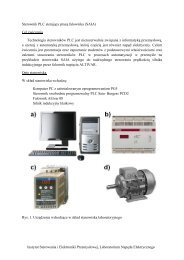


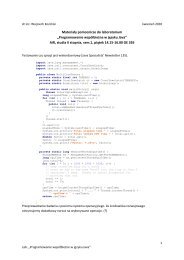


![[TCP] Opis układu - Instytut Sterowania i Elektroniki Przemysłowej ...](https://img.yumpu.com/23535443/1/184x260/tcp-opis-ukladu-instytut-sterowania-i-elektroniki-przemyslowej-.jpg?quality=85)