Robot Mechanisms and Mechanical Devices Illustrated - Profe Saul

www.GetPedia.com

Robot Mechanisms
and Mechanical
Devices Illustrated
Paul E. Sandin
McGraw-Hill
New York | Chicago | San Francisco | Lisbon | London | Madrid
Mexico City | Milan | New Delhi | San Juan | Seoul | Singapore | Sydney | Toronto

Copyright © 2003 by The McGraw-Hill Companies, Inc. All rights reserved. Manufactured in the United States of America.
Except as permitted under the United States Copyright Act of 1976, no part of this publication may be reproduced or distributed
in any form or by any means, or stored in a database or retrieval system, without the prior written permission of the
publisher.
0-07-142928-X
The material in this eBook also appears in the print version of this title: 0-07-141200-X
All trademarks are trademarks of their respective owners. Rather than put a trademark symbol after every occurrence of a
trademarked name, we use names in an editorial fashion only, and to the benefit of the trademark owner, with no intention
of infringement of the trademark. Where such designations appear in this book, they have been printed with initial caps.
McGraw-Hill eBooks are available at special quantity discounts to use as premiums and sales promotions, or for use in corporate
training programs. For more information, please contact George Hoare, Special Sales, at george_hoare@mcgrawhill.com
or (212) 904-4069.
TERMS OF USE
This is a copyrighted work and The McGraw-Hill Companies, Inc. (“McGraw-Hill”) and its licensors reserve all rights in
and to the work. Use of this work is subject to these terms. Except as permitted under the Copyright Act of 1976 and the
right to store and retrieve one copy of the work, you may not decompile, disassemble, reverse engineer, reproduce, modify,
create derivative works based upon, transmit, distribute, disseminate, sell, publish or sublicense the work or any part of it
without McGraw-Hill’s prior consent. You may use the work for your own noncommercial and personal use; any other use
of the work is strictly prohibited. Your right to use the work may be terminated if you fail to comply with these terms.
THE WORK IS PROVIDED “AS IS”. McGRAW-HILL AND ITS LICENSORS MAKE NO GUARANTEES OR WAR-
RANTIES AS TO THE ACCURACY, ADEQUACY OR COMPLETENESS OF OR RESULTS TO BE OBTAINED FROM
USING THE WORK, INCLUDING ANY INFORMATION THAT CAN BE ACCESSED THROUGH THE WORK VIA
HYPERLINK OR OTHERWISE, AND EXPRESSLY DISCLAIM ANY WARRANTY, EXPRESS OR IMPLIED,
INCLUDING BUT NOT LIMITED TO IMPLIED WARRANTIES OF MERCHANTABILITY OR FITNESS FOR A PAR-
TICULAR PURPOSE. McGraw-Hill and its licensors do not warrant or guarantee that the functions contained in the work
will meet your requirements or that its operation will be uninterrupted or error free. Neither McGraw-Hill nor its licensors
shall be liable to you or anyone else for any inaccuracy, error or omission, regardless of cause, in the work or for any damages
resulting therefrom. McGraw-Hill has no responsibility for the content of any information accessed through the work.
Under no circumstances shall McGraw-Hill and/or its licensors be liable for any indirect, incidental, special, punitive, consequential
or similar damages that result from the use of or inability to use the work, even if any of them has been advised
of the possibility of such damages. This limitation of liability shall apply to any claim or cause whatsoever whether such
claim or cause arises in contract, tort or otherwise.
DOI: 10.1036/007142928X

For Vicky, Conor, and Alex

This page intentionally left blank.

For more information about this title, click here.
Contents
Introduction
Acknowledgments
xi
xxxv
Chapter 1 Motor and Motion Control Systems 1
Introduction 3
Merits of Electric Systems 4
Motion Control Classification 5
Closed-Loop System 5
Trapezoidal Velocity Profile 7
Closed-Loop Control Techniques 8
Open-Loop Motion Control Systems 9
Kinds of Controlled Motion 9
Motion Interpolation 10
Computer-Aided Emulation 10
Mechanical Components 11
Electronic System Components 15
Motor Selection 16
Motor Drivers (Amplifiers) 18
Feedback Sensors 19
Installation and Operation of the System 20
Servomotors, Stepper Motors, and Actuators for
Motion Control 20
Permanent-Magnet DC Servomotors 21
Brush-Type PM DC Servomotors 22
Disk-Type PM DC Motors 23
Cup- or Shell-Type PM DC Motors 24
Position Sensing in Brushless Motors 29
Brushless Motor Advantages 30
Brushless DC Motor Disadvantages 31
Characteristics of Brushless Rotary Servomotors 31
Linear Servomotors 31
v
Copyright © 2003 by The McGraw-Hill Companies, Inc. Click here for Terms of Use.

vi
Contents
Commutation 34
Installation of Linear Motors 35
Advantages of Linear vs. Rotary Servomotors 36
Coil Assembly Heat Dissipation 37
Stepper Motors 37
Permanent-Magnet (PM) Stepper Motors 38
Variable Reluctance Stepper Motors 38
Hybrid Stepper Motors 38
Stepper Motor Applications 40
DC and AC Motor Linear Actuators 41
Stepper-Motor Based Linear Actuators 42
Servosystem Feedback Sensors 43
Rotary Encoders 43
Incremental Encoders 44
Absolute Encoders 46
Linear Encoders 47
Magnetic Encoders 48
Resolvers 49
Tachometers 51
Linear Variable Differential Transformers (LVDTs) 53
Linear Velocity Transducers (LVTs) 55
Angular Displacement Transducers (ATDs) 55
Inductosyns 57
Laser Interferometers 57
Precision Multiturn Potentiometers 59
Solenoids and Their Applications 60
Solenoids: An Economical Choice for Linear or Rotary Motion 60
Technical Considerations 62
Open-Frame Solenoids 63
C-Frame Solenoids 63
Box-Frame Solenoids 63
Tubular Solenoids 64
Rotary Solenoids 64
Rotary Actuators 66
Actuator Count 67
Debugging 67
Reliability 68
Cost 68
Chapter 2 Indirect Power Transfer Devices 69
Belts 72

Contents
vii
Flat Belts 73
O-Ring Belts 73
V-Belts 73
Timing Belts 75
Smoother Drive Without Gears 76
Plastic-and-Cable Chain 77
Chain 79
Ladder Chain 80
Roller Chain 80
Rack and Pinion Chain Drive 82
Timing or Silent Chain 82
Friction Drives 83
Cone Drive Needs No Gears Or Pulleys 84
Gears 85
Gear Terminology 87
Gear Dynamics Terminology 88
Gear Classification 88
Worm Gears 90
Worm Gear with Hydrostatic Engagement 90
Controlled Differential Drives 93
Twin-Motor Planetary Gears Provide Safety Plus Dual-Speed 95
Harmonic-Drive Speed Reducers 96
Advantages and Disadvantages 99
Flexible Face-Gears Make Efficient High-Reduction Drives 100
High-Speed Gearheads Improve Small Servo Performance 102
Simplify the Mounting 102
Cost-Effective Addition 104
Chapter 3 Direct Power Transfer Devices 107
Couplings 109
Methods for Coupling Rotating Shafts 110
Ten Universal Shaft Couplings 114
Hooke’s Joints 114
Constant-Velocity Couplings 115
Coupling of Parallel Shafts 117
Ten Different Splined Connections 118
Cylindrical Splines 118
Face Splines 120
Torque Limiters 121
Ten Torque-Limiters 121
One Time Use Torque Limiting 125

viii
Contents
Chapter 4 Wheeled Vehicle Suspensions and Drivetrains 127
Wheeled Mobility Systems 130
Why Not Springs? 130
Shifting the Center of Gravity 131
Wheel Size 134
Three-Wheeled Layouts 136
Four-Wheeled Layouts 141
All-Terrain Vehicle with Self-Righting and Pose Control 144
Six-Wheeled Layouts 150
Eight-Wheeled Layouts 155
Chapter 5 Tracked Vehicle Suspensions and Drive Trains 161
Steering Tracked Vehicles 167
Various Track Construction Methods 168
Track Shapes 171
Track Suspension Systems 174
Track System Layouts 178
One-Track Drive Train 178
Two-Tracked Drive Trains 179
Two-Tracked Drive Trains with Separate Steering Systems 180
Four-Tracked Drive Trains 181
Six-Tracked Drive Trains 184
Chapter 6 Steering History 187
Steering Basics 190
The Next Step Up 193
Chapter 7 Walkers 199
Leg Actuators 202
Leg Geometries 203
Walking Techniques 208
Wave Walking 208
Independent Leg Walking 208
Frame Walking 211
Roller-Walkers 214
Flexible Legs 214

Contents
ix
Chapter 8 Pipe Crawlers and Other Special Cases 217
Horizontal Crawlers 220
Vertical Crawlers 221
Traction Techniques for Vertical Pipe Crawlers 222
Wheeled Vertical Pipe Crawlers 223
Tracked Crawlers 224
Other Pipe Crawlers 224
External Pipe Vehicles 226
Snakes 226
Chapter 9 Comparing Locomotion Methods 227
What Is Mobility? 229
The Mobility System 229
Size 230
Efficiency 231
The Environment 232
Thermal 232
Ground Cover 233
Topography 233
Obstacles 234
Complexity 235
Speed and Cost 235
The Mobility Index Comparison Method 236
The Practical Method 236
Explain All This Using the Algebraic Method 237
Chapter 10 Manipulator Geometries 239
Positioning, Orienting, How Many Degrees of Freedom? 241
E-Chain 243
Slider Crank 243
Arm Geometries 245
Cartesian or Rectangular 246
Cylindrical 247
Polar or Spherical 248
The Wrist 250
Grippers 252
Passive Parallel Jaw Using Cross Tie 255
Passive Capture Joint with Three Degrees of Freedom 256

x
Contents
Industrial Robots 258
Industrial Robot Advantages 259
Trends in Industrial Robots 259
Industrial Robot Characteristics 261
Chapter 11
Proprioceptive and Environmental Sensing
Mechanisms and Devices 263
Industrial Limit Switches 270
Layouts 276
Combination Trip (Sense) and Hard Stop 277
By-Pass Layouts 278
Reversed Bump 279
Bumper Geometries and Suspensions 280
Simple Bumper Suspension Devices 282
Three Link Planar 283
Tension Spring Star 284
Torsion Swing Arm 284
Horizontal Loose Footed Leaf Spring 285
Sliding Front Pivot 286
Suspension Devices to Detect Motions in All Three Planes 287
Conclusion 289
Index 291

Introduction
This book is meant to be interesting, helpful, and educational to hobbyists,
students, educators, and midlevel engineers studying or
designing mobile robots that do real work. It is primarily focused on
mechanisms and devices that relate to vehicles that move around by
themselves and actually do things autonomously, i.e. a robot. Making a
vehicle that can autonomously drive around, both indoors and out,
seems, at first, like a simple thing. Build a chassis, add drive wheels,
steering wheels, a power source (usually batteries), some control code
that includes some navigation and obstacle avoidance routines or some
other way to control it, throw some bump sensors on it, and presto! a
robot.
Unfortunately, soon after these first attempts, the designer will find
the robot getting stuck on what seem to be innocuous objects or bumps,
held captive under a chair or fallen tree trunk, incapable of doing anything
useful, or with a manipulator that crushes every beer can it tries to
pick up. Knowledge of the mechanics of sensors, manipulators, and the
concept of mobility will help reduce these problems. This book provides
that knowledge with the aid of hundreds of sketches showing drive layouts
and manipulator geometries and their work envelope. It discusses
what mobility really is and how to increase it without increasing the size
of the robot, and how the shape of the robot can have a dramatic effect on
its performance. Interspersed throughout the book are unusual mechanisms
and devices, included to entice the reader to think outside the box.
It is my sincere hope that this book will decrease the time it takes to produce
a working robot, reduce the struggles and effort required to achieve
that goal, and, therefore, increase the likelihood that your project will be
a success.
Building, designing, and working with practical mobile robots
requires knowledge in three major engineering fields: mechanical, electrical,
and software. Many books have been written on robots, some
focusing on the complete robot system, others giving a cookbook
approach allowing a novice to take segments of chapters and put together
xi
Copyright © 2003 by The McGraw-Hill Companies, Inc. Click here for Terms of Use.

xii
Introduction
a unique robot. While there are books describing the electric circuits
used in robots, and books that teach the software and control code for
robots, there are few that are focused entirely on the mechanisms and
mechanical devices used in mobile robots.
This book intends to fill the gap in the literature of mobile robots by
containing, in a single reference, complete graphically presented information
on the mechanics of a mobile robot. It is written in laymen’s language
and filled with sketches so novices and those not trained in
mechanical engineering can acquire some understanding of this interesting
field. It also includes clever schemes and mechanisms that mid-level
mechanical engineers should find new and useful. Since mobile robots
are being called on to perform more and more complex and practical
tasks, and many are now carrying one or even two manipulators, this
book has a section on manipulators and grippers for mobile robots. It
shows why a manipulator used on a robot is different in several ways
from a manipulator used in industry.
Autonomous robots place special demands on their mobility system
because of the unstructured and highly varied environment the robot
might drive through, and the fact that even the best sensors are poor in
comparison to a human’s ability to see, feel, and balance. This means the
mobility system of a robot that relies on those sensors will have much
less information about the environment and will encounter obstacles that
it must deal with on its own. In many cases, the microprocessor controlling
the robot will only be telling the mobility system “go over there”
without regard to what lays directly in that path. This forces the mobility
system to be able to handle anything that comes along.
In contrast, a human driver has very acute sensors: eyes for seeing
things and ranging distances, force sensors to sense acceleration, and
balance to sense levelness. A human expects certain things of an automobile’s
(car, truck, jeep, HumVee, etc.) mobility system (wheels, suspension,
and steering) and uses those many and powerful sensors to
guide that mobility system’s efforts to traverse difficult terrain. The
robot’s mobility system must be passively very capable, the car’s mobility
system must feel right to a human.
For these reasons, mobility systems on mobile robots can be both simpler
and more complex than those found in automobiles. For example,
the Ackerman steering system in automobiles is not actually suited for
high mobility. It feels right to a human, and it is well suited to higher
speed travel, but a robot doesn’t care about feeling right, not yet, at least!
The best mobility system for a robot to have is one that effectively
accomplishes the required task, without regard to how well a human
could use it.

Introduction
xiii
There are a few terms specific to mobile robots that must be defined to
avoid confusion. First, the term robot itself has unfortunately come to
have at least three different meanings. In this book, the word robot
means an autonomous or semi-autonomous mobile land vehicle that may
or may not have a manipulator or other device for affecting its environment.
Colin Angle, CEO of iRobot Corp. defines a robot as a mobile
thing with sensors that looks at those sensors and decides on its own
what actions to take.
In the manufacturing industry, however, the word robot means a
reprogrammable stationary manipulator with few, if any sensors, commonly
found in large industrial manufacturing plants. The third common
meaning of robot is a teleoperated vehicle similar to but more sophisticated
than a radio controlled toy car or truck. This form of robot usually
has a microprocessor on it to aid in controlling the vehicle itself, perform
some autonomous or automatic tasks, and aid in controlling the manipulator
if one is onboard.
This book mainly uses the first meaning of robot and focuses on
things useful to making robots, but it also includes several references to
mechanisms useful to both of the other types of robots. Robot and
mobile robot are used interchangeably throughout the book.
Autonomous, in this book, means acting completely independent of any
human input. Therefore, autonomous robot means a self-controlled, selfpowered,
mobile vehicle that makes its own decisions based on inputs
from sensors. There are very few truly autonomous robots, and no
known autonomous robots with manipulators on them whose manipulators
are also autonomous. The more common form of mobile robot today
is semiautonomous, where the robot has some sensors and acts partially
on its own, but there is always a human in the control loop through a
radio link or tether. Another name for this type of control structure is
telerobotic, as opposed to a teleoperated robot, where there are no, or
very few, sensors on the vehicle that it uses to make decisions. Specific
vehicles in this book that do not use sensors to make decisions are
labeled telerobotic or teleoperated to differentiate them from
autonomous robots. It is important to note that the mechanisms and
mechanical devices that are shown in this book can be applied, in their
appropriate category, to almost any vehicle or manipulator whether
autonomous or not.
Another word, which gets a lot of use in the robot world, is mobility.
Mobility is defined in this book as a drive system’s ability to deal with
the effects of heat and ice, ground cover, slopes or staircases, and to
negotiate obstacles. Chapter Nine focuses entirely on comparing drive
systems’ mobility based on a wide range of common obstacles found in

xiv
Introduction
outdoor and indoor environments, some of which can be any size (like
rocks), others that cannot (like stair cases).
I intentionally left out the whole world of hydraulics. While
hydraulic power can be the answer when very compact actuators or
high power density motors are required, it is potentially more dangerous,
and definitely messier, to work with than electrically powered
devices. It is also much less efficient—a real problem for battery powered
robots. There are many texts on hydraulic power and its uses. If
hydraulics is being considered in a design, the reader is referred to Industrial
Fluid Power (4 volumes) 3rd ed., published by Womack Education
Publications.
The designer has powerful tools to aid in the design process beyond
the many tricks, mechanical devices, and techniques shown in this book.
These tools include 3D design tools like SolidWorks and Pro-Engineer
and also new ways to produce prototypes of the mechanisms themselves.
This is commonly called Rapid Prototyping (RP).
NEW PROCESSES EXPAND CHOICES
FOR RAPID PROTOTYPING
New concepts in rapid prototyping (RP) have made it possible to build
many different kinds of 3D prototype models faster and cheaper than by
traditional methods. The 3D models are fashioned automatically from
such materials as plastic or paper, and they can be full size or scaleddown
versions of larger objects. Rapid-prototyping techniques make use
of computer programs derived from computer-aided design (CAD)
drawings of the object. The completed models, like those made by
machines and manual wood carving, make it easier for people to visualize
a new or redesigned product. They can be passed around a conference
table and will be especially valuable during discussions among product
design team members, manufacturing managers, prospective suppliers,
and customers.
At least nine different RP techniques are now available commercially,
and others are still in the development stage. Rapid prototyping models
can be made by the owners of proprietary equipment, or the work can be
contracted out to various RP centers, some of which are owned by the RP
equipment manufacturers. The selection of the most appropriate RP
method for any given modeling application usually depends on the
urgency of the design project, the relative costs of each RP process, and

Introduction
xv
the anticipated time and cost savings RP will offer over conventional
model-making practice. New and improved RP methods are being introduced
regularly, so the RP field is in a state of change, expanding the
range of designer choices.
Three-dimensional models can be made accurately enough by RP
methods to evaluate the design process and eliminate interference fits or
dimensioning errors before production tooling is ordered. If design flaws
or omissions are discovered, changes can be made in the source CAD
program and a replacement model can be produced quickly to verify that
the corrections or improvements have been made. Finished models are
useful in evaluations of the form, fit, and function of the product design
and for organizing the necessary tooling, manufacturing, or even casting
processes.
Most of the RP technologies are additive; that is, the model is made
automatically by building up contoured laminations sequentially from
materials such as photopolymers, extruded or beaded plastic, and even
paper until they reach the desired height. These processes can be used to
form internal cavities, overhangs, and complex convoluted geometries as
well as simple planar or curved shapes. By contrast, a subtractive RP
process involves milling the model from a block of soft material, typically
plastic or aluminum, on a computer-controlled milling machine
with commands from a CAD-derived program.
In the additive RP processes, photopolymer systems are based on successively
depositing thin layers of a liquid resin, which are then solidified
by exposure to a specific wavelengths of light. Thermoplastic systems
are based on procedures for successively melting and fusing solid
filaments or beads of wax or plastic in layers, which harden in the air to
form the finished object. Some systems form layers by applying adhesives
or binders to materials such as paper, plastic powder, or coated
ceramic beads to bond them.
The first commercial RP process introduced was stereolithography in
1987, followed by a succession of others. Most of the commercial RP
processes are now available in Europe and Japan as well as the United
States. They have become multinational businesses through branch
offices, affiliates, and franchises.
Each of the RP processes focuses on specific market segments, taking
into account their requirements for model size, durability, fabrication
speed, and finish in the light of anticipated economic benefits and cost.
Some processes are not effective in making large models, and each
process results in a model with a different finish. This introduces an economic
tradeoff of higher price for smoother surfaces versus additional
cost and labor of manual or machine finishing by sanding or polishing.

xvi
Introduction
Rapid prototyping is now also seen as an integral part of the even
larger but not well defined rapid tooling (RT) market. Concept modeling
addresses the early stages of the design process, whereas RT concentrates
on production tooling or mold making.
Some concept modeling equipment, also called 3D or office printers,
are self-contained desktop or benchtop manufacturing units small
enough and inexpensive enough to permit prototype fabrication to be
done in an office environment. These units include provision for the containment
or venting of any smoke or noxious chemical vapors that will
be released during the model’s fabrication.
Computer-Aided Design Preparation
The RP process begins when the object is drawn on the screen of a CAD
workstation or personal computer to provide the digital data base. Then,
in a post-design data processing step, computer software slices the object
mathematically into a finite number of horizontal layers in generating an
STL (Solid Transfer Language) file. The thickness of the “slices” can
range from 0.0025 to 0.5 in. (0.06 to 13 mm) depending on the RP
process selected. The STL file is then converted to a file that is compatible
with the specific 3D “printer” or processor that will construct the
model.
The digitized data then guides a laser, X-Y table, optics, or other
apparatus that actually builds the model in a process comparable to
building a high-rise building one story at a time. Slice thickness might
have to be modified in some RP processes during model building to
compensate for material shrinkage.
Prototyping Choices
All of the commercial RP methods depend on computers, but four of
them depend on laser beams to cut or fuse each lamination, or provide
enough heat to sinter or melt certain kinds of materials. The four
processes that make use of lasers are Directed-Light Fabrication (DLF),
Laminated-Object Manufacturing (LOM), Selective Laser Sintering
(SLS), and Stereolithography (SL); the five processes that do not require
lasers are Ballistic Particle Manufacturing (BPM), Direct-Shell
Production Casting (DSPC), Fused-Deposition Modeling (FDM), Solid-
Ground Curing (SGC), and 3D Printing (3DP).

Introduction
xvii
Stereolithography (SL)
The stereolithographic (SL) process is performed on the equipment
shown in Figure 1. The movable platform on which the 3D model is
formed is initially immersed in a vat of liquid photopolymer resin to a
level just below its surface so that a thin layer of the resin covers it. The
SL equipment is located in a sealed chamber to prevent the escape of
fumes from the resin vat.
The resin changes from a liquid to a solid when exposed to the ultraviolet
(UV) light from a low-power, highly focused laser. The UV laser
beam is focused on an X-Y mirror in a computer-controlled beam-shaping
and scanning system so that it draws the outline of the lowest crosssection
layer of the object being built on the film of photopolymer resin.
After the first layer is completely traced, the laser is then directed to
scan the traced areas of resin to solidify the model’s first cross section.
The laser beam can harden the layer down to a depth of 0.0025 to 0.0300
in. (0.06 to 0.8 mm). The laser beam scans at speeds up to 350 in./s (890
cm/s). The photopolymer not scanned by the laser beam remains a liquid.
In general, the thinner the resin film (slice thickness), the higher the
resolution or more refined the finish of the completed model. When
model surface finish is important, layer thicknesses are set for 0.0050 in.
(0.13 mm) or less.
The table is then submerged under computer control to the specified
depth so that the next layer of liquid polymer flows over the first hardened
layer. The tracing, hardening, and recoating steps are repeated,
layer-by-layer, until the complete 3D model is built on the platform
within the resin vat.
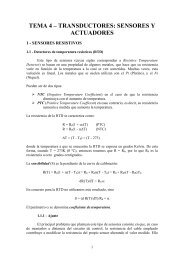
Figure 1 Stereolithography (SL):
A computer-controlled
neon–helium ultraviolet light
(UV)–emitting laser outlines each
layer of a 3D model in a thin liquid
film of UV-curable photopolymer
on a platform submerged a
vat of the resin. The laser then
scans the outlined area to solidify
the layer, or “slice.” The platform
is then lowered into the liquid to
a depth equal to layer thickness,
and the process is repeated for
each layer until the 3D model is
complete. Photopolymer not
exposed to UV remains liquid.
The model is them removed for
finishing.

xviii
Introduction
Because the photopolymer used in the SL process tends to curl or sag
as it cures, models with overhangs or unsupported horizontal sections
must be reinforced with supporting structures: walls, gussets, or
columns. Without support, parts of the model can sag or break off before
the polymer has fully set. Provision for forming these supports is
included in the digitized fabrication data. Each scan of the laser forms
support layers where necessary while forming the layers of the model.
When model fabrication is complete, it is raised from the polymer vat
and resin is allowed to drain off; any excess can be removed manually
from the model’s surfaces. The SL process leaves the model only partially
polymerized, with only about half of its fully cured strength. The
model is then finally cured by exposing it to intense UV light in the
enclosed chamber of post-curing apparatus (PCA). The UV completes
the hardening or curing of the liquid polymer by linking its molecules in
chainlike formations. As a final step, any supports that were required are
removed, and the model’s surfaces are sanded or polished. Polymers
such as urethane acrylate resins can be milled, drilled, bored, and tapped,
and their outer surfaces can be polished, painted, or coated with sprayedon
metal.
The liquid SL photopolymers are similar to the photosensitive UVcurable
polymers used to form masks on semiconductor wafers for etching
and plating features on integrated circuits. Resins can be formulated
to solidify under either UV or visible light.
The SL process was the first to gain commercial acceptance, and it
still accounts for the largest base of installed RP systems. 3D Systems of
Valencia, California, is a company that manufactures stereolithography
equipment for its proprietary SLA process. It offers the ThermoJet Solid
Object Printer. The SLA process can build a model within a volume
measuring 10 × 7.5 × 8 in. (25 × 19 × 20 cm). It also offers the SLA 7000
system, which can form objects within a volume of 20 × 20 × 23.62 in.
(51 × 51 × 60 cm). Aaroflex, Inc. of Fairfax, Virginia, manufactures the
Aacura 22 solid-state SL system and operates AIM, an RP manufacturing
service.
Solid Ground Curing (SGC)
Solid ground curing (SGC) (or the “solider process”) is a multistep inline
process that is diagrammed in Figure 2. It begins when a photomask
for the first layer of the 3D model is generated by the equipment shown
at the far left. An electron gun writes a charge pattern of the photomask
on a clear glass plate, and opaque toner is transferred electrostatically to
the plate to form the photolithographic pattern in a xerographic process.

Introduction
xix
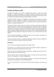
Figure 2 Solid Ground Curing (SGC): First, a photomask is generated on a glass plate by
a xerographic process. Liquid photopolymer is applied to the work platform to form a
layer, and the platform is moved under the photomask and a strong UV source that
defines and hardens the layer. The platform then moves to a station for excess polymer
removal before wax is applied over the hardened layer to fill in margins and spaces. After
the wax is cooled, excess polymer and wax are milled off to form the first “slice.” The first
photomask is erased, and a second mask is formed on the same glass plate. Masking and
layer formation are repeated with the platform being lowered and moved back and forth
under the stations until the 3D model is complete. The wax is then removed by heating
or immersion in a hot water bath to release the prototype.
The photomask is then moved to the exposure station, where it is aligned
over a work platform and under a collimated UV lamp.
Model building begins when the work platform is moved to the right
to a resin application station where a thin layer of photopolymer resin is
applied to the top surface of the work platform and wiped to the desired
thickness. The platform is then moved left to the exposure station, where
the UV lamp is then turned on and a shutter is opened for a few seconds
to expose the resin layer to the mask pattern. Because the UV light is so
intense, the layer is fully cured and no secondary curing is needed.
The platform is then moved back to the right to the wiper station,
where all of resin that was not exposed to UV is removed and discarded.
The platform then moves right again to the wax application station,
where melted wax is applied and spread into the cavities left by the
removal of the uncured resin. The wax is hardened at the next station by
pressing it against a cooling plate. After that, the platform is moved right
again to the milling station, where the resin and wax layer are milled to a
precise thickness. The platform piece is then returned to the resin application
station, where it is lowered a depth equal to the thickness of the
next layer and more resin is applied.

xx
Introduction
Meanwhile, the opaque toner has been removed from the glass mask
and a new mask for the next layer is generated on the same plate. The
complete cycle is repeated, and this will continue until the 3D model
encased in the wax matrix is completed. This matrix supports any overhangs
or undercuts, so extra support structures are not needed.
After the prototype is removed from the process equipment, the wax is
either melted away or dissolved in a washing chamber similar to a dishwasher.
The surface of the 3D model is then sanded or polished by other
methods.
The SGC process is similar to drop on demand inkjet plotting, a
method that relies on a dual inkjet subsystem that travels on a precision
X-Y drive carriage and deposits both thermoplastic and wax materials
onto the build platform under CAD program control. The drive carriage
also energizes a flatbed milling subsystem for obtaining the precise vertical
height of each layer and the overall object by milling off the excess
material.
Cubital America Inc., Troy, Michigan, offers the Solider 4600/5600
equipment for building prototypes with the SGC process.
Selective Laser Sintering (SLS)
Selective laser sintering (SLS) is another RP process similar to stereolithography
(SL). It creates 3D models from plastic, metal, or ceramic
powders with heat generated by a carbon dioxide infrared (IR)–emitting
laser, as shown in Figure 3. The prototype is fabricated in a cylinder with
a piston, which acts as a moving platform, and it is positioned next to a
cylinder filled with preheated powder. A piston within the powder delivery
system rises to eject powder, which is spread by a roller over the top
of the build cylinder. Just before it is applied, the powder is heated further
until its temperature is just below its melting point
When the laser beam scans the thin layer of powder under the control
of the optical scanner system, it raises the temperature of the powder
even further until it melts or sinters and flows together to form a solid
layer in a pattern obtained from the CAD data.
As in other RP processes, the piston or supporting platform is lowered
upon completion of each layer and the roller spreads the next layer of
powder over the previously deposited layer. The process is repeated, with
each layer being fused to the underlying layer, until the 3D prototype is
completed.
The unsintered powder is brushed away and the part removed. No
final curing is required, but because the objects are sintered they are
porous. Wax, for example, can be applied to the inner and outer porous

Introduction
xxi
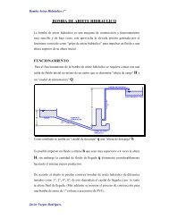
Figure 3 Selective Laser Sintering (SLS): Loose plastic powder from a reservoir is distributed
by roller over the surface of piston in a build cylinder positioned at a depth below
the table equal to the thickness of a single layer. The powder layer is then scanned by a
computer-controlled carbon dioxide infrared laser that defines the layer and melts the
powder to solidify it. The cylinder is again lowered, more powder is added, and the
process is repeated so that each new layer bonds to the previous one until the 3D model
is completed. It is then removed and finished. All unbonded plastic powder can be
reused.
surfaces, and it can be smoothed by various manual or machine grinding
or melting processes. No supports are required in SLS because overhangs
and undercuts are supported by the compressed unfused powder
within the build cylinder.
Many different powdered materials have been used in the SLS
process, including polycarbonate, nylon, and investment casting wax.
Polymer-coated metal powder is also being studied as an alternative. One
advantage of the SLS process is that materials such as polycarbonate and
nylon are strong and stable enough to permit the model to be used in limited
functional and environmental testing. The prototypes can also serve
as molds or patterns for casting parts.
SLS process equipment is enclosed in a nitrogen-filled chamber that is
sealed and maintained at a temperature just below the melting point of
the powder. The nitrogen prevents an explosion that could be caused by
the rapid oxidation of the powder.
The SLS process was developed at the University of Texas at Austin,
and it has been licensed by the DTM Corporation of Austin, Texas. The
company makes a Sinterstation 2500plus. Another company participating
in SLS is EOS GmbH of Germany.

xxii
Introduction
Laminated-Object Manufacturing (LOM)
The Laminated-Object Manufacturing (LOM) process, diagrammed in
Figure 4, forms 3D models by cutting, stacking, and bonding successive
layers of paper coated with heat-activated adhesive. The carbon-dioxide
laser beam, directed by an optical system under CAD data control, cuts
cross-sectional outlines of the prototype in the layers of paper, which are
bonded to previous layers to become the prototype.
The paper that forms the bottom layer is unwound from a supply roll
and pulled across the movable platform. The laser beam cuts the outline
of each lamination and cross-hatches the waste material within and
around the lamination to make it easier to remove after the prototype is
completed. The outer waste material web from each lamination is continuously
removed by a take-up roll. Finally, a heated roller applies pressure
to bond the adhesive coating on each layer cut from the paper to the
previous layer.
A new layer of paper is then pulled from a roll into position over the
previous layer, and the cutting, cross hatching, web removal, and bonding
procedure is repeated until the model is completed. When all the layers
have been cut and bonded, the excess cross-hatched material in the
Figure 4 Laminated Object Manufacturing (LOM): Adhesive-backed paper is fed across
an elevator platform and a computer-controlled carbon dioxide infrared-emitting laser
cuts the outline of a layer of the 3D model and cross-hatches the unused paper. As more
paper is fed across the first layer, the laser cuts the outline and a heated roller bonds the
adhesive of the second layer to the first layer. When all the layers have been cut and
bonded, the cross-hatched material is removed to expose the finished model. The complete
model can then be sealed and finished.

Introduction
xxiii
form of stacked segments is removed to reveal the finished 3D model.
The models made by the LOM have woodlike finishes that can be sanded
or polished before being sealed and painted.
Using inexpensive, solid-sheet materials makes the 3D LOM models
more resistant to deformity and less expensive to produce than models
made by other processes, its developers say. These models can be used
directly as patterns for investment and sand casting, and as forms for silicone
molds. The objects made by LOM can be larger than those made
by most other RP processes—up to 30 × 20 × 20 in. (75 × 50 × 50 cm).
The LOM process is limited by the ability of the laser to cut through
the generally thicker lamination materials and the additional work that
must be done to seal and finish the model’s inner and outer surfaces.
Moreover, the laser cutting process burns the paper, forming smoke that
must be removed from the equipment and room where the LOM process
is performed.
Helysys Corporation, Torrance, California, manufactures the LOM-
2030H LOM equipment. Alternatives to paper including sheet plastic
and ceramic and metal-powder-coated tapes have been developed.
Other companies offering equipment for building prototypes from
paper laminations are the Schroff Development Corporation, Mission,
Kansas, and CAM-LEM, Inc. Schroff manufactures the JP System 5 to
permit desktop rapid prototyping.
Fused Deposition Modeling (FDM)
The Fused Deposition Modeling (FDM) process, diagrammed in Figure 5,
forms prototypes from melted thermoplastic filament. This filament,
with a diameter of 0.070 in. (1.78 mm), is fed into a temperaturecontrolled
FDM extrusion head where it is heated to a semi-liquid state.
It is then extruded and deposited in ultrathin, precise layers on a fixtureless
platform under X-Y computer control. Successive laminations ranging
in thickness from 0.002 to 0.030 in. (0.05 to 0.76 mm) with wall
thicknesses of 0.010 to 0.125 in. (0.25 to 3.1 mm) adhere to each by thermal
fusion to form the 3D model.
Structures needed to support overhanging or fragile structures in FDM
modeling must be designed into the CAD data file and fabricated as part
of the model. These supports can easily be removed in a later secondary
operation.
All components of FDM systems are contained within temperaturecontrolled
enclosures. Four different kinds of inert, nontoxic filament
materials are being used in FDM: ABS polymer (acrylonitrile butadiene
styrene), high-impact-strength ABS (ABSi), investment casting wax, and

xxiv
Introduction
Figure 5 Fused Deposition Modeling (FDM): Filaments of thermoplastic are unwound
from a spool, passed through a heated extrusion nozzle mounted on a computercontrolled
X-Y table, and deposited on the fixtureless platform. The 3D model is formed
as the nozzle extruding the heated filament is moved over the platform. The hot filament
bonds to the layer below it and hardens. This laserless process can be used to form thinwalled,
contoured objects for use as concept models or molds for investment casting. The
completed object is removed and smoothed to improve its finish.
elastomer. These materials melt at temperatures between 180 and 220ºF
(82 and 104ºC).
FDM is a proprietary process developed by Stratasys, Eden Prairie,
Minnesota. The company offers four different systems. Its Genisys
benchtop 3D printer has a build volume as large as 8 × 8 × 8 in. (20 × 20
× 20 cm), and it prints models from square polyester wafers that are
stacked in cassettes. The material is heated and extruded through a 0.01-
in. (0.25-mm)–diameter hole at a controlled rate. The models are built on
a metallic substrate that rests on a table. Stratasys also offers four systems
that use spooled material. The FDM2000, another benchtop system,
builds parts up to 10 in 3 (164 cm 3 ) while the FDM3000, a floorstanding
system, builds parts up to 10 × 10 × 16 in. (26 × 26 × 41 cm).
Two other floor-standing systems are the FDM 8000, which builds
models up to 18 × 18 × 24 in. (46 × 46 × 61 cm), and the FDM Quantum
system, which builds models up to 24 × 20 × 24 in. (61 × 51 × 61 cm).
All of these systems can be used in an office environment.
Stratasys offers two options for forming and removing supports: a
breakaway support system and a water-soluble support system. The

Introduction
xxv
water-soluble supports are formed by a separate extrusion head, and they
can be washed away after the model is complete.
Three-Dimensional Printing (3DP)
The Three-Dimensional Printing (3DP) or inkjet printing process, diagrammed
in Figure 6, is similar to Selective Laser Sintering (SLS)
except that a multichannel inkjet head and liquid adhesive supply
replaces the laser. The powder supply cylinder is filled with starch and
cellulose powder, which is delivered to the work platform by elevating a
delivery piston. A roller rolls a single layer of powder from the powder
cylinder to the upper surface of a piston within a build cylinder. A multichannel
inkjet head sprays a water-based liquid adhesive onto the surface
of the powder to bond it in the shape of a horizontal layer of the model.
In successive steps, the build piston is lowered a distance equal to the
thickness of one layer while the powder delivery piston pushes up fresh
powder, which the roller spreads over the previous layer on the build pis-
Figure 6 Three-Dimensional Printing (3DP): Plastic powder from a reservoir is spread
across a work surface by roller onto a piston of the build cylinder recessed below a table
to a depth equal to one layer thickness in the 3DP process. Liquid adhesive is then
sprayed on the powder to form the contours of the layer. The piston is lowered again,
another layer of powder is applied, and more adhesive is sprayed, bonding that layer to
the previous one. This procedure is repeated until the 3D model is complete. It is then
removed and finished.

xxvi
Introduction
ton. This process is repeated until the 3D model is complete. Any loose
excess powder is brushed away, and wax is coated on the inner and outer
surfaces of the model to improve its strength.
The 3DP process was developed at the Three-Dimensional Printing
Laboratory at the Massachusetts Institute of Technology, and it has been
licensed to several companies. One of those firms, the Z Corporation of
Somerville, Massachusetts, uses the original MIT process to form 3D
models. It also offers the Z402 3D modeler. Soligen Technologies has
modified the 3DP process to make ceramic molds for investment casting.
Other companies are using the process to manufacture implantable
drugs, make metal tools, and manufacture ceramic filters.
Direct-Shell Production Casting (DSPC)
The Direct Shell Production Casting (DSPC) process, diagrammed in
Figure 7, is similar to the 3DP process except that it is focused on forming
molds or shells rather than 3D models. Consequently, the actual 3D
model or prototype must be produced by a later casting process. As in the
3DP process, DSPC begins with a CAD file of the desired prototype.
Figure 7 Direct Shell Production Casting (DSPC): Ceramic molds rather than 3D models
are made by DSPC in a layering process similar to other RP methods. Ceramic powder is
spread by roller over the surface of a movable piston that is recessed to the depth of a single
layer. Then a binder is sprayed on the ceramic powder under computer control. The
next layer is bonded to the first by the binder. When all of the layers are complete, the
bonded ceramic shell is removed and fired to form a durable mold suitable for use in metal
casting. The mold can be used to cast a prototype. The DSPC process is considered to be
an RP method because it can make molds faster and cheaper than conventional methods.

Introduction
xxvii
Two specialized kinds of equipment are needed for DSPC: a dedicated
computer called a shell-design unit (SDU) and a shell- or moldprocessing
unit (SPU). The CAD file is loaded into the SDU to generate
the data needed to define the mold. SDU software also modifies the original
design dimensions in the CAD file to compensate for ceramic
shrinkage. This software can also add fillets and delete such features as
holes or keyways that must be machined after the prototype is cast.
The movable platform in DSPC is the piston within the build cylinder.
It is lowered to a depth below the rim of the build cylinder equal to the
thickness of each layer. Then a thin layer of fine aluminum oxide (alumina)
powder is spread by roller over the platform, and a fine jet of colloidal
silica is sprayed precisely onto the powder surface to bond it in the
shape of a single mold layer. The piston is then lowered for the next layer
and the complete process is repeated until all layers have been formed,
completing the entire 3D shell. The excess powder is then removed, and
the mold is fired to convert the bonded powder to monolithic ceramic.
After the mold has cooled, it is strong enough to withstand molten
metal and can function like a conventional investment-casting mold.
After the molten metal has cooled, the ceramic shell and any cores or
gating are broken away from the prototype. The casting can then be finished
by any of the methods usually used on metal castings.
DSPC is a proprietary process of Soligen Technologies, Northridge,
California. The company also offers a custom mold manufacturing service.
Ballistic Particle Manufacturing (BPM)
There are several different names for the Ballistic Particle Manufacturing
(BPM) process, diagrammed in Figure 8. Variations of it are
also called inkjet methods. The molten plastic used to form the model
and the hot wax for supporting overhangs or indentations are kept in
heated tanks above the build station and delivered to computercontrolled
jet heads through thermally insulated tubing. The jet heads
squirt tiny droplets of the materials on the work platform as it is moved
by an X-Y table in the pattern needed to form each layer of the 3D
object. The droplets are deposited only where directed, and they harden
rapidly as they leave the jet heads. A milling cutter is passed over the
layer to mill it to a uniform thickness. Particles that are removed by the
cutter are vacuumed away and deposited in a collector.
Nozzle operation is monitored carefully by a separate fault-detection
system. After each layer has been deposited, a stripe of each material is
deposited on a narrow strip of paper for thickness measurement by opti-

xxviii
Introduction
Figure 8 Ballistic Particle Manufacturing (BPM): Heated plastic and wax are deposited
on a movable work platform by a computer-controlled X-Y table to form each layer. After
each layer is deposited, it is milled to a precise thickness. The platform is lowered and the
next layer is applied. This procedure is repeated until the 3D model is completed. A fault
detection system determines the quality and thickness of the wax and plastic layers and
directs rework if a fault is found. The supporting wax is removed from the 3D model by
heating or immersion in a hot liquid bath.
cal detectors. If the layer meets specifications, the work platform is lowered
a distance equal to the required layer thickness and the next layer is
deposited. However, if a clot is detected in either nozzle, a jet cleaning
cycle is initiated to clear it. Then the faulty layer is milled off and that
layer is redeposited. After the 3D model is completed, the wax material
is either melted from the object by radiant heat or dissolved away in a hot
water wash.
The BPM system is capable of producing objects with fine finishes,
but the process is slow. With this RP method, a slower process that yields
a 3D model with a superior finish is traded off against faster processes
that require later manual finishing.
The version of the BPM system shown in Figure 8 is called Drop on
Demand Inkjet Plotting by Sanders Prototype Inc, Merrimac, New
Hampshire. It offers the ModelMaker II processing equipment, which
produces 3D models with this method. AeroMet Corporation builds titanium
parts directly from CAD renderings by fusing titanium powder
with an 18-kW carbon dioxide laser, and 3D Systems of Valencia,

Introduction
xxix
California, produces a line of inkjet printers that feature multiple jets to
speed up the modeling process.
Directed Light Fabrication (DLF)
The Directed Light Fabrication (DLF) process, diagrammed in Figure 9,
uses a neodymium YAG (Nd:YAG) laser to fuse powdered metals to
build 3D models that are more durable than models made from paper or
plastics. The metal powders can be finely milled 300 and 400 series
stainless steel, tungsten, nickel aluminides, molybdenum disilicide, copper,
and aluminum. The technique is also called Direct-Metal Fusing,
Laser Sintering, and Laser Engineered Net Shaping (LENS).
The laser beam under X-Y computer control fuses the metal powder
fed from a nozzle to form dense 3D objects whose dimensions are said to
be within a few thousandths of an inch of the desired design tolerance.
DLF is an outgrowth of nuclear weapons research at the Los Alamos
National Laboratory (LANL), Los Alamos, New Mexico, and it is still in
the development stage. The laboratory has been experimenting with the
Figure 9 Directed Light Fabrication (DLF): Fine metal powder is distributed on an X-Y
work platform that is rotated under computer control beneath the beam of a neodymium
YAG laser. The heat from the laser beam melts the metal powder to form thin layers of a
3D model or prototype. By repeating this process, the layers are built up and bonded to
the previous layers to form more durable 3D objects than can be made from plastic.
Powdered aluminum, copper, stainless steel, and other metals have been fused to make
prototypes as well as practical tools or parts that are furnace-fired to increase their bond
strength.

xxx
Introduction
laser fusing of ceramic powders to fabricate parts as an alternative to the
use of metal powders. A system that would regulate and mix metal powder
to modify the properties of the prototype is also being investigated.
Optomec Design Company, Albuquerque, New Mexico, has
announced that direct fusing of metal powder by laser in its LENS
process is being performed commercially. Protypes made by this method
have proven to be durable and they have shown close dimensional tolerances.
Research and Development in RP
Many different RP techniques are still in the experimental stage and have
not yet achieved commercial status. At the same time, practical commercial
processes have been improved. Information about this research has
been announced by the laboratories doing the work, and some of the
research is described in patents. This discussion is limited to two techniques,
SDM and Mold SDM, that have shown commercial promise.
Shape Deposition Manufacturing (SDM)
The Shape Deposition Manufacturing (SDM) process, developed at the
SDM Laboratory of Carnegie Mellon University, Pittsburgh,
Pennsylvania, produces functional metal prototypes directly from CAD
data. This process, diagrammed in Figure 10, forms successive layers of
metal on a platform without masking, and is also called solid free- form
(SFF) fabrication. It uses hard metals to form more rugged prototypes
that are then accurately machined under computer control during the
process.
The first steps in manufacturing a part by SDM are to reorganize or
destructure the CAD data into slices or layers of optimum thickness that
will maintain the correct 3D contours of the outer surfaces of the part and
then decide on the sequence for depositing the primary and supporting
materials to build the object.
The primary metal for the first layer is deposited by a process called
microcasting at the deposition station, Figure 10(a). The work is then
moved to a machining station (b), where a computer-controlled milling
machine or grinder removes deposited metal to shape the first layer of
the part. Next, the work is moved to a stress-relief station (c), where it is
shot- peened to relieve stresses that have built up in the layer. The work
is then transferred back to the deposition station (a) for simultaneous
deposition of primary metal for the next layer and sacrificial support

Introduction
xxxi
Figure 10 Shape Deposition Manufacturing (SDM): Functional metal parts or tools can
be formed in layers by repeating three basic steps repetitively until the part is completed.
Hot metal droplets of both primary and sacrificial support material form layers by a thermal
metal spraying technique (a). They retain their heat long enough to remelt the
underlying metal on impact to form strong metallurgical interlayer bonds. Each layer is
machined under computer control (b) and shot-peened (c) to relieve stress buildup
before the work is returned for deposition of the next layer. The sacrificial metal supports
any undercut features. When deposition of all layers is complete, the sacrificial metal is
removed by acid etching to release the completed part.
metal. The support material protects the part layers from the deposition
steps that follow, stabilizes the layer for further machining operations,
and provides a flat surface for milling the next layer. This SDM cycle is
repeated until the part is finished, and then the sacrificial metal is etched
away with acid. One combination of metals that has been successful in
SDM is stainless steel for forming the prototype and copper for forming
the support structure
The SDM Laboratory investigated many thermal techniques for
depositing high-quality metals, including thermal spraying and plasma
or laser welding, before it decided on microcasting, a compromise
between these two techniques that provided better results than either
technique by itself. The metal droplets in microcasting are large enough
(1 to 3 mm in diameter) to retain their heat longer than the 50-mm
droplets formed by conventional thermal spraying. The larger droplets
remain molten and retain their heat long enough so that when they
impact the metal surfaces they remelt them to form a strong metallurgical
interlayer bond. This process overcame the low adhesion and low
mechanical strength problems encountered with conventional thermal
metal spraying. Weld-based deposition easily remelted the substrate

xxxii
Introduction
material to form metallurgical bonds, but the larger amount of heat transferred
tended to warp the substrate or delaminate it.
The SDM laboratory has produced custom-made functional mechanical
parts and has embedded prefabricated mechanical parts, electronic
components, electronic circuits, and sensors in the metal layers during
the SDM process. It has also made custom tools such as injection molds
with internal cooling pipes and metal heat sinks with embedded copper
pipes for heat redistribution.
Mold SDM
The Rapid Prototyping Laboratory at Stanford University, Palo Alto,
California, has developed its own version of SDM, called Mold SDM,
for building layered molds for casting ceramics and polymers. Mold
SDM, as diagrammed in Figure 11, uses wax to form the molds. The wax
occupies the same position as the sacrificial support metal in SDM, and
water-soluble photopolymer sacrificial support material occupies and
supports the mold cavity. The photopolymer corresponds to the primary
metal deposited to form the finished part in SDM. No machining is performed
in this process.
The first step in the Mold SDM process begins with the decomposition
of CAD mold data into layers of optimum thickness, which depends
on the complexity and contours of the mold. The actual processing
begins at Figure 11(a), which shows the results of repetitive cycles of the
deposition of wax for the mold and sacrificial photopolymer in each
layer to occupy the mold cavity and support it. The polymer is hardened
by an ultraviolet (UV) source. After the mold and support structures are
built up, the work is moved to a station (b) where the photopolymer is
removed by dissolving it in water. This exposes the wax mold cavity into
which the final part material is cast. It can be any compatible castable
material. For example, ceramic parts can be formed by pouring a gelcasting
ceramic slurry into the wax mold (c) and then curing the slurry.
The wax mold is then removed (d) by melting it, releasing the “green”
ceramic part for furnace firing. In step (e), after firing, the vents and
sprues are removed as the final step.
Mold SDM has been expanded into making parts from a variety of
polymer materials, and it has also been used to make preassembled
mechanisms, both in polymer and ceramic materials.
For the designer just getting started in the wonderful world of mobile
robots, it is suggested s/he follow the adage “prototype early, prototype
often.” This old design philosophy is far easier to use with the aid of RP
tools. A simpler, cheaper, and more basic method, though, is to use

Introduction
xxxiii
Figure 11 Mold Shape Deposition Manufacturing (MSDM): Casting molds can be
formed in successive layers: Wax for the mold and water-soluble photopolymer to support
the cavity are deposited in a repetitive cycle to build the mold in layers whose thickness
and number depend on the mold’s shape (a). UV energy solidifies the photopolymer.
The photopolymer support material is removed by soaking it in hot water (b). Materials
such as polymers and ceramics can be cast in the wax mold. For ceramic parts, a gelcasting
ceramic slurry is poured into the mold to form green ceramic parts, which are then
cured (c). The wax mold is then removed by heat or a hot liquid bath and the green
ceramic part released (d). After furnace firing (e) any vents and sprues are removed.
Popsicle sticks, crazy glue, hot glue, shirt cardboard, packing tape, clay,
or one of the many construction toy sets, etc. Fast, cheap, and surprisingly
useful information on the effectiveness of whatever concept has
been dreamed up can be achieved with very simple prototypes. There’s
nothing like holding the thing in your hand, even in a crude form, to see
if it has any chance of working as originally conceived.
Robots can be very complicated in final form, especially those that do
real work without aid of humans. Start simple and test ideas one at a time,
then assemble those pieces into subassemblies and test those. Learn as
much as possible about the actual obstacles that might be found in the
environment for which the robot is destined. Design the mobility system
to handle more difficult terrain because there will always be obstacles that
will cause problems even in what appears to be a simple environment.
Learn as much as possible about the required task, and design the manipulator
and end effector to be only as complex as will accomplish that task.
Trial and error is the best method in many fields of design, and is
especially so for robots. Prototype early, prototype often, and test everything.
Mobile robots are inherently complex devices with many interactions
within themselves and with their environment. The result of the
effort, though, is exciting, fun, and rewarding. There is nothing like seeing
an autonomous robot happily driving around, doing some useful task
completely on its own.

This page intentionally left blank.

Acknowledgments
This book would not even have been considered and would never have
been completed without the encouragement and support of my loving
wife, Victoria. Thank you so much.
In addition to the support of my wife, I would like to thank Joe Jones
for his input, criticism, and support. Thank you for putting up with my
many questions. Thanks also goes to Lee Sword, Chi Won, Tim Ohm,
and Scott Miller for input on many of the ideas and layouts. The process
of writing this book was made much easier by iRobot allowing me to use
their office machines. And, lastly, thanks to my extended family, especially
my Dad and Jenny for their encouragement and patience.
xxxv
Copyright © 2003 by The McGraw-Hill Companies, Inc. Click here for Terms of Use.

This page intentionally left blank.

Chapter 1
Motor and Motion
Control Systems
Copyright © 2003 by The McGraw-Hill Companies, Inc. Click here for Terms of Use.

This page intentionally left blank.

INTRODUCTION
A modern motion control system typically consists of a motion controller,
a motor drive or amplifier, an electric motor, and feedback sensors.
The system might also contain other components such as one or
more belt-, ballscrew-, or leadscrew-driven linear guides or axis stages.
A motion controller today can be a standalone programmable controller,
a personal computer containing a motion control card, or a programmable
logic controller (PLC).
All of the components of a motion control system must work together
seamlessly to perform their assigned functions. Their selection must be
based on both engineering and economic considerations. Figure 1-1
illustrates a typical multiaxis X-Y-Z motion platform that includes the
three linear axes required to move a load, tool, or end effector precisely
through three degrees of freedom. With additional mechanical or electro-
Figure 1-1 This multiaxis X-Y-Z
motion platform is an example of
a motion control system.
3

4 Chapter 1 Motor and Motion Control Systems
Figure 1-2 The right-handed
coordinate system showing six
degrees of freedom.
mechanical components on each axis, rotation about the three axes can
provide up to six degrees of freedom, as shown in Figure 1-2.
Motion control systems today can be found in such diverse applications
as materials handling equipment, machine tool centers, chemical
and pharmaceutical process lines, inspection stations, robots, and injection
molding machines.
Merits of Electric Systems
Most motion control systems today are powered by electric motors
rather than hydraulic or pneumatic motors or actuators because of the
many benefits they offer:
• More precise load or tool positioning, resulting in fewer product or
process defects and lower material costs.
• Quicker changeovers for higher flexibility and easier product customizing.
• Increased throughput for higher efficiency and capacity.
• Simpler system design for easier installation, programming, and
training.
• Lower downtime and maintenance costs.
• Cleaner, quieter operation without oil or air leakage.
Electric-powered motion control systems do not require pumps or air
compressors, and they do not have hoses or piping that can leak

Chapter 1 Motor and Motion Control Systems 5
hydraulic fluids or air. This discussion of motion control is limited to
electric-powered systems.
Motion Control Classification
Motion control systems can be classified as open-loop or closed-loop.
An open-loop system does not require that measurements of any output
variables be made to produce error-correcting signals; by contrast, a
closed-loop system requires one or more feedback sensors that measure
and respond to errors in output variables.
Closed-Loop System
A closed-loop motion control system, as shown in block diagram
Figure 1-3, has one or more feedback loops that continuously compare the
system’s response with input commands or settings to correct errors in
motor and/or load speed, load position, or motor torque. Feedback sensors
provide the electronic signals for correcting deviations from the desired
input commands. Closed-loop systems are also called servosystems.
Each motor in a servosystem requires its own feedback sensors, typically
encoders, resolvers, or tachometers that close loops around the
motor and load. Variations in velocity, position, and torque are typically
caused by variations in load conditions, but changes in ambient temperature
and humidity can also affect load conditions.
A velocity control loop, as shown in block diagram Figure 1-4, typically
contains a tachometer that is able to detect changes in motor speed. This
sensor produces error signals that are proportional to the positive or negative
deviations of motor speed from its preset value. These signals are sent
Figure 1-3 Block diagram of a
basic closed-loop control system.

6 Chapter 1 Motor and Motion Control Systems
Figure 1-4 Block diagram of a
velocity-control system.
to the motion controller so that it can compute a corrective signal for the
amplifier to keep motor speed within those preset limits despite load
changes.
A position-control loop, as shown in block diagram Figure 1-5, typically
contains either an encoder or resolver capable of direct or indirect
measurements of load position. These sensors generate error signals that
are sent to the motion controller, which produces a corrective signal for
amplifier. The output of the amplifier causes the motor to speed up or
slow down to correct the position of the load. Most position control
closed-loop systems also include a velocity-control loop.
The ballscrew slide mechanism, shown in Figure 1-6, is an example of
a mechanical system that carries a load whose position must be controlled
in a closed-loop servosystem because it is not equipped with position sensors.
Three examples of feedback sensors mounted on the ballscrew
mechanism that can provide position feedback are shown in Figure 1-7:
(a) is a rotary optical encoder mounted on the motor housing with its shaft
coupled to the motor shaft; (b) is an optical linear encoder with its gradu-
Figure 1-5 Block diagram of a
position-control system.

Chapter 1 Motor and Motion Control Systems 7
Figure 1-6 Ballscrew-driven
single-axis slide mechanism without
position feedback sensors.
ated scale mounted on the base of the mechanism;
and (c) is the less commonly used but more
accurate and expensive laser interferometer.
A torque-control loop contains electronic circuitry
that measures the input current applied to
the motor and compares it with a value proportional
to the torque required to perform the
desired task. An error signal from the circuit is
sent to the motion controller, which computes a
corrective signal for the motor amplifier to keep
motor current, and hence torque, constant.
Torque- control loops are widely used in machine
tools where the load can change due to
variations in the density of the material being
machined or the sharpness of the cutting tools.
Trapezoidal Velocity Profile
If a motion control system is to achieve smooth,
high-speed motion without overstressing the ser-
Figure 1-7 Examples of position feedback sensors installed
on a ballscrew-driven slide mechanism: (a) rotary encoder,
(b) linear encoder, and (c) laser interferometer.

8 Chapter 1 Motor and Motion Control Systems
Figure 1-8 Servomotors are
accelerated to constant velocity
and decelerated along a trapezoidal
profile to assure efficient
operation.
vomotor, the motion controller must command the motor amplifier to
ramp up motor velocity gradually until it reaches the desired speed and
then ramp it down gradually until it stops after the task is complete. This
keeps motor acceleration and deceleration within limits.
The trapezoidal profile, shown in Figure 1-8, is widely used because it
accelerates motor velocity along a positive linear “up-ramp” until the
desired constant velocity is reached. When the motor is shut down from
the constant velocity setting, the profile decelerates velocity along a negative
“down ramp” until the motor stops. Amplifier current and output
voltage reach maximum values during acceleration, then step down to
lower values during constant velocity and switch to negative values during
deceleration.
Closed-Loop Control Techniques
The simplest form of feedback is proportional control, but there are also
derivative and integral control techniques, which compensate for certain
steady-state errors that cannot be eliminated from proportional control.
All three of these techniques can be combined to form proportionalintegral-derivative
(PID) control.
• In proportional control the signal that drives the motor or actuator is
directly proportional to the linear difference between the input command
for the desired output and the measured actual output.
• In integral control the signal driving the motor equals the time integral
of the difference between the input command and the measured
actual output.

Chapter 1 Motor and Motion Control Systems 9
• In derivative control the signal that drives the motor is proportional
to the time derivative of the difference between the input command
and the measured actual output.
• In proportional-integral-derivative (PID) control the signal that
drives the motor equals the weighted sum of the difference, the time
integral of the difference, and the time derivative of the difference
between the input command and the measured actual output.
Open-Loop Motion Control Systems
A typical open-loop motion control system includes a stepper motor with
a programmable indexer or pulse generator and motor driver, as shown in
Figure 1-9. This system does not need feedback sensors because load
position and velocity are controlled by the predetermined number and
direction of input digital pulses sent to the motor driver from the controller.
Because load position is not continuously sampled by a feedback
sensor (as in a closed-loop servosystem), load positioning accuracy is
lower and position errors (commonly called step errors) accumulate over
time. For these reasons open-loop systems are most often specified in
applications where the load remains constant, load motion is simple, and
low positioning speed is acceptable.
Figure 1-9 Block diagram of
an open-loop motion control
system.
Kinds of Controlled Motion
There are five different kinds of motion control: point-to-point, sequencing,
speed, torque, and incremental.
• Inpoint-to-point motion control the load is moved between a
sequence of numerically defined positions where it is stopped before
it is moved to the next position. This is done at a constant speed, with
both velocity and distance monitored by the motion controller. Pointto-point
positioning can be performed in single-axis or multiaxis systems
with servomotors in closed loops or stepping motors in open

10 Chapter 1 Motor and Motion Control Systems
loops. X-Y tables and milling machines position their loads by multiaxis
point-to-point control.
• Sequencing control is the control of such functions as opening and
closing valves in a preset sequence or starting and stopping a conveyor
belt at specified stations in a specific order.
• Speed control is the control of the velocity of the motor or actuator in
a system.
• Torque control is the control of motor or actuator current so that
torque remains constant despite load changes.
• Incremental motion control is the simultaneous control of two or
more variables such as load location, motor speed, or torque.
Motion Interpolation
When a load under control must follow a specific path to get from its
starting point to its stopping point, the movements of the axes must be
coordinated or interpolated. There are three kinds of interpolation: linear,
circular, and contouring.
Linear interpolation is the ability of a motion control system having
two or more axes to move the load from one point to another in a straight
line. The motion controller must determine the speed of each axis so that
it can coordinate their movements. True linear interpolation requires that
the motion controller modify axis acceleration, but some controllers
approximate true linear interpolation with programmed acceleration profiles.
The path can lie in one plane or be three dimensional.
Circular interpolation is the ability of a motion control system having
two or more axes to move the load around a circular trajectory. It
requires that the motion controller modify load acceleration while it is in
transit. Again the circle can lie in one plane or be three dimensional.
Contouring is the path followed by the load, tool, or end- effector
under the coordinated control of two or more axes. It requires that the
motion controller change the speeds on different axes so that their trajectories
pass through a set of predefined points. Load speed is determined
along the trajectory, and it can be constant except during starting and
stopping.
Computer-Aided Emulation
Several important types of programmed computer-aided motion control
can emulate mechanical motion and eliminate the need for actual gears

Chapter 1 Motor and Motion Control Systems 11
or cams. Electronic gearing is the control by software of one or more
axes to impart motion to a load, tool, or end effector that simulates the
speed changes that can be performed by actual gears. Electronic camming
is the control by software of one or more axes to impart a motion to
a load, tool, or end effector that simulates the motion changes that are
typically performed by actual cams.
Mechanical Components
The mechanical components in a motion control system can be more
influential in the design of the system than the electronic circuitry used
to control it. Product flow and throughput, human operator requirements,
and maintenance issues help to determine the mechanics, which in turn
influence the motion controller and software requirements.
Mechanical actuators convert a motor’s rotary motion into linear
motion. Mechanical methods for accomplishing this include the use of
leadscrews, shown in Figure 1-10, ballscrews, shown in Figure 1-11,
worm-drive gearing, shown in Figure 1-12, and belt, cable, or chain
drives. Method selection is based on the relative costs of the alternatives
and consideration for the possible effects of backlash. All actuators have
finite levels of torsional and axial stiffness that can affect the system’s
frequency response characteristics.
Figure 1-10 Leadscrew drive: As
the leadscrew rotates, the load is
translated in the axial direction of
the screw.

12 Chapter 1 Motor and Motion Control Systems
Figure 1-11 Ballscrew drive: Ballscrews use recirculating
balls to reduce friction and gain higher efficiency than conventional
leadscrews.
Figure 1-12 Worm-drive systems can provide high speed
and high torque.
Linear guides or stages constrain a translating load to a single degree
of freedom. The linear stage supports the mass of the load to be actuated
and assures smooth, straight-line motion while minimizing friction. A
common example of a linear stage is a ballscrew-driven single-axis
stage, illustrated in Figure 1-13. The motor turns the ballscrew, and its
rotary motion is translated into the linear motion that moves the carriage
and load by the stage’s bolt nut. The bearing ways act as linear guides.
As shown in Figure 1-7, these stages can be equipped with sensors such
as a rotary or linear encoder or a laser interferometer for feedback.
A ballscrew-driven single-axis stage with a rotary encoder coupled to
the motor shaft provides an indirect measurement. This method ignores
Figure 1-13 Ballscrew-driven
single-axis slide mechanism translates
rotary motion into linear
motion.

Chapter 1 Motor and Motion Control Systems 13
Figure 1-14 This single-axis linear
guide for load positioning is
supported by air bearings as it
moves along a granite base.
the tolerance, wear, and compliance in the mechanical components
between the carriage and the position encoder that can cause deviations
between the desired and true positions. Consequently, this feedback
method limits position accuracy to ballscrew accuracy, typically ±5 to 10
µm per 300 mm.
Other kinds of single-axis stages include those containing antifriction
rolling elements such as recirculating and nonrecirculating balls or
rollers, sliding (friction contact) units, air-bearing units, hydrostatic units,
and magnetic levitation (Maglev) units.
A single-axis air-bearing guide or stage is shown in Figure 1-14. Some
models being offered are 3.9 ft (1.2 m) long and include a carriage for
mounting loads. When driven by a linear servomotors the loads can reach
velocities of 9.8 ft/s (3 m/s). As shown in Figure 1-7, these stages can be
equipped with feedback devices such as cost-effective linear encoders or
ultra-high-resolution laser interferometers. The resolution of this type of
stage with a noncontact linear encoder can be as fine as 20 nm and accuracy
can be ±1 µm. However, these values can be increased to 0.3 nm resolution
and submicron accuracy if a laser interferometer is installed.
The pitch, roll, and yaw of air-bearing stages can affect their resolution
and accuracy. Some manufacturers claim ±1 arc-s per 100 mm as the
limits for each of these characteristics. Large air-bearing surfaces provide
excellent stiffness and permit large load-carrying capability.
The important attributes of all these stages are their dynamic and
static friction, rigidity, stiffness, straightness, flatness, smoothness, and
load capacity. Also considered is the amount of work needed to prepare
the host machine’s mounting surface for their installation.

14 Chapter 1 Motor and Motion Control Systems
Figure 1-15 Flexible shaft couplings
adjust for and accommodate
parallel misalignment (a)
and angular misalignment
between rotating shafts (b).
Figure 1-16 Bellows couplings
(a) are acceptable for light-duty
applications. Misalignments can
be 9º angular or 1⁄4 in. parallel.
Helical couplings (b) prevent
backlash and can operate at constant
velocity with misalignment
and be run at high speed.
The structure on which the motion control system is mounted directly
affects the system’s performance. A properly designed base or host
machine will be highly damped and act as a compliant barrier to isolate
the motion system from its environment and minimize the impact of
external disturbances. The structure must be stiff enough and sufficiently
damped to avoid resonance problems. A high static mass to reciprocating
mass ratio can also prevent the motion control system from exciting its
host structure to harmful resonance.
Any components that move will affect a system’s response by changing
the amount of inertia, damping, friction, stiffness, or resonance. For
example, a flexible shaft coupling, as shown in Figure 1-15, will compensate
for minor parallel (a) and angular (b) misalignment between
rotating shafts. Flexible couplings are available in other configurations
such as bellows and helixes, as shown in Figure 1-16. The bellows configuration
(a) is acceptable for light-duty applications where misalign-

Chapter 1 Motor and Motion Control Systems 15
ments can be as great as 9º angular or 1 ⁄4 in. parallel. By contrast, helical
couplings (b) prevent backlash at constant velocity with some misalignment,
and they can also be run at high speed.
Other moving mechanical components include cable carriers that
retain moving cables, end stops that restrict travel, shock absorbers to
dissipate energy during a collision, and way covers to keep out dust
and dirt.
Electronic System Components
The motion controller is the “brain” of the motion control system and
performs all of the required computations for motion path planning,
servo-loop closure, and sequence execution. It is essentially a computer
dedicated to motion control that has been programmed by the end user
for the performance of assigned tasks. The motion controller produces a
low-power motor command signal in either a digital or analog format for
the motor driver or amplifier.
Significant technical developments have led to the increased acceptance
of programmable motion controllers over the past five to ten years: These
include the rapid decrease in the cost of microprocessors as well as dramatic
increases in their computing power. Added to that are the decreasing
cost of more advanced semiconductor and disk memories. During the past
five to ten years, the capability of these systems to improve product quality,
increase throughput, and provide just-in-time delivery has improved
has improved significantly.
The motion controller is the most critical component in the system
because of its dependence on software. By contrast, the selection of most
motors, drivers, feedback sensors, and associated mechanisms is less critical
because they can usually be changed during the design phase or even
later in the field with less impact on the characteristics of the intended
system. However, making field changes can be costly in terms of lost productivity.
The decision to install any of the three kinds of motion controllers
should be based on their ability to control both the number and types of
motors required for the application as well as the availability of the software
that will provide the optimum performance for the specific application.
Also to be considered are the system’s multitasking capabilities, the
number of input/output (I/O) ports required, and the need for such features
as linear and circular interpolation and electronic gearing and camming.
In general, a motion controller receives a set of operator instructions
from a host or operator interface and it responds with corresponding com-

16 Chapter 1 Motor and Motion Control Systems
mand signals for the motor driver or drivers that control the motor or
motors driving the load.
Motor Selection
The most popular motors for motion control systems are stepping or stepper
motors and permanent-magnet (PM) DC brush-type and brushless DC
servomotors. Stepper motors are selected for systems because they can run
open-loop without feedback sensors. These motors are indexed or partially
rotated by digital pulses that turn their rotors a fixed fraction or a revolution
where they will be clamped securely by their inherent holding torque.
Stepper motors are cost-effective and reliable choices for many applications
that do not require the rapid acceleration, high speed, and position
accuracy of a servomotor.
However, a feedback loop can improve the positioning accuracy of a
stepper motor without incurring the higher costs of a complete servosystem.
Some stepper motor motion controllers can accommodate a closed
loop.
Brush and brushless PM DC servomotors are usually selected for
applications that require more precise positioning. Both of these motors
can reach higher speeds and offer smoother low-speed operation with
finer position resolution than stepper motors, but both require one or more
feedback sensors in closed loops, adding to system cost and complexity.
Brush-type permanent-magnet (PM) DC servomotors have wound
armatures or rotors that rotate within the magnetic field produced by a
PM stator. As the rotor turns, current is applied sequentially to the appropriate
armature windings by a mechanical commutator consisting of two
or more brushes sliding on a ring of insulated copper segments. These
motors are quite mature, and modern versions can provide very high performance
for very low cost.
There are variations of the brush-type DC servomotor with its ironcore
rotor that permit more rapid acceleration and deceleration because of
their low-inertia, lightweight cup- or disk-type armatures. The disk-type
armature of the pancake-frame motor, for example, has its mass concentrated
close to the motor’s faceplate permitting a short, flat cylindrical
housing. This configuration makes the motor suitable for faceplate
mounting in restricted space, a feature particularly useful in industrial
robots or other applications where space does not permit the installation
of brackets for mounting a motor with a longer length dimension.
The brush-type DC motor with a cup-type armature also offers lower
weight and inertia than conventional DC servomotors. However, the tradeoff
in the use of these motors is the restriction on their duty cycles because

the epoxy-encapsulated armatures are unable to dissipate heat buildup as
easily as iron-core armatures and are therefore subject to damage or
destruction if overheated.
However, any servomotor with brush commutation can be unsuitable
for some applications due to the electromagnetic interference (EMI)
caused by brush arcing or the possibility that the arcing can ignite nearby
flammable fluids, airborne dust, or vapor, posing a fire or explosion hazard.
The EMI generated can adversely affect nearby electronic circuitry.
In addition, motor brushes wear down and leave a gritty residue that can
contaminate nearby sensitive instruments or precisely ground surfaces.
Thus brush-type motors must be cleaned constantly to prevent the spread
of the residue from the motor. Also, brushes must be replaced periodically,
causing unproductive downtime.
Brushless DC PM motors overcome these problems and offer the benefits
of electronic rather than mechanical commutation. Built as insideout
DC motors, typical brushless motors have PM rotors and wound stator
coils. Commutation is performed by internal noncontact Hall-effect
devices (HEDs) positioned within the stator windings. The HEDs are
wired to power transistor switching circuitry, which is mounted externally
in separate modules for some motors but is mounted internally on circuit
cards in other motors. Alternatively, commutation can be performed by a
commutating encoder or by commutation software resident in the motion
controller or motor drive.
Brushless DC motors exhibit low rotor inertia and lower winding thermal
resistance than brush-type motors because their high-efficiency magnets
permit the use of shorter rotors with smaller diameters. Moreover,
because they are not burdened with sliding brush-type mechanical contacts,
they can run at higher speeds (50,000 rpm or greater), provide
higher continuous torque, and accelerate faster than brush-type motors.
Nevertheless, brushless motors still cost more than comparably rated
brush-type motors (although that price gap continues to narrow) and their
installation adds to overall motion control system cost and complexity.
Table 1-1 summarizes some of the outstanding characteristics of stepper,
PM brush, and PM brushless DC motors.
The linear motor, another drive alternative, can move the load
directly, eliminating the need for intermediate motion translation mechanism.
These motors can accelerate rapidly and position loads accurately
at high speed because they have no moving parts in contact with each
other. Essentially rotary motors that have been sliced open and unrolled,
they have many of the characteristics of conventional motors. They can
replace conventional rotary motors driving leadscrew-, ballscrew-, or
belt-driven single-axis stages, but they cannot be coupled to gears that
could change their drive characteristics. If increased performance is
Chapter 1 Motor and Motion Control Systems 17

18 Chapter 1 Motor and Motion Control Systems
Table 1-1 Stepping and Permanent-Magnet
DC Servomotors
Compared.
required from a linear motor, the existing motor must be replaced with a
larger one.
Linear motors must operate in closed feedback loops, and they typically
require more costly feedback sensors than rotary motors. In addition,
space must be allowed for the free movement of the motor’s power
cable as it tracks back and forth along a linear path. Moreover, their
applications are also limited because of their inability to dissipate heat as
readily as rotary motors with metal frames and cooling fins, and the
exposed magnetic fields of some models can attract loose ferrous
objects, creating a safety hazard.
Motor Drivers (Amplifiers)
Motor drivers or amplifiers must be capable of driving their associated
motors—stepper, brush, brushless, or linear. A drive circuit for a stepper
motor can be fairly simple because it needs only several power transistors
to sequentially energize the motor phases according to the number
of digital step pulses received from the motion controller. However,
more advanced stepping motor drivers can control phase current to permit
“microstepping,” a technique that allows the motor to position the
load more precisely.
Servodrive amplifiers for brush and brushless motors typically receive
analog voltages of ±10-VDC signals from the motion controller. These
signals correspond to current or voltage commands. When amplified, the
signals control both the direction and magnitude of the current in the

Chapter 1 Motor and Motion Control Systems 19
motor windings. Two types of amplifiers are generally used in closedloop
servosystems: linear and pulse-width modulated (PWM).
Pulse-width modulated amplifiers predominate because they are more
efficient than linear amplifiers and can provide up to 100 W. The transistors
in PWM amplifiers (as in PWM power supplies) are optimized for
switchmode operation, and they are capable of switching amplifier output
voltage at frequencies up to 20 kHz. When the power transistors are
switched on (on state), they saturate, but when they are off, no current is
drawn. This operating mode reduces transistor power dissipation and
boosts amplifier efficiency. Because of their higher operating frequencies,
the magnetic components in PWM amplifiers can be smaller and
lighter than those in linear amplifiers. Thus the entire drive module can
be packaged in a smaller, lighter case.
By contrast, the power transistors in linear amplifiers are continuously
in the on state although output power requirements can be varied. This
operating mode wastes power, resulting in lower amplifier efficiency
while subjecting the power transistors to thermal stress. However, linear
amplifiers permit smoother motor operation, a requirement for some sensitive
motion control systems. In addition linear amplifiers are better at
driving low-inductance motors. Moreover, these amplifiers generate less
EMI than PWM amplifiers, so they do not require the same degree of filtering.
By contrast, linear amplifiers typically have lower maxi-mum
power ratings than PWM amplifiers.
Feedback Sensors
Position feedback is the most common requirement in closed-loop
motion control systems, and the most popular sensor for providing this
information is the rotary optical encoder. The axial shafts of these
encoders are mechanically coupled to the drive shafts of the motor. They
generate either sine waves or pulses that can be counted by the motion
controller to determine the motor or load position and direction of travel
at any time to permit precise positioning. Analog encoders produce sine
waves that must be conditioned by external circuitry for counting, but
digital encoders include circuitry for translating sine waves into pulses.
Absolute rotary optical encoders produce binary words for the
motion controller that provide precise position information. If they are
stopped accidentally due to power failure, these encoders preserve the
binary word because the last position of the encoder code wheel acts as
a memory.
Linear optical encoders, by contrast, produce pulses that are proportional
to the actual linear distance of load movement. They work on the

20 Chapter 1 Motor and Motion Control Systems
same principles as the rotary encoders, but the graduations are engraved
on a stationary glass or metal scale while the read head moves along the
scale.
Tachometers are generators that provide analog signals that are
directly proportional to motor shaft speed. They are mechanically coupled
to the motor shaft and can be located within the motor frame. After
tachometer output is converted to a digital format by the motion controller,
a feedback signal is generated for the driver to keep motor speed
within preset limits.
Other common feedback sensors include resolvers, linear variable
differential transformers (LVDTs), Inductosyns, and potentiometers.
Less common are the more accurate laser interferometers. Feedback
sensor selection is based on an evaluation of the sensor’s accuracy,
repeatability, ruggedness, temperature limits, size, weight, mounting
requirements, and cost, with the relative importance of each determined
by the application.
Installation and Operation of the System
The design and implementation of a cost-effective motion-control system
require a high degree of expertise on the part of the person or persons
responsible for system integration. It is rare that a diverse group of
components can be removed from their boxes, installed, and interconnected
to form an instantly effective system. Each servosystem (and
many stepper systems) must be tuned (stabilized) to the load and environmental
conditions. However, installation and development time can
be minimized if the customer’s requirements are accurately defined,
optimum components are selected, and the tuning and debugging tools
are applied correctly. Moreover, operators must be properly trained in
formal classes or, at the very least, must have a clear understanding of
the information in the manufacturers’ technical manuals gained by careful
reading.
SERVOMOTORS, STEPPER MOTORS, AND
ACTUATORS FOR MOTION CONTROL
Many different kinds of electric motors have been adapted for use in
motion control systems because of their linear characteristics. These
include both conventional rotary and linear alternating current (AC) and
direct current (DC) motors. These motors can be further classified into

Chapter 1 Motor and Motion Control Systems 21
those that must be operated in closed-loop servosystems and those that
can be operated open-loop.
The most popular servomotors are permanent magnet (PM) rotary DC
servomotors that have been adapted from conventional PM DC motors.
These servomotors are typically classified as brush-type and brushless.
The brush-type PM DC servomotors include those with wound rotors
and those with lighter weight, lower inertia cup- and disk coil-type armatures.
Brushless servomotors have PM rotors and wound stators.
Some motion control systems are driven by two-part linear servomotors
that move along tracks or ways. They are popular in applications
where errors introduced by mechanical coupling between the rotary
motors and the load can introduce unwanted errors in positioning. Linear
motors require closed loops for their operation, and provision must be
made to accommodate the back-and-forth movement of the attached data
and power cable.
Stepper or stepping motors are generally used in less demanding
motion control systems, where positioning the load by stepper motors is
not critical for the application. Increased position accuracy can be
obtained by enclosing the motors in control loops.
Permanent-Magnet DC Servomotors
Permanent-magnet (PM) field DC rotary motors have proven to be reliable
drives for motion control applications where high efficiency, high
starting torque, and linear speed–torque curves are desirable characteristics.
While they share many of the characteristics of conventional rotary
series, shunt, and compound-wound brush-type DC motors, PM DC servomotors
increased in popularity with the introduction of stronger
ceramic and rare-earth magnets made from such materials as
neodymium–iron–boron and the fact that these motors can be driven easily
by microprocessor-based controllers.
The replacement of a wound field with permanent magnets eliminates
both the need for separate field excitation and the electrical losses that
occur in those field windings. Because there are both brush-type and
brushless DC servomotors, the term DC motor implies that it is brushtype
or requires mechanical commutation unless it is modified by the
term brushless. Permanent-magnet DC brush-type servomotors can also
have armatures formed as laminated coils in disk or cup shapes. They are
lightweight, low-inertia armatures that permit the motors to accelerate
faster than the heavier conventional wound armatures.
The increased field strength of the ceramic and rare-earth magnets
permitted the construction of DC motors that are both smaller and lighter

22 Chapter 1 Motor and Motion Control Systems
Figure 1-17 Cutaway view of a
fractional horsepower permanent-magnet
DC servomotor.
than earlier generation comparably rated DC motors with alnico (aluminum–nickel–cobalt
or AlNiCo) magnets. Moreover, integrated circuitry
and microprocessors have increased the reliability and costeffectiveness
of digital motion controllers and motor drivers or
amplifiers while permitting them to be packaged in smaller and lighter
cases, thus reducing the size and weight of complete, integrated motioncontrol
systems.
Brush-Type PM DC Servomotors
The design feature that distinguishes the brush-type PM DC servomotor, as
shown in Figure 1-17, from other brush-type DC motors is the use of a permanent-magnet
field to replace the wound field. As previously stated, this
eliminates both the need for separate field excitation and the electrical
losses that typically occur in field windings.
Permanent-magnet DC motors, like all other mechanically commutated
DC motors, are energized through brushes and a multisegment commutator.
While all DC motors operate on the same principles, only PM DC motors
have the linear speed–torque curves shown in Figure 1-18, making them
ideal for closed-loop and variable-speed servomotor applications. These
linear characteristics conveniently describe the full range of motor perform-

Chapter 1 Motor and Motion Control Systems 23
Figure 1-18 A typical family of
speed/torque curves for a permanent-magnet
DC servomotor at
different voltage inputs, with
voltage increasing from left to
right (V1 to V5).
ance. It can be seen that both speed and torque increase linearly with
applied voltage, indicated in the diagram as increasing from V1 to V5.
The stators of brush-type PM DC motors are magnetic pole pairs.
When the motor is powered, the opposite polarities of the energized
windings and the stator magnets attract, and the rotor rotates to align
itself with the stator. Just as the rotor reaches alignment, the brushes
move across the commutator segments and energize the next winding.
This sequence continues as long as power is applied, keeping the rotor in
continuous motion. The commutator is staggered from the rotor poles,
and the number of its segments is directly proportional to the number of
windings. If the connections of a PM DC motor are reversed, the motor
will change direction, but it might not operate as efficiently in the
reversed direction.
Disk-Type PM DC Motors
The disk-type motor shown exploded view in Figure 1-19 has a diskshaped
armature with stamped and laminated windings. This nonferrous
laminated disk is made as a copper stamping bonded between
epoxy–glass insulated layers and fastened to an axial shaft. The stator
field can either be a ring of many individual ceramic magnet cylinders,
as shown, or a ring-type ceramic magnet attached to the dish-shaped end

24 Chapter 1 Motor and Motion Control Systems
Figure 1-19 Exploded view of a
permanent-magnet DC servomotor
with a disk-type armature.
bell, which completes the magnetic circuit. The spring-loaded brushes
ride directly on stamped commutator bars.
These motors are also called pancake motors because they are housed
in cases with thin, flat form factors whose diameters exceed their
lengths, suggesting pancakes. Earlier generations of these motors were
called printed-circuit motors because the armature disks were made by a
printed-circuit fabrication process that has been superseded. The flat
motor case concentrates the motor’s center of mass close to the mounting
plate, permitting it to be easily surface mounted. This eliminates the
awkward motor overhang and the need for supporting braces if a conventional
motor frame is to be surface mounted. Their disk-type motor form
factor has made these motors popular as axis drivers for industrial robots
where space is limited.
The principal disadvantage of the disk-type motor is the relatively
fragile construction of its armature and its inability to dissipate heat as
rapidly as iron-core wound rotors. Consequently, these motors are usually
limited to applications where the motor can be run under controlled
conditions and a shorter duty cycle allows enough time for armature heat
buildup to be dissipated.
Cup- or Shell-Type PM DC Motors
Cup- or shell-type PM DC motors offer low inertia and low inductance
as well as high acceleration characteristics, making them useful in many

Chapter 1 Motor and Motion Control Systems 25
Figure 1-20 Cutaway view of a
permanent-magnet DC servomotor
with a cup-type armature.
servo applications. They have hollow cylindrical armatures made as aluminum
or copper coils bonded by polymer resin and fiberglass to form a
rigid “ironless cup,” which is fastened to an axial shaft. A cutaway view
of this class of servomotor is illustrated in Figure1-20.
Because the armature has no iron core, it, like the disk motor, has
extremely low inertia and a very high torque-to-inertia ratio. This permits
the motor to accelerate rapidly for the quick response required in
many motion-control applications. The armature rotates in an air gap
within very high magnetic flux density. The magnetic field from the stationary
magnets is completed through the cup-type armature and a stationary
ferrous cylindrical core connected to the motor frame. The shaft
rotates within the core, which extends into the rotating cup. Springbrushes
commutate these motors.
Another version of a cup-type PM DC motor is shown in the exploded
view in Figure 1-21. The cup type armature is rigidly fastened to the
shaft by a disk at the right end of the winding, and the magnetic field is
also returned through a ferrous metal housing. The brush assembly of
this motor is built into its end cap or flange, shown at the far right.
The principal disadvantage of this motor is also the inability of its
bonded armature to dissipate internal heat buildup rapidly because of its
low thermal conductivity. Without proper cooling and sensitive control
circuitry, the armature could be heated to destructive temperatures in
seconds.

26 Chapter 1 Motor and Motion Control Systems
Figure 1-21 Exploded view of
a fractional horsepower brushtype
DC servomotor.
Brushless PM DC Motors
Brushless DC motors exhibit the same linear speed–torque characteristics
as the brush-type PM DC motors, but they are electronically commutated.
The construction of these motors, as shown in Figure 1-22, differs
from that of a typical brush-type DC motor in that they are
“inside-out.” In other words, they have permanent magnet rotors instead
of stators, and the stators rather than the rotors are wound. Although this
geometry is required for brushless DC motors, some manufacturers have
adapted this design for brush-type DC motors.
The mechanical brush and bar commutator of the brushless DC
motor is replaced by electronic sensors, typically Hall-effect devices
(HEDs). They are located within the stator windings and wired to solidstate
transistor switching circuitry located either on circuit cards
mounted within the motor housings or in external packages. Generally,
only fractional horsepower brushless motors have switching circuitry
within their housings.
The cylindrical magnet rotors of brushless DC motors are magnetized
laterally to form opposing north and south poles across the rotor’s diameter.
These rotors are typically made from neodymium–iron–boron or
samarium–cobalt rare-earth magnetic materials, which offer higher flux
densities than alnico magnets. These materials permit motors offering
higher performance to be packaged in the same frame sizes as earlier
motor designs or those with the same ratings to be packaged in smaller
frames than the earlier designs. Moreover, rare-earth or ceramic magnet

Chapter 1 Motor and Motion Control Systems 27
Figure 1-22 Cutaway view of a
brushless DC motor.
rotors can be made with smaller diameters than those earlier models with
alnico magnets, thus reducing their inertia.
A simplified diagram of a DC brushless motor control with one Halleffect
device (HED) for the electronic commutator is shown in
Figure 1-23. The HED is a Hall-effect sensor integrated with an ampli-
Figure 1-23 Simplified diagram
of Hall-effect device (HED) commutation
of a brushless DC
motor.

28 Chapter 1 Motor and Motion Control Systems
Figure 1-24 Exploded view of a
brushless DC motor with
Hall-effect device (HED)
commutation.
fier in a silicon chip. This IC is capable of sensing the polarity of the
rotor’s magnetic field and then sending appropriate signals to power
transistors T1 and T2 to cause the motor’s rotor to rotate continuously.
This is accomplished as follows:
1. With the rotor motionless, the HED detects the rotor’s north magnetic
pole, causing it to generate a signal that turns on transistor T2.
This causes current to flow, energizing winding W2 to form a southseeking
electromagnetic rotor pole. This pole then attracts the
rotor’s north pole to drive the rotor in a counterclockwise (CCW)
direction.
2. The inertia of the rotor causes it to rotate past its neutral position so
that the HED can then sense the rotor’s south magnetic pole. It then
switches on transistor T1, causing current to flow in winding W1,
thus forming a north-seeking stator pole that attracts the rotor’s
south pole, causing it to continue to rotate in the CCW direction.
The transistors conduct in the proper sequence to ensure that the excitation
in the stator windings W2 and W1 always leads the PM rotor field
to produce the torque necessary keep the rotor in constant rotation. The
windings are energized in a pattern that rotates around the stator.
There are usually two or three HEDs in practical brushless motors that
are spaced apart by 90 or 120º around the motor’s rotor. They send the
signals to the motion controller that actually triggers the power transistors,
which drive the armature windings at a specified motor current and
voltage level.
The brushless motor in the exploded view Figure 1-24 illustrates a
design for a miniature brushless DC motor that includes Hall-effect com-

Chapter 1 Motor and Motion Control Systems 29
mutation. The stator is formed as an ironless sleeve of copper coils
bonded together in polymer resin and fiberglass to form a rigid structure
similar to cup-type rotors. However, it is fastened inside the steel laminations
within the motor housing.
This method of construction permits a range of values for starting current
and specific speed (rpm/V) depending on wire gauge and the number
of turns. Various terminal resistances can be obtained, permitting the
user to select the optimum motor for a specific application. The Halleffect
sensors and a small magnet disk that is magnetized widthwise are
mounted on a disk-shaped partition within the motor housing.
Position Sensing in Brushless Motors
Both magnetic sensors and resolvers can sense rotor position in brushless
motors. The diagram in Figure 1-25 shows how three magnetic sensors
can sense rotor position in a three-phase electronically commutated
brushless DC motor. In this example the magnetic sensors are located
inside the end-bell of the motor. This inexpensive version is adequate for
simple controls.
In the alternate design shown in Figure 1-26, a resolver on the end cap
of the motor is used to sense rotor position when greater positioning
accuracy is required. The high-resolution signals from the resolver can
Figure 1-25 A magnetic sensor
as a rotor position indicator: stationary
brushless motor winding
(1), permanent-magnet motor
rotor (2), three-phase electronically
commutated field (3), three
magnetic sensors (4), and the
electronic circuit board (5).

30 Chapter 1 Motor and Motion Control Systems
Figure 1-26 A resolver as a
rotor position indicator: stationary
motor winding (1), permanent-magnet
motor rotor (2),
three-phase electronically commutated
field (3), three magnetic
sensors (4), and the electronic circuit
board (5).
be used to generate sinusoidal motor currents within the motor controller.
The currents through the three motor windings are position independent
and respectively 120º phase shifted.
Brushless Motor Advantages
Brushless DC motors have at least four distinct advantages over brushtype
DC motors that are attributable to the replacement of mechanical
commutation by electronic commutation.
• There is no need to replace brushes or remove the gritty residue
caused by brush wear from the motor.
• Without brushes to cause electrical arcing, brushless motors do not
present fire or explosion hazards in an environment where flammable
or explosive vapors, dust, or liquids are present.
• Electromagnetic interference (EMI) is minimized by replacing
mechanical commutation, the source of unwanted radio frequencies,
with electronic commutation.
• Brushless motors can run faster and more efficiently with electronic
commutation. Speeds of up to 50,000 rpm can be achieved vs. the
upper limit of about 5000 rpm for brush-type DC motors.

Chapter 1 Motor and Motion Control Systems 31
Brushless DC Motor Disadvantages
There are at least four disadvantages of brushless DC servomotors.
• Brushless PM DC servomotors cannot be reversed by simply reversing
the polarity of the power source. The order in which the current
is fed to the field coil must be reversed.
• Brushless DC servomotors cost more than comparably rated brushtype
DC servomotors.
• Additional system wiring is required to power the electronic commutation
circuitry.
• The motion controller and driver electronics needed to operate a
brushless DC servomotor are more complex and expensive than those
required for a conventional DC servomotor.
Consequently, the selection of a brushless motor is generally justified
on a basis of specific application requirements or its hazardous operating
environment.
Characteristics of Brushless Rotary Servomotors
It is difficult to generalize about the characteristics of DC rotary servomotors
because of the wide range of products available commercially.
However, they typically offer continuous torque ratings of 0.62 lb-ft
(0.84 N-m) to 5.0 lb-ft (6.8 N-m), peak torque ratings of 1.9 lb-ft (2.6
N-m) to 14 lb-ft (19 N-m), and continuous power ratings of 0.73 hp
(0.54 kW) to 2.76 hp (2.06 kW). Maximum speeds can vary from 1400
to 7500 rpm, and the weight of these motors can be from 5.0 lb (2.3 kg)
to 23 lb (10 kg). Feedback typically can be either by resolver or
encoder.
Linear Servomotors
A linear motor is essentially a rotary motor that has been opened out into
a flat plane, but it operates on the same principles. A permanent-magnet
DC linear motor is similar to a permanent-magnet rotary motor, and an
AC induction squirrel cage motor is similar to an induction linear motor.
The same electromagnetic force that produces torque in a rotary motor
also produces torque in a linear motor. Linear motors use the same controls
and programmable position controllers as rotary motors.

32 Chapter 1 Motor and Motion Control Systems
Figure 1-27 Operating principles
of a linear servomotor.
Before the invention of linear motors, the only way to produce linear
motion was to use pneumatic or hydraulic cylinders, or to translate rotary
motion to linear motion with ballscrews or belts and pulleys.
A linear motor consists of two mechanical assemblies: coil and magnet,
as shown in Figure 1-27. Current flowing in a winding in a magnetic
flux field produces a force. The copper windings conduct current (I ), and
the assembly generates magnetic flux density (B). When the current and
flux density interact, a force (F ) is generated in the direction shown in
Figure 1-27, where F = I × B.
Even a small motor will run efficiently, and large forces can be created
if a large number of turns are wound in the coil and the magnets are powerful
rare-earth magnets. The windings are phased 120 electrical degrees
apart, and they must be continually switched or commutated to sustain
motion.
Only brushless linear motors for closed-loop servomotor applications
are discussed here. Two types of these motors are available commercially—steel-core
(also called iron-core) and epoxy-core (also called
ironless). Each of these linear servomotors has characteristics and features
that are optimal in different applications
The coils of steel-core motors are wound on silicon steel to maximize
the generated force available with a single-sided magnet assembly or
way. Figure 1-28 shows a steel-core brushless linear motor. The steel in
these motors focuses the magnetic flux to produce very high force density.
The magnet assembly consists of rare-earth bar magnets mounted
on the upper surface of a steel base plate arranged to have alternating
polarities (i.e., N, S, N, S)

Chapter 1 Motor and Motion Control Systems 33
Figure 1-28 A linear iron-core
linear servomotor consists of a
magnetic way and a mating coil
assembly.
The steel in the cores is attracted to the permanent magnets in a direction
that is perpendicular (normal) to the operating motor force. The
magnetic flux density within the air gap of linear motors is typically several
thousand gauss. A constant magnetic force is present whether or not
the motor is energized. The normal force of the magnetic attraction can
be up to ten times the continuous force rating of the motor. This flux rapidly
diminishes to a few gauss as the measuring point is moved a few
centimeters away from the magnets.
Cogging is a form of magnetic “detenting” that occurs in both linear
and rotary motors when the motor coil’s steel laminations cross the alternating
poles of the motor’s magnets. Because it can occur in steel-core
motors, manufacturers include features that minimize cogging. The high
thrust forces attainable with steel-core linear motors permit them to
accelerate and move heavy masses while maintaining stiffness during
machining or process operations.
The features of epoxy-core or ironless-core motors differ from those
of the steel-core motors. For example, their coil assemblies are wound
and encapsulated within epoxy to form a thin plate that is inserted in the
air gap between the two permanent-magnet strips fastened inside the
magnet assembly, as shown in Figure 1-29. Because the coil assemblies
do not contain steel cores, epoxy-core motors are lighter than steel-core
motors and less subject to cogging.
The strip magnets are separated to form the air gap into which the coil
assembly is inserted. This design maximizes the generated thrust force
and also provides a flux return path for the magnetic circuit. Con-

34 Chapter 1 Motor and Motion Control Systems
Figure 1-29 A linear ironless
servomotor consists of an ironless
magnetic way and an ironless coil
assembly.
sequently, very little magnetic flux exists outside the motor, thus minimizing
residual magnetic attraction.
Epoxy-core motors provide exceptionally smooth motion, making
them suitable for applications requiring very low bearing friction and
high acceleration of light loads. They also permit constant velocity to be
maintained, even at very low speeds.
Linear servomotors can achieve accuracies of 0.1 µm. Normal accelerations
are 2 to 3 g, but some motors can reach 15 g. Velocities are limited
by the encoder data rate and the amplifier voltage. Normal peak
velocities are from 0.04 in./s (1 mm/s) to about 6.6 ft/s (2 m/s), but the
velocity of some models can exceed 26 ft/s (8 m/s).
Ironless linear motors can have continuous force ratings from about 5
to 55 lbf (22 to 245 N) and peak force ratings from about 25 to 180 lbf
(110 to 800 N). By contrast, iron-core linear motors are available with
continuous force ratings of about 30 to 1100 lbf (130 to 4900 N) and
peak force ratings of about 60 to 1800 lbf (270 to 8000 N).
Commutation
The linear motor windings that are phased 120º apart must be continually
switched or commutated to sustain motion. There are two ways to
commutate linear motors: sinusoidal and Hall-effect device (HED), or
trapezoidal. The highest motor efficiency is achieved with sinusoidal
commutation, while HED commutation is about 10 to 15% less efficient.

Chapter 1 Motor and Motion Control Systems 35
In sinusoidal commutation, the linear encoder that provides position
feedback in the servosystem is also used to commutate the motor. A
process called “phase finding” is required when the motor is turned on,
and the motor phases are then incrementally advanced with each encoder
pulse. This produces extremely smooth motion. In HED commutation a
circuit board containing Hall-effect ICs is embedded in the coil assembly.
The HED sensors detect the polarity change in the magnet track and
switch the motor phases every 60º.
Sinusoidal commutation is more efficient than HED commutation
because the coil windings in motors designed for this commutation
method are configured to provide a sinusoidally shaped back EMF waveform.
As a result, the motors produce a constant force output when the
driving voltage on each phase matches the characteristic back EMF
waveform.
Installation of Linear Motors
In a typical linear motor application the coil assembly is attached to the
moving member of the host machine and the magnet assembly is
mounted on the nonmoving base or frame. These motors can be mounted
vertically, but if they are they typically require a counterbalance system
to prevent the load from dropping if power temporarily fails or is routinely
shut off. The counterbalance system, typically formed from pulleys
and weights, springs, or air cylinders, supports the load against the
force of gravity.
If power is lost, servo control is interrupted. Stages in motion tend to
stay in motion while those at rest tend to stay at rest. The stopping time
and distance depend on the stage’s initial velocity and system friction.
The motor’s back EMF can provide dynamic braking, and friction brakes
can be used to attenuate motion rapidly. However, positive stops and
travel limits can be built into the motion stage to prevent damage in situations
where power or feedback might be lost or the controller or servo
driver fail.
Linear servomotors are supplied to the customer in kit form for
mounting on the host machine. The host machine structure must include
bearings capable of supporting the mass of the motor parts while maintaining
the specified air gap between the assemblies and also resisting
the normal force of any residual magnetic attraction.
Linear servomotors must be used in closed loop positioning systems
because they do not include built-in means for position sensing.
Feedback is typically supplied by such sensors as linear encoders, laser
interferometers, LVDTs, or linear Inductosyns.

36 Chapter 1 Motor and Motion Control Systems
Advantages of Linear vs. Rotary Servomotors
The advantages of linear servomotors over rotary servomotors include:
• High stiffness: The linear motor is connected directly to the moving
load, so there is no backlash and practically no compliance between
the motor and the load. The load moves instantly in response to
motor motion.
• Mechanical simplicity: The coil assembly is the only moving part of
the motor, and its magnet assembly is rigidly mounted to a stationary
structure on the host machine. Some linear motor manufacturers
offer modular magnetic assemblies in various modular lengths. This
permits the user to form a track of any desired length by stacking the
modules end to end, allowing virtually unlimited travel. The force
produced by the motor is applied directly to the load without any
couplings, bearings, or other conversion mechanisms. The only
alignments required are for the air gaps, which typically are from
0.039 in. (1 mm) to 0.020 in. (0.5 mm).
• High accelerations and velocities: Because there is no physical contact
between the coil and magnet assemblies, high accelerations and
velocities are possible. Large motors are capable of accelerations of 3
to 5 g, but smaller motors are capable of more than 10 g.
• High velocities: Velocities are limited by feedback encoder data rate
and amplifier bus voltage. Normal peak velocities are up to 6.6 ft/s (2
m/s), although some models can reach 26 ft/s (8 m/s). This compares
with typical linear speeds of ballscrew transmissions, which are commonly
limited to 20 to 30 in./s (0.5 to 0.7 m/s) because of resonances
and wear.
• High accuracy and repeatability: Linear motors with position feedback
encoders can achieve positioning accuracies of ±1 encoder
cycle or submicrometer dimensions, limited only by encoder feedback
resolution.
• No backlash or wear: With no contact between moving parts, linear
motors do not wear out. This minimizes maintenance and makes
them suitable for applications where long life and long-term peak
performance are required.
• System size reduction: With the coil assembly attached to the load,
no additional space is required. By contrast, rotary motors typically
require ballscrews, rack-and-pinion gearing, or timing belt drives.
• Clean room compatibility: Linear motors can be used in clean rooms
because they do not need lubrication and do not produce carbon
brush grit.

Chapter 1 Motor and Motion Control Systems 37
Coil Assembly Heat Dissipation
Heat control is more critical in linear motors than in rotary motors
because they do not have the metal frames or cases that can act as large
heat-dissipating surfaces. Some rotary motors also have radiating fins on
their frames that serve as heatsinks to augment the heat dissipation capability
of the frames. Linear motors must rely on a combination of high
motor efficiency and good thermal conduction from the windings to a
heat-conductive, electrically isolated mass. For example, an aluminum
attachment bar placed in close contact with the windings can aid in heat
dissipation. Moreover, the carriage plate to which the coil assembly is
attached must have effective heat-sinking capability.
Stepper Motors
A stepper or stepping motor is an AC motor whose shaft is indexed
through part of a revolution or step angle for each DC pulse sent to it.
Trains of pulses provide input current to the motor in increments that can
“step” the motor through 360º, and the actual angular rotation of the
shaft is directly related to the number of pulses introduced. The position
of the load can be determined with reasonable accuracy by counting the
pulses entered.
The stepper motors suitable for most open-loop motion control applications
have wound stator fields (electromagnetic coils) and iron or permanent
magnet (PM) rotors. Unlike PM DC servomotors with mechanical
brush-type commutators, stepper motors depend on external
controllers to provide the switching pulses for commutation. Stepper
motor operation is based on the same electromagnetic principles of
attraction and repulsion as other motors, but their commutation provides
only the torque required to turn their rotors.
Pulses from the external motor controller determine the amplitude and
direction of current flow in the stator’s field windings, and they can turn
the motor’s rotor either clockwise or counterclockwise, stop and start it
quickly, and hold it securely at desired positions. Rotational shaft speed
depends on the frequency of the pulses. Because controllers can step
most motors at audio frequencies, their rotors can turn rapidly.
Between the application of pulses when the rotor is at rest, its armature
will not drift from its stationary position because of the stepper
motor’s inherent holding ability or detent torque. These motors generate
very little heat while at rest, making them suitable for many different
instrument drive-motor applications in which power is limited.

38 Chapter 1 Motor and Motion Control Systems
The three basic kinds of stepper motors are permanent magnet, variable
reluctance, and hybrid. The same controller circuit can drive both
hybrid and PM stepping motors.
Permanent-Magnet (PM) Stepper Motors
Permanent-magnet stepper motors have smooth armatures and include a
permanent magnet core that is magnetized widthwise or perpendicular
to its rotation axis. These motors usually have two independent windings,
with or without center taps. The most common step angles for PM
motors are 45 and 90º, but motors with step angles as fine as 1.8º per
step as well as 7.5, 15, and 30º per step are generally available.
Armature rotation occurs when the stator poles are alternately energized
and deenergized to create torque. A 90º stepper has four poles and a 45º
stepper has eight poles, and these poles must be energized in sequence.
Permanent-magnet steppers step at relatively low rates, but they can
produce high torques and they offer very good damping characteristics.
Variable Reluctance Stepper Motors
Variable reluctance (VR) stepper motors have multitooth armatures with
each tooth effectively an individual magnet. At rest these magnets align
themselves in a natural detent position to provide larger holding torque
than can be obtained with a comparably rated PM stepper. Typical VR
motor step angles are 15 and 30º per step. The 30º angle is obtained with
a 4-tooth rotor and a 6-pole stator, and the 15º angle is achieved with an
8-tooth rotor and a 12-pole stator. These motors typically have three
windings with a common return, but they are also available with four or
five windings. To obtain continuous rotation, power must be applied to
the windings in a coordinated sequence of alternately deenergizing and
energizing the poles.
If just one winding of either a PM or VR stepper motor is energized,
the rotor (under no load) will snap to a fixed angle and hold that angle
until external torque exceeds the holding torque of the motor. At that
point, the rotor will turn, but it will still try to hold its new position at
each successive equilibrium point.
Hybrid Stepper Motors
The hybrid stepper motor combines the best features of VR and PM stepper
motors. A cutaway view of a typical industrial-grade hybrid stepper

Chapter 1 Motor and Motion Control Systems 39
Figure 1-30 Cutaway view of a
5-phase hybrid stepping motor. A
permanent magnet is within the
rotor assembly, and the rotor segments
are offset from each other
by 3.5°.
motor with a multitoothed armature is shown in Figure 1-30. The armature
is built in two sections, with the teeth in the second section offset
from those in the first section. These motors also have multitoothed stator
poles that are not visible in the figure. Hybrid stepper motors can
achieve high stepping rates, and they offer high detent torque and excellent
dynamic and static torque.
Hybrid steppers typically have two windings on each stator pole so
that each pole can become either magnetic north or south, depending on
current flow. A cross-sectional view of a hybrid stepper motor illustrating
the multitoothed poles with dual windings per pole and the multitoothed
rotor is illustrated in Figure 1-31. The shaft is represented by the
central circle in the diagram.
The most popular hybrid steppers have 3- and 5-phase wiring, and
step angles of 1.8 and 3.6º per step. These motors can provide more
torque from a given frame size than other stepper types because either all
or all but one of the motor windings are energized at every point in the
drive cycle. Some 5-phase motors have high resolutions of 0.72° per step
(500 steps per revolution). With a compatible controller, most PM and
hybrid motors can be run in half-steps, and some controllers are designed
to provide smaller fractional steps, or microsteps. Hybrid stepper motors
capable of a wide range of torque values are available commercially.
This range is achieved by scaling length and diameter dimensions.

40 Chapter 1 Motor and Motion Control Systems
Figure 1-31 Cross-section of a
hybrid stepping motor showing
the segments of the magneticcore
rotor and stator poles with
its wiring diagram.
Hybrid stepper motors are available in NEMA size 17 to 42 frames, and
output power can be as high as 1000 W peak.
Stepper Motor Applications
Many different technical and economic factors must be considered in
selecting a hybrid stepper motor. For example, the ability of the stepper
motor to repeat the positioning of its multitoothed rotor depends on its
geometry. A disadvantage of the hybrid stepper motor operating openloop
is that, if overtorqued, its position “memory” is lost and the system
must be reinitialized. Stepper motors can perform precise positioning in
simple open-loop control systems if they operate at low acceleration
rates with static loads. However, if higher acceleration values are
required for driving variable loads, the stepper motor must be operated in
a closed loop with a position sensor.

Chapter 1 Motor and Motion Control Systems 41
DC and AC Motor Linear Actuators
Actuators for motion control systems are available in many different forms,
including both linear and rotary versions. One popular configuration is that
of a Thomson Saginaw PPA, shown in section view in Figure 1-32. It
consists of an AC or DC motor mounted parallel to either a ballscrew
or Acme screw assembly through a reduction gear assembly with a slip
clutch and integral brake assembly. Linear actuators of this type can
perform a wide range of commercial, industrial, and institutional
applications.
One version designed for mobile applications can be powered by a 12-
, 24-, or 36-VDC permanent-magnet motor. These motors are capable of
performing such tasks as positioning antenna reflectors, opening and
closing security gates, handling materials, and raising and lowering scissors-type
lift tables, machine hoods, and light-duty jib crane arms.
Other linear actuators are designed for use in fixed locations where
either 120- or 220-VAC line power is available. They can have either AC
or DC motors. Those with 120-VAC motors can be equipped with
optional electric brakes that virtually eliminate coasting, thus permitting
point-to-point travel along the stroke.
Where variable speed is desired and 120-VAC power is available, a
linear actuator with a 90-VDC motor can be equipped with a solid-state
rectifier/speed controller. Closed-loop feedback provides speed regulation
down to one tenth of the maximum travel rate. This feedback system
can maintain its selected travel rate despite load changes.
Figure 1-32 This linear actuator
can be powered by either an AC
or DC motor. It contains
ballscrew, reduction gear, clutch,
and brake assemblies. Courtesy of
Thomson Saginaw.

42 Chapter 1 Motor and Motion Control Systems
Thomson Saginaw also offers its linear actuators with either Halleffect
or potentiometer sensors for applications where it is necessary or
desirable to control actuator positioning. With Hall-effect sensing, six
pulses are generated with each turn of the output shaft during which the
stroke travels approximately 1 ⁄32 in. (0.033 in. or 0.84 mm). These pulses
can be counted by a separate control unit and added or subtracted from
the stored pulse count in the unit’s memory. The actuator can be stopped
at any 0.033-in. increment of travel along the stroke selected by programming.
A limit switch can be used together with this sensor.
If a 10-turn, 10,000-ohm potentiometer is used as a sensor, it can be
driven by the output shaft through a spur gear. The gear ratio is established
to change the resistance from 0 to 10,000 ohms over the length of
the actuator stroke. A separate control unit measures the resistance (or
voltage) across the potentiometer, which varies continuously and linearly
with stroke travel. The actuator can be stopped at any position
along its stroke.
Stepper-Motor Based Linear Actuators
Linear actuators are available with axial integral threaded shafts and bolt
nuts that convert rotary motion to linear motion. Powered by fractional
horsepower permanent-magnet stepper motors, these linear actuators are
capable of positioning light loads. Digital pulses fed to the actuator
cause the threaded shaft to rotate, advancing or retracting it so that a load
coupled to the shaft can be moved backward or forward. The bidirectional
digital linear actuator shown in Figure 1-33 can provide linear res-
Figure 1-33 This light-duty linear
actuator based on a permanent-magnet
stepping motor has
a shaft that advances or retracts.

Chapter 1 Motor and Motion Control Systems 43
olution as fine as 0.001 in. per pulse. Travel per step is determined by the
pitch of the leadscrew and step angle of the motor. The maximum linear
force for the model shown is 75 oz.
SERVOSYSTEM FEEDBACK SENSORS
A servosystem feedback sensor in a motion control system transforms a
physical variable into an electrical signal for use by the motion controller.
Common feedback sensors are encoders, resolvers, and linear
variable differential transformers (LVDTs) for motion and position feedback,
and tachometers for velocity feedback. Less common but also in
use as feedback devices are potentiometers, linear velocity transducers
(LVTs), angular displacement transducers (ADTs), laser interferometers,
and potentiometers. Generally speaking, the closer the feedback sensor
is to the variable being controlled, the more accurate it will be in assisting
the system to correct velocity and position errors.
For example, direct measurement of the linear position of the carriage
carrying the load or tool on a single-axis linear guide will provide more
accurate feedback than an indirect measurement determined from the
angular position of the guide’s leadscrew and knowledge of the drivetrain
geometry between the sensor and the carriage. Thus, direct position
measurement avoids drivetrain errors caused by backlash, hysteresis, and
leadscrew wear that can adversely affect indirect measurement.
Rotary Encoders
Rotary encoders, also called rotary shaft encoders or rotary shaft-angle
encoders, are electromechanical transducers that convert shaft rotation
into output pulses, which can be counted to measure shaft revolutions or
shaft angle. They provide rate and positioning information in servo feedback
loops. A rotary encoder can sense a number of discrete positions
per revolution. The number is called points per revolution and is analogous
to the steps per revolution of a stepper motor. The speed of an
encoder is in units of counts per second. Rotary encoders can measure
the motor-shaft or leadscrew angle to report position indirectly, but they
can also measure the response of rotating machines directly.
The most popular rotary encoders are incremental optical shaft-angle
encoders and the absolute optical shaft-angle encoders. There are also
direct contact or brush-type and magnetic rotary encoders, but they are
not as widely used in motion control systems.

44 Chapter 1 Motor and Motion Control Systems
Commercial rotary encoders are available as standard or catalog units,
or they can be custom made for unusual applications or survival in
extreme environments. Standard rotary encoders are packaged in cylindrical
cases with diameters from 1.5 to 3.5 in. Resolutions range from 50
cycles per shaft revolution to 2,304,000 counts per revolution. A variation
of the conventional configuration, the hollow-shaft encoder, eliminates
problems associated with the installation and shaft runout of conventional
models. Models with hollow shafts are available for mounting
on shafts with diameters of 0.04 to 1.6 in. (1 to 40 mm).
Incremental Encoders
The basic parts of an incremental optical shaft-angle encoder are shown
in Figure 1-34. A glass or plastic code disk mounted on the encoder shaft
rotates between an internal light source, typically a light-emitting diode
(LED), on one side and a mask and matching photodetector assembly on
the other side. The incremental code disk contains a pattern of equally
spaced opaque and transparent segments or spokes that radiate out from
its center as shown. The electronic signals that are generated by the
encoder’s electronics board are fed into a motion controller that calculates
position and velocity information for feedback purposes. An
exploded view of an industrial-grade incremental encoder is shown in
Figure 1-35.
Glass code disks containing finer graduations capable of 11- to more
than 16-bit resolution are used in high-resolution encoders, and plastic
(Mylar) disks capable of 8- to 10-bit resolution are used in the more
rugged encoders that are subject to shock and vibration.
Figure 1-34 Basic elements of
an incremental optical rotary
encoder.

Chapter 1 Motor and Motion Control Systems 45
The quadrature encoder is the most common
type of incremental encoder. Light from the
LED passing through the rotating code disk
and mask is “chopped” before it strikes the
photodetector assembly. The output signals
from the assembly are converted into two channels
of square pulses (A and B) as shown in
Figure 1-36. The number of square pulses in
each channel is equal to the number of code
disk segments that pass the photodetectors as
the disk rotates, but the waveforms are 90º out
of phase. If, for example, the pulses in channel
A lead those in channel B, the disk is rotating
in a clockwise direction, but if the pulses in
channel A lag those in channel B lead, the disk
is rotating counterclockwise. By monitoring
both the number of pulses and the relative
phases of signals A and B, both position and
direction of rotation can be determined.
Many incremental quadrature encoders also
include a third output Z channel to obtain a
zero reference or index signal that occurs once
per revolution. This channel can be gated to the
A and B quadrature channels and used to trigger
certain events accurately within the system.
The signal can also be used to align the encoder
shaft to a mechanical reference.
Figure 1-35 Exploded view of an incremental optical rotary
encoder showing the stationary mask between the code wheel
and the photodetector assembly.
Figure 1-36 Channels A and B
provide bidirectional position
sensing. If channel A leads channel
B, the direction is clockwise; if
channel B leads channel A, the
direction is counterclockwise.
Channel Z provides a zero reference
for determining the number
of disk rotations.

46 Chapter 1 Motor and Motion Control Systems
Absolute Encoders
An absolute shaft-angle optical encoder contains multiple light sources
and photodetectors, and a code disk with up to 20 tracks of segmented
patterns arranged as annular rings, as shown in Figure 1-37. The code
disk provides a binary output that uniquely defines each shaft angle, thus
providing an absolute measurement. This type of encoder is organized in
essentially the same way as the incremental encoder shown in Figure 1-
35, but the code disk rotates between linear arrays of LEDs and photodetectors
arranged radially, and a LED opposes a photodetector for each
track or annular ring.
The arc lengths of the opaque and transparent sectors decrease with
respect to the radial distance from the shaft. These disks, also made of
glass or plastic, produce either the natural binary or Gray code. Shaft
position accuracy is proportional to the number of annular rings or tracks
on the disk. When the code disk rotates, light passing through each track
or annular ring generates a continuous stream of signals from the detector
array. The electronics board converts that output into a binary word.
The value of the output code word is read radially from the most significant
bit (MSB) on the inner ring of the disk to the least significant bit
(LSB) on the outer ring of the disk.
The principal reason for selecting an absolute encoder over an incremental
encoder is that its code disk retains the last angular position of the
encoder shaft whenever it stops moving, whether the system is shut
down deliberately or as a result of power failure. This means that the last
readout is preserved, an important feature for many applications.
Figure 1-37 Binary-code disk for
an absolute optical rotary
encoder. Opaque sectors represent
a binary value of 1, and the
transparent sectors represent
binary 0. This four-bit binary-code
disk can count from 1 to 15.

Chapter 1 Motor and Motion Control Systems 47
Linear Encoders
Linear encoders can make direct accurate measurements of unidirectional
and reciprocating motions of mechanisms with high resolution and
repeatability. Figure 1-38 illustrates the basic parts of an optical linear
encoder. A movable scanning unit contains the light source, lens, graduated
glass scanning reticule, and an array of photocells. The scale, typically
made as a strip of glass with opaque graduations, is bonded to a
supporting structure on the host machine.
A beam of light from the light source passes through the lens, four
windows of the scanning reticule, and the glass scale to the array of photocells.
When the scanning unit moves, the scale modulates the light
beam so that the photocells generate sinusoidal signals.
The four windows in the scanning reticule are each 90º apart in phase.
The encoder combines the phase-shifted signal to produce two symmetrical
sinusoidal outputs that are phase shifted by 90º. A fifth pattern on
the scanning reticule has a random graduation that, when aligned with an
identical reference mark on the scale, generates a reference signal.
A fine-scale pitch provides high resolution. The spacing between the
scanning reticule and the fixed scale must be narrow and constant to
eliminate undesirable diffraction effects of the scale grating. The complete
scanning unit is mounted on a carriage that moves on ball bearings
along the glass scale. The scanning unit is connected to the host machine
Figure 1-38 Optical linear
encoders direct light through a
moving glass scale with accurately
etched graduations to photocells
on the opposite side for
conversion to a distance value.

48 Chapter 1 Motor and Motion Control Systems
slide by a coupling that compensates for any alignment errors between
the scale and the machine guideways.
External electronic circuitry interpolates the sinusoidal signals from
the encoder head to subdivide the line spacing on the scale so that it can
measure even smaller motion increments. The practical maximum length
of linear encoder scales is about 10 ft (3 m), but commercial catalog
models are typically limited to about 6 ft (2 m). If longer distances are to
be measured, the encoder scale is made of steel tape with reflective graduations
that are sensed by an appropriate photoelectric scanning unit.
Linear encoders can make direct measurements that overcome the
inaccuracies inherent in mechanical stages due to backlash, hysteresis,
and leadscrew error. However, the scale’s susceptibility to damage from
metallic chips, grit oil, and other contaminants, together with its relatively
large space requirements, limits applications for these encoders.
Commercial linear encoders are available as standard catalog models,
or they can be custom made for specific applications or extreme environmental
conditions. There are both fully enclosed and open linear
encoders with travel distances from 2 in. to 6 ft (50 mm to 1.8 m). Some
commercial models are available with resolutions down to 0.07 µm, and
others can operate at speeds of up to 16.7 ft/s (5 m/s).
Magnetic Encoders
Magnetic encoders can be made by placing a transversely polarized permanent
magnet in close proximity to a Hall-effect device sensor. Figure 1-39
shows a magnet mounted on a motor shaft in close proximity to a twochannel
HED array which detects changes in magnetic flux density as
the magnet rotates. The output signals from the sensors are transmitted to
the motion controller. The encoder output, either a square wave or a
Figure 1-39 Basic parts of a
magnetic encoder.

Chapter 1 Motor and Motion Control Systems 49
quasi sine wave (depending on the type of magnetic sensing device) can
be used to count revolutions per minute (rpm) or determine motor shaft
accurately. The phase shift between channels A and B permits them to be
compared by the motion controller to determine the direction of motor
shaft rotation.
Resolvers
A resolver is essentially a rotary transformer that can provide position
feedback in a servosystem as an alternative to an encoder. Resolvers
resemble small AC motors, as shown in Figure 1-40, and generate an
electrical signal for each revolution of their shaft. Resolvers that sense
position in closed-loop motion control applications have one winding on
the rotor and a pair of windings on the stator, oriented at 90º. The stator
is made by winding copper wire in a stack of iron laminations fastened to
the housing, and the rotor is made by winding copper wire in a stack of
laminations mounted on the resolver’s shaft.
Figure 1-40 Exploded view of a
brushless resolver frame (a), and
rotor and bearings (b). The coil
on the rotor couples speed data
inductively to the frame for
processing.

50 Chapter 1 Motor and Motion Control Systems
Figure 1-41 Schematic for a
resolver shows how rotor position
is transformed into sine and
cosine outputs that measure rotor
position.
Figure 1-41 is an electrical schematic for a brushless resolver showing
the single rotor winding and the two stator windings 90º apart. In a servosystem,
the resolver’s rotor is mechanically coupled to the drive motor
and load. When a rotor winding is excited by an AC reference signal, it
produces an AC voltage output that varies in amplitude according to the
sine and cosine of shaft position. If the phase shift between the applied
signal to the rotor and the induced signal appearing on the stator coil is
measured, that angle is an analog of rotor position. The absolute position
of the load being driven can be determined by the ratio of the sine output
amplitude to the cosine output amplitude as the resolver shaft turns
through one revolution. (A single-speed resolver produces one sine and
one cosine wave as the output for each revolution.)
Connections to the rotor of some resolvers can be made by brushes
and slip rings, but resolvers for motion control applications are typically
brushless. A rotating transformer on the rotor couples the signal to the
rotor inductively. Because brushless resolvers have no slip rings or
brushes, they are more rugged than encoders and have operating lives
that are up to ten times those of brush-type resolvers. Bearing failure is
the most likely cause of resolver failure. The absence of brushes in these
resolvers makes them insensitive to vibration and contaminants. Typical
brushless resolvers have diameters from 0.8 to 3.7 in. Rotor shafts are
typically threaded and splined.
Most brushless resolvers can operate over a 2- to 40-volt range, and
their winding are excited by an AC reference voltage at frequencies from
400 to 10,000 Hz. The magnitude of the voltage induced in any stator
winding is proportional to the cosine of the angle, q, between the rotor
coil axis and the stator coil axis. The voltage induced across any pair of

Chapter 1 Motor and Motion Control Systems 51
stator terminals will be the vector sum of the voltages across the two
connected coils. Accuracies of ±1 arc-minute can be achieved.
In feedback loop applications, the stator’s sinusoidal output signals
are transmitted to a resolver-to-digital converter (RDC), a specialized
analog-to-digital converter (ADC) that converts the signals to a digital
representation of the actual angle required as an input to the motion
controller.
Tachometers
A tachometer is a DC generator that can provide velocity feedback for a
servosystem. The tachometer’s output voltage is directly proportional to
the rotational speed of the armature shaft that drives it. In a typical servosystem
application, it is mechanically coupled to the DC motor and
feeds its output voltage back to the controller and amplifier to control
drive motor and load speed. A cross-sectional drawing of a tachometer
built into the same housing as the DC motor and a resolver is shown in
Figure 1-42. Encoders or resolvers are part of separate loops that provide
position feedback.
As the tachometer’s armature coils rotate through the stator’s magnetic
field, lines of force are cut so that an electromotive force is induced
in each of its coils. This emf is directly proportional to the rate at which
Figure 1-42 Section view of a
resolver and tachometer in the
same frame as the servomotor.

52 Chapter 1 Motor and Motion Control Systems
Figure 1-43 The rotors of the
DC motor and tachometer share
a common shaft.
Figure 1-44 This coil-type DC
motor obtains velocity feedback
from a tachometer whose rotor
coil is mounted on a common
shaft and position feedback from
a two-channel photoelectric
encoder whose code disk is also
mounted on the same shaft.
the magnetic lines of force are cut as well as being directly proportional
to the velocity of the motor’s drive shaft. The direction of the emf is
determined by Fleming’s generator rule.
The AC generated by the armature coil is converted to DC by the
tachometer’s commutator, and its value is directly proportional to shaft
rotation speed while its polarity depends on the direction of shaft rotation.
There are two basic types of DC tachometer: shunt wound and permanent
magnet (PM), but PM tachometers are more widely used in servosystems
today. There are also moving-coil tachometers which, like
motors, have no iron in their armatures. The armature windings are
wound from fine copper wire and bonded with glass fibers and polyester
resins into a rigid cup, which is bonded to its coaxial shaft. Because this
armature contains no iron, it has lower inertia than conventional copper
and iron armatures, and it exhibits low inductance. As a result, the moving-coil
tachometer is more responsive to speed changes and provides a
DC output with very low ripple amplitudes.

Chapter 1 Motor and Motion Control Systems 53
Tachometers are available as standalone machines. They can be
rigidly mounted to the servomotor housings, and their shafts can be
mechanically coupled to the servomotor’s shafts. If the DC servomotor is
either a brushless or moving-coil motor, the standalone tachometer will
typically be brushless and, although they are housed separately, a common
armature shaft will be shared.
A brush-type DC motor with feedback furnished by a brush-type
tachometer is shown in Figure 1-43. Both tachometer and motor rotor
coils are mounted on a common shaft. This arrangement provides a high
resonance frequency. Moreover, the need for separate tachometer bearings
is eliminated.
In applications where precise positioning is required in addition to
speed regulation, an incremental encoder can be added on the same
shaft, as shown in Figure 1-44.
Linear Variable Differential Transformers (LVDTs)
A linear variable differential transformer (LVDT) is a sensing transformer
consisting of a primary winding, two adjacent secondary windings,
and a ferromagnetic core that can be moved axially within the
windings, as shown in the cutaway view Figure 1-45. LVDTs are capable
of measuring position, acceleration, force, or pressure, depending on
how they are installed. In motion control systems, LVDTs provide position
feedback by measuring the variation in mutual inductance between
Figure 1-45 Cutaway view of a
linear variable displacement
transformer (LVDT).

54 Chapter 1 Motor and Motion Control Systems
Figure 1-46 Schematic for a linear
variable differential transformer
(LVDT) showing how the
movable core interacts with the
primary and secondary windings.
their primary and secondary windings caused by the linear movement of
the ferromagnetic core.
The core is attached to a spring-loaded sensing shaft. When
depressed, the shaft moves the core axially within the windings, coupling
the excitation voltage in the primary (middle) winding P1 to the
two adjacent secondary windings S1 and S2.
Figure 1-46 is a schematic diagram of an LVDT. When the core is centered
between S1 and S2, the voltages induced in S1 and S2 have equal
amplitudes and are 180º out of phase. With a series-opposed connection,
as shown, the net voltage across the secondaries is zero because both
voltages cancel. This is called the null position of the core.
However, if the core is moved to the left, secondary winding S1 is
more strongly coupled to primary winding P1 than secondary winding
S2, and an output sine wave in phase with the primary voltage is
induced. Similarly, if the core is moved to the right and winding S2 is
more strongly coupled to primary winding P1, an output sine wave that
is 180º out-of-phase with the primary voltage is induced. The amplitudes
of the output sine waves of the LVDT vary symmetrically with core displacement,
either to the left or right of the null position.
Linear variable differential transformers require signal conditioning
circuitry that includes a stable sine wave oscillator to excite the primary
winding P1, a demodulator to convert secondary AC voltage signals to
DC, a low-pass filter, and an amplifier to buffer the DC output signal.
The amplitude of the resulting DC voltage output is proportional to the
magnitude of core displacement, either to the left or right of the null
position. The phase of the DC voltage indicates the position of the core
relative to the null (left or right). An LVDT containing an integral oscillator/demodulator
is a DC-to-DC LVDT, also known as a DCDT.
Linear variable differential transformers can make linear displacement
(position) measurements as precise as 0.005 in. (0.127 mm).

Chapter 1 Motor and Motion Control Systems 55
Output voltage linearity is an important LVDT characteristic, and it can
be plotted as a straight line within a specified range. Linearity is the
characteristic that largely determines the LVDT’s absolute accuracy.
Linear Velocity Transducers (LVTs)
A linear velocity transducer (LVT) consists of a magnet positioned axially
within a two wire coils. When the magnet is moved through the
coils, it induces a voltage within the coils in accordance with the Faraday
and Lenz laws. The output voltage from the coils is directly proportional
to the magnet’s field strength and axial velocity over its working range.
When the magnet is functioning as a transducer, both of its ends are
within the two adjacent coils, and when it is moved axially, its north pole
will induce a voltage in one coil and its south pole will induce a voltage
in the other coil. The two coils can be connected in series or parallel,
depending on the application. In both configurations the DC output voltage
from the coils is proportional to magnet velocity. (A single coil
would only produce zero voltage because the voltage generated by the
north pole would be canceled by the voltage generated by the south
pole.)
The characteristics of the LVT depend on how the two coils are connected.
If they are connected in series opposition, the output is added and
maximum sensitivity is obtained. Also, noise generated in one coil will
be canceled by the noise generated in the other coil. However, if the coils
are connected in parallel, both sensitivity and source impedance are
reduced. Reduced sensitivity improves high-frequency response for
measuring high velocities, and the lower output impedance improves the
LVT’s compatibility with its signal-conditioning electronics.
Angular Displacement Transducers (ATDs)
An angular displacement transducer is an air-core variable differential
capacitor that can sense angular displacement. As shown in exploded
view Figure 1-47 it has a movable metal rotor sandwiched between a
single stator plate and segmented stator plates. When a high-frequency
AC signal from an oscillator is placed across the plates, it is modulated
by the change in capacitance value due to the position of the
rotor with respect to the segmented stator plates. The angular displacement
of the rotor can then be determined accurately from the
demodulated AC signal.

56 Chapter 1 Motor and Motion Control Systems
Figure 1-47 Exploded view of
an angular displacement transducer
(ADT) based on a differential
variable capacitor.
The base is the mounting platform for the transducer assembly. It contains
the axial ball bearing that supports the shaft to which the rotor is
fastened. The base also supports the transmitting board, which contains a
metal surface that forms the lower plate of the differential capacitor. The
semicircular metal rotor mounted on the shaft is the variable plate or
rotor of the capacitor. Positioned above the rotor is the receiving board
containing two separate semicircular metal sectors on its lower surface.
The board acts as the receiver for the AC signal that has been modulated
by the capacitance difference between the plates caused by rotor rotation.
An electronics circuit board mounted on top of the assembly contains
the oscillator, demodulator, and filtering circuitry. The ADT is powered
by DC, and its output is a DC signal that is proportional to angular displacement.
The cup-shaped housing encloses the entire assembly, and
the base forms a secure cap.
DC voltage is applied to the input terminals of the ADT to power the
oscillator, which generates a 400- to 500-kHz voltage that is applied
across the transmitting and receiving stator plates. The receiving plates
are at virtual ground, and the rotor is at true ground. The capacitance
value between the transmitting and receiving plates remains constant,

Chapter 1 Motor and Motion Control Systems 57
but the capacitance between the separate receiving plates varies with
rotor position.
A null point is obtained when the rotor is positioned under equal areas
of the receiving stator plates. In that position, the capacitance between
the transmitting stator plate and the receiving stator plates will be equal,
and there will be no output voltage. However, as the rotor moves clockwise
or counterclockwise, the capacitance between the transmitting plate
and one of the receiving plates will be greater than it is between the other
receiving plate. As a result, after demodulation, the differential output
DC voltage will be proportional to the angular distance the rotor moved
from the null point.
Inductosyns
The Inductosyn is a proprietary AC sensor that generates position feedback
signals that are similar to those from a resolver. There are rotary
and linear Inductosyns. Much smaller than a resolver, a rotary
Inductosyn is an assembly of a scale and slider on insulating substrates
in a loop. When the scale is energized with AC, the voltage couples into
the two slider windings and induces voltages proportional to the sine and
cosine of the slider spacing within a cyclic pitch.
An Inductosyn-to-digital (I/D) converter, similar to a resolver-todigital
(R/D) converter, is needed to convert these signals into a digital
format. A typical rotary Inductosyn with 360 cyclic pitches per rotation
can resolve a total of 1,474,560 sectors for each resolution. This corresponds
to an angular rotation of less than 0.9 arc-s. This angular information
in a digital format is sent to the motion controller.
Laser Interferometers
Laser interferometers provide the most accurate position feedback for
servosystems. They offer very high resolution (to 1.24 nm), noncontact
measurement, a high update rate, and intrinsic accuracies of up to 0.02
ppm. They can be used in servosystems either as passive position readouts
or as active feedback sensors in a position servo loop. The laser
beam path can be precisely aligned to coincide with the load or a specific
point being measured, eliminating or greatly reducing Abbe error.
A single-axis system based on the Michaelson interferometer is illustrated
in Figure 1-48. It consists of a helium–neon laser, a polarizing
beam splitter with a stationary retroreflector, a moving retroreflector that

58 Chapter 1 Motor and Motion Control Systems
Figure 1-48 Diagram of a laser
interferometer for position feedback
that combines high resolution
with noncontact sensing,
high update rates, and accuracies
of 0.02 ppm.
can be mounted on the object whose position is to be measured, and a
photodetector, typically a photodiode.
Light from the laser is directed toward the polarizing beam splitter,
which contains a partially reflecting mirror. Part of the laser beam goes
straight through the polarizing beam splitter, and part of the laser beam is
reflected. The part that goes straight through the beam splitter reaches
the moving reflectometer, which reflects it back to the beam splitter, that
passes it on to the photodetector. The part of the beam that is reflected by
the beam splitter reaches the stationary retroreflector, a fixed distance
away. The retroreflector reflects it back to the beam splitter before it is
also reflected into the photodetector.
As a result, the two reflected laser beams strike the photodetector,
which converts the combination of the two light beams into an electrical
signal. Because of the way laser light beams interact, the output of the
detector depends on a difference in the distances traveled by the two laser
beams. Because both light beams travel the same distance from the laser
to the beam splitter and from the beam splitter to the photodetector, these
distances are not involved in position measurement. The laser interferometer
measurement depends only on the difference in distance between
the round trip laser beam travel from the beam splitter to the moving
retroreflector and the fixed round trip distance of laser beam travel from
the beam splitter to the stationary retroreflector.
If these two distances are exactly the same, the two light beams will
recombine in phase at the photodetector, which will produce a high electrical
output. This event can be viewed on a video display as a bright
light fringe. However, if the difference between the distances is as short
as one-quarter of the laser’s wavelength, the light beams will combine
out-of-phase, interfering with each other so that there will be no electrical
output from the photodetector and no video output on the display, a
condition called a dark fringe.

Chapter 1 Motor and Motion Control Systems 59
As the moving retroreflector mounted on the load moves farther away
from the beam splitter, the laser beam path length will increase and a pattern
of light and dark fringes will repeat uniformly. This will result in
electrical signals that can be counted and converted to a distance measurement
to provide an accurate position of the load. The spacing between
the light and dark fringes and the resulting electrical pulse rate is determined
by the wavelength of the light from the laser. For example, the
wavelength of the light beam emitted by a helium–neon (He–Ne) laser,
widely used in laser interferometers, is 0.63 µm, or about 0.000025 in.
Thus the accuracy of load position measurement depends primarily on
the known stabilized wavelength of the laser beam. However, that accuracy
can be degraded by changes in humidity and temperature as well as
airborne contaminants such as smoke or dust in the air between the beam
splitter and the moving retroreflector.
Precision Multiturn Potentiometers
The rotary precision multiturn potentiometer shown in the cutaway in
Figure 1-49 is a simple, low-cost feedback instrument. Originally developed
for use in analog computers, precision potentiometers can provide
absolute position data in analog form as a resistance value or voltage.
Precise and resettable voltages correspond to each setting of the rotary
control shaft. If a potentiometer is used in a servosystem, the analog data
Figure 1-49 A precision potentiometer
is a low-cost, reliable
feedback sensor for servosystems.

60 Chapter 1 Motor and Motion Control Systems
will usually be converted to digital data by an integrated circuit analogto-digital
converter (ADC). Accuracies of 0.05% can be obtained from
an instrument-quality precision multiturn potentiometer, and resolutions
can exceed 0.005º if the output signal is converted with a 16-bit ADC.
Precision multiturn potentiometers have wirewound or hybrid resistive
elements. Hybrid elements are wirewound elements coated with
resistive plastic to improve their resolution. To obtain an output from a
potentiometer, a conductive wiper must be in contact with the resistive
element. During its service life wear on the resistive element caused by
the wiper can degrade the precision of the precision potentiometer.
SOLENOIDS AND THEIR APPLICATIONS
Solenoids: An Economical Choice for Linear or
Rotary Motion
A solenoid is an electromechanical device that converts electrical energy
into linear or rotary mechanical motion. All solenoids include a coil for
conducting current and generating a magnetic field, an iron or steel shell
or case to complete the magnetic circuit, and a plunger or armature for
translating motion. Solenoids can be actuated by either direct current
(DC) or rectified alternating current (AC).
Solenoids are built with conductive paths that transmit maximum
magnetic flux density with minimum electrical energy input. The
mechanical action performed by the solenoid depends on the design of
the plunger in a linear solenoid or the armature in a rotary solenoid.
Linear solenoid plungers are either spring-loaded or use external methods
to restrain axial movement caused by the magnetic flux when the
coil is energized and restore it to its initial position when the current is
switched off.
Cutaway drawing Figure 1-50 illustrates how pull-in and push-out
actions are performed by a linear solenoid. When the coil is energized,
the plunger pulls in against the spring, and this motion can be translated
into either a “pull-in” or a “push-out” response. All solenoids are basically
pull-in-type actuators, but the location of the plunger extension
with respect to the coil and spring determines its function. For example,
the plunger extension on the left end (end A) provides “push-out” motion
against the load, while a plunger extension on the right end terminated
by a clevis (end B) provides “pull-in” motion. Commercial solenoids
perform only one of these functions. Figure 1-51 is a cross-sectional
view of a typical pull-in commercial linear solenoid.

Chapter 1 Motor and Motion Control Systems 61
Figure 1-50 The pull-in and
push-out functions of a solenoid
are shown. End A of the plunger
pushes out when the solenoid is
energized while the clevis-end B
pulls in.
Rotary solenoids operate on the same principle as linear solenoids
except that the axial movement of the armature is converted into rotary
movement by various mechanical devices. One of these is the use of
internal lands or ball bearings and slots or races that convert a pull-in
stroke to rotary or twisting motion.
Motion control and process automation systems use many different
kinds of solenoids to provide motions ranging from simply turning an
event on or off to the performance of extremely complex sequencing.
When there are requirements for linear or rotary motion, solenoids
should be considered because of their relatively small size and low cost
when compared with alternatives such as motors or actuators. Solenoids
are easy to install and use, and they are both versatile and reliable.
Figure 1-51 Cross-section view
of a commercial linear pull-type
solenoid with a clevis. The conical
end of the plunger increases its
efficiency. The solenoid is
mounted with its threaded
bushing and nut.

62 Chapter 1 Motor and Motion Control Systems
Technical Considerations
Important factors to consider when selecting solenoids are their rated
torque/force, duty cycles, estimated working lives, performance curves,
ambient temperature range, and temperature rise. The solenoid must
have a magnetic return path capable of transmitting the maximum
amount of magnetic flux density with minimum energy input. Magnetic
flux lines are transmitted to the plunger or armature through the bobbin
and air gap back through the iron or steel shell. A ferrous metal path is
more efficient than air, but the air gap is needed to permit plunger or
armature movement. The force or torque of a solenoid is inversely proportional
to the square of the distance between pole faces. By optimizing
the ferrous path area, the shape of the plunger or armature, and the magnetic
circuit material, the output torque/force can be increased.
The torque/force characteristic is an important solenoid specification.
In most applications the force can be a minimum at the start of the
plunger or armature stroke but must increase at a rapid rate to reach the
maximum value before the plunger or armature reaches the backstop.
The magnetizing force of the solenoid is proportional to the number
of copper wire turns in its coil, the magnitude of the current, and the permeance
of the magnetic circuit. The pull force required by the load must
not be greater than the force developed by the solenoid during any portion
of its required stroke, or the plunger or armature will not pull in
completely. As a result, the load will not be moved the required distance.
Heat buildup in a solenoid is a function of power and the length of
time the power is applied. The permissible temperature rise limits the
magnitude of the input power. If constant voltage is applied, heat
buildup can degrade the efficiency of the coil by effectively reducing its
number of ampere turns. This, in turn, reduces flux density and
torque/force output. If the temperature of the coil is permitted to rise
above the temperature rating of its insulation, performance will suffer
and the solenoid could fail prematurely. Ambient temperature in excess
of the specified limits will limit the solenoid cooling expected by convection
and conduction.
Heat can be dissipated by cooling the solenoid with forced air from a
fan or blower, mounting the solenoid on a heat sink, or circulating a liquid
coolant through a heat sink. Alternatively, a larger solenoid than the
one actually needed could be used.
The heating of the solenoid is affected by the duty cycle, which is
specified from 10 to 100%, and is directly proportional to solenoid on
time. The highest starting and ending torque are obtained with the lowest
duty cycle and on time. Duty cycle is defined as the ratio of on time to

Chapter 1 Motor and Motion Control Systems 63
the sum of on time and off time. For example, if a solenoid is energized
for 30 s and then turned off for 90 s, its duty cycle is 30 ⁄120 = 1 ⁄4, or 25%.
The amount of work performed by a solenoid is directly related to its
size. A large solenoid can develop more force at a given stroke than a
small one with the same coil current because it has more turns of wire in
its coil.
Open-Frame Solenoids
Open-frame solenoids are the simplest and least expensive models. They
have open steel frames, exposed coils, and movable plungers centered in
their coils. Their simple design permits them to be made inexpensively in
high-volume production runs so that they can be sold at low cost. The
two forms of open-frame solenoid are the C-frame solenoid and the boxframe
solenoid. They are usually specified for applications where very
long life and precise positioning are not critical requirements.
C-Frame Solenoids
C-frame solenoids are low-cost commercial solenoids intended for lightduty
applications. The frames are typically laminated steel formed in the
shape of the letter C to complete the magnetic circuit through the core,
but they leave the coil windings without a complete protective cover. The
plungers are typically made as laminated steel bars. However, the coils
are usually potted to resist airborne and liquid contaminants. These solenoids
can be found in appliances, printers, coin dispensers, security door
locks, cameras, and vending machines. They can be powered with either
AC or DC current. Nevertheless, C-frame solenoids can have operational
lives of millions of cycles, and some standard catalog models are capable
of strokes up to 0.5 in. (13 mm).
Box-Frame Solenoids
Box-frame solenoids have steel frames that enclose their coils on two
sides, improving their mechanical strength. The coils are wound on phenolic
bobbins, and the plungers are typically made from solid bar stock.
The frames of some box-type solenoids are made from stacks of thin
insulated sheets of steel to control eddy currents as well as keep stray circulating
currents confined in solenoids powered by AC. Box-frame sole-

64 Chapter 1 Motor and Motion Control Systems
noids are specified for higher-end applications such as tape decks, industrial
controls, tape recorders, and business machines because they offer
mechanical and electrical performance that is superior to those of C-
frame solenoids. Standard catalog commercial box-frame solenoids can
be powered by AC or DC current, and can have strokes that exceed 0.5
in. (13 mm).
Tubular Solenoids
The coils of tubular solenoids have coils that are completely enclosed in
cylindrical metal cases that provide improved magnetic circuit return and
better protection against accidental damage or liquid spillage. These DC
solenoids offer the highest volumetric efficiency of any commercial solenoids,
and they are specified for industrial and military/aerospace equipment
where the space permitted for their installation is restricted. These
solenoids are specified for printers, computer disk-and tape drives, and
military weapons systems; both pull-in and push-out styles are available.
Some commercial tubular linear solenoids in this class have strokes up to
1.5 in. (38 mm), and some can provide 30 lbf (14 kgf) from a unit less
than 2.25 in (57 mm) long. Linear solenoids find applications in vending
machines, photocopy machines, door locks, pumps, coin-changing
mechanisms, and film processors.
Rotary Solenoids
Rotary solenoid operation is based on the same electromagnetic principles
as linear solenoids except that their input electrical energy is converted
to rotary or twisting rather than linear motion. Rotary actuators
should be considered if controlled speed is a requirement in a rotary
stroke application. One style of rotary solenoid is shown in the exploded
view Figure 1-52. It includes an armature-plate assembly that rotates
when it is pulled into the housing by magnetic flux from the coil. Axial
stroke is the linear distance that the armature travels to the center of the
coil as the solenoid is energized. The three ball bearings travel to the
lower ends of the races in which they are positioned.
The operation of this rotary solenoid is shown in Figure 1-53. The
rotary solenoid armature is supported by three ball bearings that travel
around and down the three inclined ball races. The de-energized state is
shown in (a). When power is applied, a linear electromagnetic force pulls
in the armature and twists the armature plate, as shown in (b). Rotation

Chapter 1 Motor and Motion Control Systems 65
Figure 1-52 Exploded view of a
rotary solenoid showing its principal
components.
continues until the balls have traveled to the deep ends of the races, completing
the conversion of linear to rotary motion.
This type of rotary solenoid has a steel case that surrounds and protects
the coil, and the coil is wound so that the maximum amount of copper
wire is located in the allowed space. The steel housing provides the
high permeability path and low residual flux needed for the efficient conversion
of electrical energy to mechanical motion.
Rotary solenoids can provide well over 100 lb-in. (115 kgf-cm) of
torque from a unit less than 2.25 in. (57 mm) long. Rotary solenoids are
Figure 1-53 Cutaway views of a
rotary solenoid de-energized (a)
and energized (b). When energized,
the solenoid armature pulls
in, causing the three ball bearings
to roll into the deeper ends of the
lateral slots on the faceplate,
translating linear to rotary
motion.

66 Chapter 1 Motor and Motion Control Systems
found in counters, circuit breakers, electronic component pick-and-place
machines, ATM machines, machine tools, ticket-dispensing machines,
and photocopiers.
Rotary Actuators
The rotary actuator shown in Figure 1-54 operates on the principle of
attraction and repulsion of opposite and like magnetic poles as a motor.
In this case the electromagnetic flux from the actuator’s solenoid interacts
with the permanent magnetic field of a neodymium–iron disk magnet
attached to the armature but free to rotate.
The patented Ultimag rotary actuator from the Ledex product group
of TRW, Vandalia, Ohio, was developed to meet the need for a bidirectional
actuator with a limited working stroke of less than 360º but capable
of offering higher speed and torque than a rotary solenoid. This fast,
short-stroke actuator is finding applications in industrial, office automation,
and medical equipment as well as automotive applications
The PM armature has twice as many poles (magnetized sectors) as the
stator. When the actuator is not energized, as shown in (a), the armature
poles each share half of a stator pole, causing the shaft to seek and hold
mid-stroke.
When power is applied to the stator coil, as shown in (b), its associated
poles are polarized north above the PM disk and south beneath it.
The resulting flux interaction attracts half of the armature’s PM poles
while repelling the other half. This causes the shaft to rotate in the direction
shown.
Figure 1-54 This bidirectional
rotary actuator has a permanent
magnet disk mounted on its
armature that interacts with the
solenoid poles. When the solenoid
is deenergized (a), the armature
seeks and holds a neutral
position, but when the solenoid is
energized, the armature rotates
in the direction shown. If the
input voltage is reversed, armature
rotation is reversed (c).

Chapter 1 Motor and Motion Control Systems 67
When the stator voltage is reversed, its poles are reversed so that the
north pole is above the PM disk and south pole is below it. Consequently,
the opposite poles of the actuator armature are attracted and repelled,
causing the armature to reverse its direction of rotation.
According to the manufacturer, Ultimag rotary actuators are rated for
speeds over 100 Hz and peak torques over 100 oz-in. Typical actuators
offer a 45º stroke, but the design permits a maximum stroke of 160º.
These actuators can be operated in an on/off mode or proportionally, and
they can be operated either open- or closed-loop. Gears, belts, and pulleys
can amplify the stroke, but this results in reducing actuator torque.
ACTUATOR COUNT
During the initial design phase of a robot project, it is tempting to add
more features and solve mobility or other problems by adding more
degrees of freedom (DOF) by adding actuators. This is not always the
best approach. The number of actuators in any mechanical device has a
direct impact on debugging, reliability, and cost. This is especially true
with mobile robots, whose interactions between sensors and actuators
must be carefully integrated, first one set at a time, then in the whole
robot. Adding more actuators extends this process considerably and
increases the chance that problems will be overlooked.
Debugging
Debugging effort, the process of testing, discovering problems, and
working out fixes, is directly related to the number of actuators. The
more actuators there are, the more problems there are, and each has to be
debugged separately. Frequently the actuators have an affect on each
other or act together and this in itself adds to the debugging task. This is
good reason to keep the number of actuators to a minimum.
Debugging a robot happens in many stages, and is often an iterative
process. Each engineering discipline builds (or simulates), tests, and
debugs their own piece of the puzzle. The pieces are assembled into
larger blocks of the robot and tests and debugging are done on those subassemblies,
which may be just breadboard electronics with some control
software, or perhaps electronics controlling some test motors. The subassemblies
are put together, tested, and debugged in the assembled robot.
This is when the number of actuators has a large affect on debug complexity
and time. Each actuator must be controlled with some piece of

68 Chapter 1 Motor and Motion Control Systems
electronics, which is, in turn, controlled by the software, which takes
inputs from the sensors to make its decisions. The relationship between
the sensors and actuators is much more complicated than just one sensor
connected through software to one actuator. The sensors work sometimes
individually and sometimes as a group. The control software must
look at the inputs from the all sensors, make intelligent decisions based
on that information, and then send commands to one, or many of the
actuators. Bugs will be found at any point in this large number of combinations
of sensors and actuators.
Mechanical bugs, electronic bugs, software bugs, and bugs caused by
interactions between those engineering disciplines will appear and solutions
must be found for them. Every actuator adds a whole group of relationships,
and therefore the potential for a whole group of bugs.
Reliability
For much the same reasons, reliability is also affected by actuator
count. There are simply more things that can go wrong, and they will.
Every moving part has a limited lifetime, and every piece of the robot
has a chance of being made incorrectly, assembled incorrectly, becoming
loose from vibration, being damaged by something in the environment,
etc. A rule of thumb is that every part added potentially decreases
reliability.
Cost
Cost should also be figured in when working on the initial phases of
design, though for some applications cost is less important. Each actuator
adds its own cost, its associated electronics, the parts that the actuator
moves or uses, and the cost of the added debug time. The designer or
design team should seriously consider having a slightly less capable platform
or manipulator and leave out one or two actuators, for a significant
increase in reliability, greatly reduced debug time, and reduced cost.

Chapter 2
Indirect Power
Transfer Devices
Copyright © 2003 by The McGraw-Hill Companies, Inc. Click here for Terms of Use.

This page intentionally left blank.

As mentioned in Chapter One, electric motors suffer from a problem
that must be solved if they are to be used in robots. They turn too
fast with too little torque to be very effective for many robot applications,
and if slowed down to a useable speed by a motor speed controller their
efficiency drops, sometimes drastically. Stepper motors are the least
prone to this problem, but even they loose some system efficiency at very
low speeds. Steppers are also less volumetrically efficient, they require
special drive electronics, and do not run as smoothly as simple permanent
magnet (PMDC) motors. The solution to the torque problem is to
attach the motor to some system that changes the high speed/low torque
on the motor output shaft into the low speed/high torque required for
most applications in mobile robots.
Fortunately, there are many mechanisms that perform this transformation
of speed to torque. Some attach directly to the motor and essentially
make it a bigger and heavier but more effective motor. Others
require separate shafts and mounts between the motor and the output
shaft; and still others directly couple the motor to the output shaft, deal
with any misalignment, and exchange speed for torque all in one mechanism.
Power transfer mechanisms are normally divided into five general
categories:
1. belts (flat, round, V-belts, timing)
2. chain (roller, ladder, timing)
3. plastic-and-cable chain (bead, ladder, pinned)
4. friction drives
5. gears (spur, helical, bevel, worm, rack and pinion, and many others)
Some of these, like V-belts and friction drives, can be used to provide
the further benefit of mechanically varying the output speed. This ability
is not usually required on a mobile robot, indeed it can cause control
problems in certain cases because the computer does not have direct control
over the actual speed of the output shaft. Other power transfer
devices like timing belts, plastic-and-cable chain, and all types of steel
chain connect the input to the output mechanically by means of teeth just
71

72 Chapter 2 Indirect Power Transfer Devices
like gears. These devices could all be called synchronous because they
keep the input and output shafts in synch, but roller chain is usually left
out of this category because the rollers allow some relative motion
between the chain and the sprocket. The term synchronous is usually
applied only to toothed belts which fit on their sprockets much tighter
than roller chain.
For power transfer methods that require attaching one shaft to another,
like motor-mounted gearboxes driving a separate output shaft, a method
to deal with misalignment and vibration should be incorporated. This is
done with shaft couplers and flexible drives. In some cases where shock
loads might be high, a method of protecting against overloading and
breaking the power transfer mechanism should be included. This is done
with torque limiters and clutches.
Let’s take a look at each method. We’ll start with mechanisms that
transfer power between shafts that are not inline, then look at couplers
and torque limiters. Each section has a short discussion on how well that
method applies to mobile robots.
BELTS
Belts are available in at least 4 major variations and many smaller variations.
They can be used at power levels from fractional horsepower to
tens of horsepower. They can be used in variable speed drives, remembering
that this may cause control problems in an autonomous robot.
They are durable, in most cases quiet, and handle some misalignment.
The four variations are
• flat belt
• O-ring belt
• V-belt
• timing belt
There are many companies that make belts, many of which have
excellent web sites on the world wide web. Their web sites contain an
enormous amount of information about belts of all types.
• V-belt.com
• fennerprecision.com
• brecoflex.com
• gates.com

Chapter 2 Indirect Power Transfer Devices 73
• intechpower.com
• mectrol.com
• dodge-pt.com
Flat Belts
Flat belts are an old design that has only limited use today. The belt was
originally made flat primarily because the only available durable belt
material was leather. In the late 18 th and early 19 th centuries, it was used
extensively in just about every facility that required moving rotating power
from one place to another. There are examples running in museums and
some period villages, but for the most part flat belts are obsolete. Leather
flat belts suffered from relatively short life and moderate efficiency.
Having said all that, they are still available for low power devices with
the belts now being made of more durable urethane rubber, sometimes
reinforced with nylon, kevlar, or polyester tension members. They
require good alignment between the driveR and driveN pulleys and the
pulleys themselves are not actually flat, but slightly convex. While they
do work, there are better belt styles to use for most applications. They are
found in some vacuum cleaners because they are resistant to dirt buildup.
O-Ring Belts
O-ring belts are used in some applications mostly because they are
extremely cheap. They too suffer from moderate efficiency, but their cost
is so low that they are used in toys and low power devices like VCRs etc.
They are a good choice in their power range, but require proper tension
and alignment for good life and efficiency.
V-Belts
V-belts get their name from the shape of a cross section of the belt, which
is similar to a V with the bottom chopped flat. Their design relies on friction,
just like flat belts and O-ring belts, but they have the advantage that
the V shape jams in a matching V shaped groove in the pulley. This
increases the friction force because of the steep angle of the V and therefore
increases the transmittable torque under the same tension as is
required for flat or O-ring belts. V-belts are also very quiet, allow some
misalignment, and are surprisingly efficient. They are a good choice for
power levels from fractional to tens of horsepower. Their only draw-

74 Chapter 2 Indirect Power Transfer Devices
Figure 2-1 Flat, O-ring, and
V-belt profiles and pulleys
back is a slight tendency to slip over time. This slip means the computer
has no precise control of the orientation of the output shaft,
unless a feedback device is on the driveN pulley. There are several
applications, however, where some slip is not much of a problem, like
in some wheel and track drives. Figure 2-1 shows the cross sectional
shape of each belt.
In spite of the warnings on the possibility of problems using variable
speed drives, here are some examples of methods of varying the speed
and torque by using variable diameter sheaves. Figure 2-2 (from
Mechanisms and Mechanical Devices Sourcebook, as are many of the
figures in this book) shows how variable speed drives work. They may
have some applications, especially in teleoperated vehicles.
Figure 2-2
Variable Belt

Chapter 2 Indirect Power Transfer Devices 75
SMOOTHER DRIVE WITHOUT GEARS
The transmission in the motor scooter in Figure 2-3 is torque-sensitive;
motor speed controls the continuously variable drive ratio. The operator
merely works the throttle and brake.
Variable-diameter V-belt pulleys connect the motor and chain drive
sprocket to give a wide range of speed reduction. The front pulley incorporates
a three-ball centrifugal clutch which forces the flanges together
when the engine speeds up. At idle speed the belt rides on a ballbearing
between the retracted flanges of the pulley. During starting and warmup,
a lockout prevents the forward clutch from operating.
Upon initial engagement, the overall drive ratio is approximately 18:1.
As engine speed increases, the belt rides higher up on the forward-pulley
flanges until the overall drive ratio becomes approximately 6:1. The resulting
variations in belt tension are absorbed by the spring-loaded flanges of
the rear pulley. When a clutch is in an idle position, the V-belt is forced to
the outer edge of the rear pulley by a spring force. When the clutch
engages, the floating half of the front pulley moves inward, increasing its
effective diameter and pulling the belt down between the flanges of the
rear pulley.
The transmission is torque-responsive. A sudden engine acceleration
increases the effective diameter of the rear pulley, lowering the drive ratio.
It works this way: An increase in belt tension rotates the floating flange
ahead in relation to the driving flange. The belt now slips slightly on its
driver. At this time nylon rollers on the floating flange engage cams on the
driving flange, pulling the flanges together and increasing the effective
diameter of the pulley.
Figure 2-3
Smoother Drive Without Gears

76 Chapter 2 Indirect Power Transfer Devices
Timing Belts
Timing belts solve the slip problems of flat, O ring, and V belts by using
a flexible tooth, molded to a belt that has tension members built in. The
teeth are flexible allowing the load to be spread out over all the teeth in
contact with the pulley. Timing belts are part of a larger category of
power transmission devices called synchronous drives. These belt or
cable-based drives have the distinct advantage of not slipping, hence the
name synchronous. Synchronous or positive drive also means these belts
can even be used in wet conditions, provided the pulleys are stainless
steel or plastic to resist corrosion.
Timing belts come in several types, depending on their tooth profile
and manufacturing method. The most common timing belt has a trapezoidal
shaped tooth. This shape has been the standard for many years,
but it does have drawbacks. As each tooth comes in contact with the mating
teeth on a pulley, the tooth tends to be deflected by the cantilever
force, deforming the belt’s teeth so that only the base of the tooth
remains in contact. This bending and deformation wastes energy and
also can make the teeth ride up pulley’s teeth and skip teeth. The deformation
also increases wear of the tooth material and causes the timing
belt drive to be somewhat noisy.
Several other shapes have been developed to improve on this design,
the best of which is the curved tooth profile. A trade name for this shape
is HTD for High Torque Design. Timing belts can be used at very low
rpm, high torque, and at power levels up to 250 horsepower. They are an
excellent method of power transfer, but for a slightly higher price than
chain or plastic-and-cable chain discussed later in this chapter.
Table 2-1
Timing Belts

Chapter 2 Indirect Power Transfer Devices 77
Figure 2-4 Trapezoidal Tooth
Timing Belt
Figure 2-5 HTD Timing Belt
Tooth Profile
Plastic-and-Cable Chain
The other type of synchronous drive is based on a steel cable core. It is
actually the reverse of belt construction where the steel or synthetic cable
is molded into the rubber or plastic belt. Plastic-and-cable chain starts
with the steel cable and over-molds plastic or hard rubber teeth onto the
cable. The result appears almost like a roller chain. This style is sometimes
called Posi-drive, plastic-and-cable, or cable chain. It is made in
three basic forms.
The simplest is molding beads onto the cable as shown in Figure 2-6.
Figure 2-7 shows a single cable form where the plastic teeth protrude out
of both sides of the cable, or even 4 sides of the cable. The third form is

78 Chapter 2 Indirect Power Transfer Devices
Figure 2-6 Polyurethane-coated
steel-cable "chains"—both
beaded and 4-pinned—can cope
with conditions unsuitable for
most conventional belts and
chains.
Figure 2-7 Plastic pins eliminate
the bead chain's tendency to cam
out of pulley recesses, and permit
greater precision in angular
transmission.

Chapter 2 Indirect Power Transfer Devices 79
Figure 2-8 A gear chain can
function as a ladder chain, as a
wide V-belt, or, as here, a gear
surrogate meshing with a standard
pinion.
shown in Figure 2-8. This is sometimes called plastic ladder chain. It is a
double cable form and is the kind that looks like a roller chain, except the
rollers are replaced with non-rolling plastic cross pieces. These teeth
engage a similar shape profile cut in the mating pulleys.
Another form of the cable-based drive wraps a spiral of plastic coated
steel cable around the base cable. The pulleys for this form have a matching
spiral-toothed groove. This type can bend in any direction, allowing
it to be used to change drive planes. Both of these synchronous drive
types are cheap and functional for low power applications.
CHAIN
Chain comes in three basic types.
• Ladder chain, generally used for power levels below 1/4 horsepower
• Roller chain, for fractional to hundreds of horsepower
• Timing chain, also called silent chain, for power levels in the tens to
hundreds of horsepower

80 Chapter 2 Indirect Power Transfer Devices
Figure 2-9
Ladder Chain
Ladder Chain
Ladder chain is so named because it looks like a very small ladder. Its
construction is extremely simple and inexpensive. A short piece of wire
is bent into a U shape and looped over the next U in the chain. See Figure
2-9. This construction is not very strong so this chain is used mainly
where low cost is paramount and the power being transferred is less than
1/4 horsepower.
Roller Chain
Roller chain is an efficient power transfer method. It is called roller chain
because it has steel rollers turning on pins held together by links. Roller
chain is robust and can handle some misalignment between the driveR
and driveN gears, and in many applications does not require precise pretensioning
of the pulleys. It has two minor weaknesses.
1. It doesn’t tolerate sand or abrasive environments very well.
2. It can be noisy.
Roller chain can be used for single stage reductions of up to 6:1 with
careful attention to pulley spacing, making it a simple way to get an efficient,
high reduction system. It is also surprisingly strong. The most
common size chain, #40 (the distance from one roller to the next is .4")

Chapter 2 Indirect Power Transfer Devices 81
can transfer up to 2 horsepower at 300 rpm without special lubrication.
Even the smallest size, #25, can transmit more than 5 horsepower at
3000 rpm with adequate forced lubrication and sufficiently large pulleys.
There are several good references online that give much more detail than
is within the scope of this book—they are
• americanchainassn.org
• bostongear.com
• diamondchain.com
• ramseychain.com
• ustsubaki.com
As shown in Figure 2-10 (a–d), roller chain comes in many sizes and
styles, some of which are useful for things other than simply transferring
power from one pulley to another.
Figure 2-10a Standard roller
chain—for power transmission
and conveying.
Figure 2-10b Extended pitch
chain—for conveying
Figure 2-10c
adaptations
Standard pitch

82 Chapter 2 Indirect Power Transfer Devices
Figure 2-10d
adaptations
Extended pitch
Figure 2-11 Bent lug roller
chain used for rack and pinion
linear actuator.
A clever, commercially available modification of roller chain has
extended and bent lugs. These lugs can be bolted directly to pads and
used for tracks on tracked vehicles, simplifying this sometimes complicated
part of a high-mobility robot. Care must be taken to keep the pads
as thin as possible, or to space them out to every other bent lug because
debris can jam between the pads and cause problems. This is why tracks
on excavators and military tanks are specially designed with the pivot
point as close to the ground as possible. Other than that small issue, however,
this chain can be and has been used as the backbone for tracks.
Rack and Pinion Chain Drive
Bent lug roller chain can also be used as a low cost rack and pinion drive
to get linear motion from rotary motion. Though crude, this system
works well if noise and a slightly non-smooth linear motion can be tolerated.
Figure 2-11 shows a basic layout for this concept.
Timing or Silent Chain
Silent chain gets its name from the fact that it is very quiet, even at high
speeds and loads. It is also more efficient than roller chain because the
clever shape of its inverted teeth provide smooth transfer of power from

Chapter 2 Indirect Power Transfer Devices 83
Figure 2-12
profile
Silent chain tooth
the chain to the pulley. It is intolerant of grit, is somewhat more expensive,
and requires more precision in alignment between the driveR and
driveN pulleys than a roller chain.
It is a very good choice for transmitting high horsepower at thousands
of rpm from an electric motor or an internal combustion engine to the
transmission of large vehicles. It was used in the Oldsmobile Toranado
automobile in the late 1970s, where it transmitted several hundred horsepower
from the engine to the transmission. It is not made in small sizes
because of the special shape of its teeth (Figure 2-12) and is designed
mainly for power ranges from tens to hundreds of horsepower.
With proper design and simple maintenance, a silent chain drive will
last for thousands of hours. If high efficiency and high power are
required with operation in a clean environment, and the higher price can
be afforded, silent chain is the best choice of any power transfer device in
this book.
FRICTION DRIVES
Power can be transferred by friction alone. This technique is usually
reserved for special cases, where its short life is acceptable. Its claim to
fame is its high efficiency and ability to vary speed. The usual layout
for a variable speed friction drive is a hardened steel wheel mounted on
the input shaft, which is pushed very hard against a steel disk mounted
on the output shaft. Efficiencies can be high, but the high forces
required to carry the torque through only friction wear out the mating

84 Chapter 2 Indirect Power Transfer Devices
surfaces at a high rate. This drive has been used with some success in
walk-behind lawn mowers, but its life in that application is usually
only a couple seasons. Figure 2-13 shows one of several versions of a
friction drive.
CONE DRIVE NEEDS NO GEARS OR PULLEYS
A variable-speed-transmission cone drive operates without gears or
pulleys. The drive unit has its own limited slip differential and clutch.
As the drawing shows, two cones made of brake lining material are
mounted on a shaft directly connected to the engine. These drive two
larger steel conical disks mounted on the output shaft. The outer disks
are mounted on pivoting frames that can be moved by a simple control
rod.
To center the frames and to provide some resistance when the outer
disks are moved, two torsion bars attached to the main frame connect
and support the disk-support frames. By altering the position of the
frames relative to the driving cones, the direction of rotation and speed
can be varied.
The unit was invented by Marion H. Davis of Indiana.
Figure 2-13 Cone drive operates
without lubrication.

Chapter 2 Indirect Power Transfer Devices 85
GEARS
Gears are the most common form of power transmission for several reasons.
They can be scaled to transmit power from small battery powered
watch motors (or even microscopic), up to the power from thousand
horsepower gas turbine engines. Properly mounted and lubricated, they
transmit power efficiently, smoothly, and quietly. They can transmit
power between shafts that are parallel, intersecting, or even skew. For
all their pluses, there are a few important things to remember about
gears. To be efficient and quiet, they require high precision, both in the
shape of the teeth and the distance between one gear and its mating
gear. They do not tolerate dirt and must be enclosed in a sealed case that
keeps the teeth clean and contains the required lubricating oil or grease.
In general, gears are an excellent choice for the majority of power transmission
applications.
Gears come in many forms and standard sizes, both inch and metric.
They vary in diameter, tooth size, face width (the width of the gear), and
tooth shape. Any two gears with the same tooth size can be used
together, allowing very large ratios in a single stage. Large ratios
between a single pair of gears cause problems with tooth wear and are
usually obtained by using cluster gears to reduce the gearbox’s overall
size. Figure 2-14 shows an example of a cluster gear. Cluster gears
reduce the size of a gearbox by adding an interim stage of gears. They
are ubiquitous in practically every gearbox with a gear ratio of more than
5:1, with the exception of planetary and worm gearboxes.
Gears are available as spur, internal, helical, double helical (herringbone),
bevel, spiral bevel, miter, face, hypoid, rack, straight worm, double
enveloping worm, and harmonic. Each type has its own pros and
cons, including differences in efficiency, allowable ratios, mating shaft
angles, noise, and cost. Figure 2-15 shows the basic tooth profile of a
spur gear.
Gears are versatile mechanical components capable of performing
many different kinds of power transmission or motion control. Examples
of these are
• Changing rotational speed.
• Changing rotational direction.
• Changing the angular orientation of rotational motion.
• Multiplication or division of torque or magnitude of rotation.
• Converting rotational to linear motion and its reverse.
• Offsetting or changing the location of rotating motion.

86 Chapter 2 Indirect Power Transfer Devices
Figure 2-14
Cluster gear
Figure 2-15 Gear Tooth
Terminology

Chapter 2 Indirect Power Transfer Devices 87
Gear Tooth Geometry: This is determined primarily by pitch, depth,
and pressure angle.
Gear Terminology
addendum: The radial distance between the top land and the pitch circle.
addendum circle: The circle defining the outer diameter of the gear.
circular pitch: The distance along the pitch circle from a point on one
tooth to a corresponding point on an adjacent tooth. It is also the sum of
the tooth thickness and the space width, measured in inches or millimeters.
clearance: The radial distance between the bottom land and the clearance
circle.
contact ratio: The ratio of the number of teeth in contact to the number
of those not in contact.
dedendum circle: The theoretical circle through the bottom lands of a
gear.
dedendum: The radial distance between the pitch circle and the dedendum
circle.
depth: A number standardized in terms of pitch. Full-depth teeth have a
working depth of 2/P. If the teeth have equal addenda (as in standard
interchangeable gears), the addendum is 1/P. Full-depth gear teeth have a
larger contact ratio than stub teeth, and their working depth is about 20%
more than that of stub gear teeth. Gears with a small number of teeth
might require undercutting to prevent one interfering with another during
engagement.
diametral pitch (P): The ratio of the number of teeth to the pitch diameter.
A measure of the coarseness of a gear, it is the index of tooth size
when U.S. units are used, expressed as teeth per inch.
pitch: A standard pitch is typically a whole number when measured as a
diametral pitch (P). Coarse-pitch gears have teeth larger than a diametral
pitch of 20 (typically 0.5 to 19.99). Fine-pitch gears usually have
teeth of diametral pitch greater than 20. The usual maximum fineness is
120 diametral pitch, but involute-tooth gears can be made with diametral
pitches as fine as 200, and cycloidal tooth gears can be made with diametral
pitches to 350.
pitch circle: A theoretical circle upon which all calculations are based.

88 Chapter 2 Indirect Power Transfer Devices
pitch diameter: The diameter of the pitch circle, the imaginary circle
that rolls without slipping with the pitch circle of the mating gear, measured
in inches or millimeters.
pressure angle: The angle between the tooth profile and a line perpendicular
to the pitch circle, usually at the point where the pitch circle and
the tooth profile intersect. Standard angles are 20 and 25º. The pressure
angle affects the force that tends to separate mating gears. A high pressure
angle decreases the contact ratio, but it permits the teeth to have
higher capacity and it allows gears to have fewer teeth without undercutting.
Gear Dynamics Terminology
backlash: The amount by which the width of a tooth space exceeds the
thickness of the engaging tooth measured on the pitch circle. It is the
shortest distance between the noncontacting surfaces of adjacent teeth.
gear efficiency: The ratio of output power to input power, taking into
consideration power losses in the gears and bearings and from windage
and churning of lubricant.
gear power: A gear’s load and speed capacity, determined by gear
dimensions and type. Helical and helical-type gears have capacities to
approximately 30,000 hp, spiral bevel gears to about 5000 hp, and worm
gears to about 750 hp.
gear ratio: The number of teeth in the gear (larger of a pair) divided by
the number of teeth in the pinion (smaller of a pair). Also, the ratio of the
speed of the pinion to the speed of the gear. In reduction gears, the ratio
of input to output speeds.
gear speed: A value determined by a specific pitchline velocity. It can be
increased by improving the accuracy of the gear teeth and the balance of
rotating parts.
undercutting: Recessing in the bases of gear tooth flanks to improve
clearance.
Gear Classification
External gears have teeth on the outside surface of a disk or wheel.

Chapter 2 Indirect Power Transfer Devices 89
Internal gears have teeth on the inside surface of a cylinder.
Spur gears are cylindrical gears with teeth that are straight and parallel to
the axis of rotation. They are used to transmit motion between parallel
shafts.
Rack gears have teeth on a flat rather than a curved surface that provide
straight-line rather than rotary motion.
Helical gears have a cylindrical shape, but their teeth are set at an angle
to the axis. They are capable of smoother and quieter action than spur
gears. When their axes are parallel, they are called parallel helical gears,
and when they are at right angles they are called helical gears.
Herringbone and worm gears are based on helical gear geometry.
Herringbone gears are double helical gears with both right-hand and
left-hand helix angles side by side across the face of the gear. This geometry
neutralizes axial thrust from helical teeth.
Worm gears are crossed-axis helical gears in which the helix angle of
one of the gears (the worm) has a high helix angle, resembling a screw.
Pinions are the smaller of two mating gears; the larger one is called the
gear or wheel.
Bevel gears have teeth on a conical surface that mate on axes that intersect,
typically at right angles. They are used in applications where there are
right angles between input and output shafts. This class of gears includes
the most common straight and spiral bevel as well as the miter and hypoid.
Straight bevel gears are the simplest bevel gears. Their straight teeth
produce instantaneous line contact when they mate. These gears provide
moderate torque transmission, but they are not as smooth running
or quiet as spiral bevel gears because the straight teeth engage with
full-line contact. They permit medium load capacity.
Spiral bevel gears have curved oblique teeth. The spiral angle of curvature
with respect to the gear axis permits substantial tooth overlap.
Consequently, teeth engage gradually and at least two teeth are in contact
at the same time. These gears have lower tooth loading than
straight bevel gears, and they can turn up to eight times faster. They
permit high load capacity.
Miter gears are mating bevel gears with equal numbers of teeth and
with their axes at right angles.
Hypoid gears are spiral bevel gears with offset intersecting axes.

90 Chapter 2 Indirect Power Transfer Devices
Face gears have straight tooth surfaces, but their axes lie in planes perpendicular
to shaft axes. They are designed to mate with instantaneous
point contact. These gears are used in right-angle drives, but they have
low load capacities.
Designing a properly sized gearbox is not a simple task and tables or
manufacturer’s recommendations are usually the best place to look for
help. The amount of power a gearbox can transmit is affected by gear
size, tooth size, rpm of the faster shaft, lubrication method, available
cooling method (everything from nothing at all to forced air), gear materials,
bearing types, etc. All these variables must be taken into account to
come up with an effectively sized gearbox. Don’t be daunted by this. In
most cases the gearbox is not designed at all, but easily selected from a
large assortment of off-the-shelf gearboxes made by one of many manufacturers.
Let’s now turn our attention to more complicated gearboxes
that do more than just exchange speed for torque.
Worm Gears
Worm gear drives get their name from the unusual input gear which
looks vaguely like a worm wrapped around a shaft. They are used primarily
for high reduction ratios, from 5:1 to 100s:1. Their main disadvantage
is inefficiency caused by the worm gear’s sliding contact with the
worm wheel. In larger reduction ratios, they can be self locking, meaning
when the input power is turned off, the output cannot be rotated. The following
section discusses an unusual double enveloping, internally-lubricated
worm gear layout that is an attempt to increase efficiency and the
life of the gearbox.
WORM GEAR WITH HYDROSTATIC
ENGAGEMENT
Friction would be reduced greatly.
Lewis Research Center, Cleveland, Ohio
In a proposed worm-gear transmission, oil would be pumped at high
pressure through the meshes between the teeth of the gear and the worm
coil (Figure 2-16). The pressure in the oil would separate the meshing
surfaces slightly, and the oil would reduce the friction between these sur-

Chapter 2 Indirect Power Transfer Devices 91
Figure 2-16 Oil would be
injected at high pressure to
reduce friction in critical areas of
contact
faces. Each of the separating forces in the several meshes would contribute
to the torque on the gear and to an axial force on the worm. To
counteract this axial force and to reduce the friction that it would otherwise
cause, oil would also be pumped under pressure into a counterforce
hydrostatic bearing at one end of the worm shaft.
This type of worm-gear transmission was conceived for use in the
drive train between the gas-turbine engine and the rotor of a helicopter
and might be useful in other applications in which weight is critical.
Worm gear is attractive for such weight-critical applications because (1)
it can transmit torque from a horizontal engine (or other input) shaft to a
vertical rotor (or other perpendicular output) shaft, reducing the speed by
the desired ratio in one stage, and (2) in principle, a one-stage design can
be implemented in a gearbox that weighs less than does a conventional
helicopter gearbox.
Heretofore, the high sliding friction between the worm coils and the
gear teeth of worm-gear transmissions has reduced efficiency so much

92 Chapter 2 Indirect Power Transfer Devices
Figure 2-17 This test apparatus
simulates and measures some of
the loading conditions of the proposed
worm gear with hydrostatic
engagement. The test data
will be used to design efficient
worm-gear transmissions.
that such transmissions could not be used in helicopters. The efficiency
of the proposed worm-gear transmission with hydrostatic engagement
would depend partly on the remaining friction in the hydrostatic meshes
and on the power required to pump the oil. Preliminary calculations
show that the efficiency of the proposed transmission could be the same
as that of a conventional helicopter gear train.
Figure 2-17 shows an apparatus that is being used to gather experimental
data pertaining to the efficiency of a worm gear with hydrostatic
engagement. Two stationary disk sectors with oil pockets represent the
gear teeth and are installed in a caliper frame. A disk that represents the
worm coil is placed between the disk sectors in the caliper and is rotated
rapidly by a motor and gearbox. Oil is pumped at high pressure through
the clearances between the rotating disk and the stationary disk sectors.
The apparatus is instrumented to measure the frictional force of meshing
and the load force.
The stationary disk sectors can be installed with various clearances
and at various angles to the rotating disk. The stationary disk sectors can
be made in various shapes and with oil pockets at various positions. A
flowmeter and pressure gauge will measure the pump power. Oils of various
viscosities can be used. The results of the tests are expected to show
the experimental dependences of the efficiency of transmission on these
factors.
It has been estimated that future research and development will make
it possible to make worm-gear helicopter transmission that weigh half as
much as conventional helicopter transmissions do. In addition, the new
hydrostatic meshes would offer longer service life and less noise. It

Chapter 2 Indirect Power Transfer Devices 93
might even be possible to make the meshing worms and gears, or at least
parts of them, out of such lightweight materials as titanium, aluminum,
and composites.
This work was done by Lev. I. Chalko of the U.S. Army Propulsion
Directorate (AVSCOM) for Lewis Research Center.
CONTROLLED DIFFERENTIAL DRIVES
By coupling a differential gear assembly to a variable speed drive, a
drive’s horsepower capacity can be increased at the expense of its speed
range. Alternatively, the speed range can be increased at the expense of
the horsepower range. Many combinations of these variables are possible.
The features of the differential depend on the manufacturer. Some
systems have bevel gears, others have planetary gears. Both single and
double differentials are employed. Variable-speed drives with differential
gears are available with ratings up to 30 hp.
Horsepower-increasing differential. The differential is coupled so
that the output of the motor is fed into one side and the output of the
speed variator is fed into the other side. An additional gear pair is
employed as shown in Figure 2-18.
Output speed
n
Output torque
4
n
1 ⎛ 2⎞
=
2 ⎜n1
+ ⎟
⎝ R ⎠
T 4
= 2T 3
= 2RT 2
Output hp
hp increase
Speed variation
n
⎛ Rn1+
n2⎞
hp = ⎜ ⎟ T
⎝ 63,
025 ⎠
hp = ⎛ ⎝ ⎜
Rn1
⎞
⎟ T
63,
025⎠
1
− n = (
2R n − n )
4max 4min 2max 2min
2
2

94 Chapter 2 Indirect Power Transfer Devices
Figure 2-18
Figure 2-19

Chapter 2 Indirect Power Transfer Devices 95
Figure 2-20 A variable-speed
transmission consists of two sets
of worm gears feeding a differential
mechanism. The output shaft
speed depends on the difference
in rpm between the two input
worms. When the worm speeds
are equal, output is zero. Each
worm shaft carries a cone-shaped
pulley. These pulley are mounted
so that their tapers are in opposite
directions. Shifting the position
of the drive belt on these
pulleys has a compound effect on
their output speed.
Speed range increase differential (Figure 2-19). This arrangement
achieves a wide range of speed with the low limit at zero or in the reverse
direction.
TWIN-MOTOR PLANETARY GEARS PROVIDE
SAFETY PLUS DUAL-SPEED
Many operators and owners of hoists and cranes fear the possible catastrophic
damage that can occur if the driving motor of a unit should fail
for any reason. One solution to this problem is to feed the power of two
motors of equal rating into a planetary gear drive.
Power supply. Each of the motors is selected to supply half the
required output power to the hoisting gear (see Figure 2-21). One motor
drives the ring gear, which has both external and internal teeth. The second
motor drives the sun gear directly.
Both the ring gear and sun gear rotate in the same direction. If both
gears rotate at the same speed, the planetary cage, which is coupled to

96 Chapter 2 Indirect Power Transfer Devices
Figure 2-21 Power flow from
two motors combine in a planetary
that drives the cable drum.
the output, will also revolve at the same speed (and in the same direction).
It is as if the entire inner works of the planetary were fused
together. There would be no relative motion. Then, if one motor fails, the
cage will revolve at half its original speed, and the other motor can still
lift with undiminished capacity. The same principle holds true when the
ring gear rotates more slowly than the sun gear.
No need to shift gears. Another advantage is that two working speeds
are available as a result of a simple switching arrangement. This makes is
unnecessary to shift gears to obtain either speed.
The diagram shows an installation for a steel mill crane.
HARMONIC-DRIVE SPEED REDUCERS
The harmonic-drive speed reducer was invented in the 1950s at the
Harmonic Drive Division of the United Shoe Machinery Corporation,
Beverly, Massachusetts. These drives have been specified in many highperformance
motion-control applications. Although the Harmonic Drive
Division no longer exists, the manufacturing rights to the drive have been
sold to several Japanese manufacturers, so they are still made and sold.
Most recently, the drives have been installed in industrial robots, semiconductor
manufacturing equipment, and motion controllers in military
and aerospace equipment.
The history of speed-reducing drives dates back more than 2000
years. The first record of reducing gears appeared in the writings of the
Roman engineer Vitruvius in the first century B.C. He described wooden-

Chapter 2 Indirect Power Transfer Devices 97
Figure 2-22 Exploded view of a
typical harmonic drive showing
its principal parts. The flexspline
has a smaller outside diameter
than the inside diameter of the
circular spline, so the elliptical
wave generator distorts the flexspline
so that its teeth, 180º apart,
mesh.
tooth gears that coupled the power of water wheel to millstones for
grinding corn. Those gears offered about a 5 to 1 reduction. In about 300
B.C., Aristotle, the Greek philosopher and mathematician, wrote about
toothed gears made from bronze.
In 1556, the Saxon physician, Agricola, described geared, horsedrawn
windlasses for hauling heavy loads out of mines in Bohemia.
Heavy-duty cast-iron gear wheels were first introduced in the mideighteenth
century, but before that time gears made from brass and other
metals were included in small machines, clocks, and military equipment.
The harmonic drive is based on a principle called strain-wave gearing,
a name derived from the operation of its primary torque-transmitting
element, the flexspline. Figure 2-22 shows the three basic elements of
the harmonic drive: the rigid circular spline, the fliexible flexspline, and
the ellipse-shaped wave generator.
The circular spline is a nonrotating, thick-walled, solid ring with
internal teeth. By contrast, a flexspline is a thin-walled, flexible metal
cup with external teeth. Smaller in external diameter than the inside
diameter of the circular spline, the flexspline must be deformed by the
wave generator if its external teeth are to engage the internal teeth of the
circular spline.
When the elliptical cam wave generator is inserted into the bore of the
flexspline, it is formed into an elliptical shape. Because the major axis of
the wave generator is nearly equal to the inside diameter of the circular

98 Chapter 2 Indirect Power Transfer Devices
Figure 2-23 Schematic of a typical harmonic drive showing the mechanical
relationship between the two splines and the wave generator.
spline, external teeth of the flexspline that are 180° apart will
engage the internal circular-spline teeth.
Modern wave generators are enclosed in a ball-bearing
assembly that functions as the rotating input element. When
the wave generator transfers its elliptical shape to the flexspline
and the external circular spline teeth have engaged the
internal circular spline teeth at two opposing locations, a positive
gear mesh occurs at those engagement points. The shaft
attached to the flexspline is the rotating output element.
Figure 2-23 is a schematic presentation of harmonic gearing
in a section view. The flexspline typically has two fewer
external teeth than the number of internal teeth on the circular
spline. The keyway of the input shaft is at its zero-degree or
12 o’clock position. The small circles around the shaft are the
ball bearings of the wave generator.
Figure 2-24 is a schematic view of a harmonic drive in
three operating positions. In Figure 2-24A, the inside and outside
arrows are aligned. The inside arrow indicates that the
wave generator is in its 12 o’clock position with respect to the
circular spline, prior to its clockwise rotation.
Figure 2-24 Three positions of the wave generator: (A) the 12 o’clock or
zero degree position; (B) the 3 o’clock or 90° position; and (C) the 360°
position showing a two-tooth displacement.

Chapter 2 Indirect Power Transfer Devices 99
Because of the elliptical shape of the wave generator, full tooth
engagement occurs only at the two areas directly in line with the major
axis of the ellipse (the vertical axis of the diagram). The teeth in line with
the minor axis are completely disengaged.
As the wave generator rotates 90° clockwise, as shown in Figure 2-24B,
the inside arrow is still pointing at the same flexspline tooth, which has
begun its counterclockwise rotation. Without full tooth disengagement at
the areas of the minor axis, this rotation would not be possible.
At the position shown in Figure 2-24C, the wave generator has made
one complete revolution and is back at its 12 o’clock position. The inside
arrow of the flexspline indicates a two-tooth per revolution displacement
counterclockwise. From this one revolution motion the reduction ratio
equation can be written as:
FS
GR =
CS − FS
where:
GR =gear ratio
FS = number of teeth on the flexspline
CS = number of teeth on the circular spline
Example:
FS = 200 teeth
CS = 202 teeth
GR =
200
202 − 200
= 100 : 1 reduction
As the wave generator rotates and flexes the thin-walled spline, the teeth
move in and out of engagement in a rotating wave motion. As might be
expected, any mechanical component that is flexed, such as the flexspline,
is subject to stress and strain.
Advantages and Disadvantages
The harmonic drive was accepted as a high-performance speed reducer
because of its ability to position moving elements precisely. Moreover,
there is no backlash in a harmonic drive reducer. Therefore, when positioning
inertial loads, repeatability and resolution are excellent (one arcminute
or less).
Because the harmonic drive has a concentric shaft arrangement, the
input and output shafts have the same centerline. This geometry contributes
to its compact form factor. The ability of the drive to provide
high reduction ratios in a single pass with high torque capacity recommends
it for many machine designs. The benefits of high mechanical

100 Chapter 2 Indirect Power Transfer Devices
efficiency are high torque capacity per pound and unit of volume, both
attractive performance features.
One disadvantage of the harmonic drive reducer has been its wind-up or
torsional spring rate. The design of the drive’s tooth form necessary for the
proper meshing of the flexspline and the circular spline permits only one
tooth to be completely engaged at each end of the major elliptical axis of
the generator. This design condition is met only when there is no torsional
load. However, as torsional load increases, the teeth bend slightly and the
flexspline also distorts slightly, permitting adjacent teeth to engage.
Paradoxically, what could be a disadvantage is turned into an advantage
because more teeth share the load. Consequently, with many more
teeth engaged, torque capacity is higher, and there is still no backlash.
However, this bending and flexing causes torsional wind-up, the major
contributor to positional error in harmonic-drive reducers.
At least one manufacturer claims to have overcome this problem with
redesigned gear teeth. In a new design, one company replaced the original
involute teeth on the flexspline and circular spline with noninvolute
teeth. The new design is said to reduce stress concentration, double the
fatigue limit, and increase the permissible torque rating.
The new tooth design is a composite of convex and concave arcs that
match the loci of engagement points. The new tooth width is less than the
width of the tooth space and, as a result of these dimensions and proportions,
the root fillet radius is larger.
FLEXIBLE FACE-GEARS MAKE EFFICIENT
HIGH-REDUCTION DRIVES
A system of flexible face-gearing provides designers with a means for
obtaining high-ratio speed reductions in compact trains with concentric
input and output shafts.
With this approach, reduction ratios range from 10:1 to 200:1 for single-stage
reducers, whereas ratios of millions to one are possible for
multi-stage trains. Patents on the flexible face-gear reducers were held
by Clarence Slaughter of Grand Rapids, Michigan.
Building blocks. Single-stage gear reducers consist of three basic
parts: a flexible face-gear (Figure 2-25) made of plastic or thin metal; a
solid, non-flexing face-gear; and a wave former with one or more sliders
and rollers to force the flexible gear into mesh with the solid gear at
points where the teeth are in phase.
The high-speed input to the system usually drives the wave former.
Low-speed output can be derived from either the flexible or the solid
face gear; the gear not connected to the output is fixed to the housing.

Chapter 2 Indirect Power Transfer Devices 101
Teeth make the difference. Motion between the two gears depends on a
slight difference in their number of teeth (usually one or two teeth). But
drives with gears that have up to a difference of 10 teeth have been devised.
On each revolution of the wave former, there is a relative motion
between the two gears that equals the difference in their numbers of
teeth. The reduction ratio equals the number of teeth in the output gear
divided by the difference in their numbers of teeth.
Two-stage (Figure 2-26) and four-stage (Figure 2-27) gear reducers
are made by combining flexible and solid gears with multiple rows of
teeth and driving the flexible gears with a common wave former.
Hermetic sealing is accomplished by making the flexible gear serve as
a full seal and by taking output rotation from the solid gear.
Figure 2-25 A flexible face-gear
is flexed by a rotating wave former
into contact with a solid gear
at point of mesh. The two gears
have slightly different numbers of
teeth.
Figure 2-26 A two-stage speed reducer is driven by a common-wave
former operating against an integral flexible gear
for both stages.
Figure 2-27 A four-stage speed reducer can, theoretically,
attain reductions of millions to one. The train is both compact
and simple.

102 Chapter 2 Indirect Power Transfer Devices
HIGH-SPEED GEARHEADS IMPROVE SMALL
SERVO PERFORMANCE
The factory-made precision gearheads now available for installation in
the latest smaller-sized servosystems can improve their performance
while eliminating the external gears, belts, and pulleys commonly used
in earlier larger servosystems. The gearheads can be coupled to the
smaller, higher-speed servomotors, resulting in simpler systems with
lower power consumption and operating costs.
Gearheads, now being made in both in-line and right-angle configurations,
can be mounted directly to the drive motor shafts. They can
convert high-speed, low-torque rotary motion to a low-speed, hightorque
output. The latest models are smaller and more accurate than
their predecessors, and they have been designed to be compatible with
the smaller, more precise servomotors being offered today.
Gearheads have often been selected for driving long trains of mechanisms
in machines that perform such tasks as feeding wire, wood, or
metal for further processing. However, the use of an in-line gearhead
adds to the space occupied by these machines, and this can be a problem
where factory floor space is restricted. One way to avoid this problem is
to choose a right-angle gearhead (Figure 2-28). It can be mounted vertically
beneath the host machine or even horizontally on the machine bed.
Horizontal mounting can save space because the gearheads and motors
can be positioned behind the machine, away from the operator.
Bevel gears are commonly used in right-angle drives because they can
provide precise motion. Conically shaped bevel gears with straight- or
spiral-cut teeth allow mating shafts to intersect at 90º angles. Straight-cut
bevel gears typically have contact ratios of about 1.4, but the simultaneous
mating of straight teeth along their entire lengths causes more vibration
and noise than the mating of spiral-bevel gear teeth. By contrast, spiral-bevel
gear teeth engage and disengage gradually and precisely with
contact ratios of 2.0 to 3.0, making little noise. The higher contact ratios
of spiral-bevel gears permit them to drive loads that are 20 to 30% greater
than those possible with straight bevel gears. Moreover, the spiral-bevel
teeth mesh with a rolling action that increases their precision and also
reduces friction. As a result, operating efficiencies can exceed 90%.
Simplify the Mounting
The smaller servomotors now available force gearheads to operate at
higher speeds, making vibrations more likely. Inadvertent misalignment
between servomotors and gearboxes, which often occurs during installation,
is a common source of vibration. The mounting of conventional

Chapter 2 Indirect Power Transfer Devices 103
Figure 2-28 This right-angle gearhead is designed for high-performance servo applications.
It includes helical planetary output gears, a rigid sun gear, spiral bevel gears, and a
balanced input pinion. Courtesy of Bayside Controls Inc.
motors with gearboxes requires several precise connections. The output
shaft of the motor must be attached to the pinion gear that slips into a set
of planetary gears in the end of the gearbox, and an adapter plate must
joint the motor to the gearbox. Unfortunately, each of these connections
can introduce slight alignment errors that accumulate to cause overall
motor/gearbox misalignment.

104 Chapter 2 Indirect Power Transfer Devices
The pinion is the key to smooth operation because it must be aligned
exactly with the motor shaft and gearbox. Until recently it has been standard
practice to mount pinions in the field when the motors were connected to the
gearboxes. This procedure often caused the assembly to vibrate. Engineers
realized that the integration of gearheads into the servomotor package
would solve this problem, but the drawback to the integrated unit is that failure
of either component would require replacement of the whole unit.
A more practical solution is to make the pinion part of the gearhead
assembly because gearheads with built-in pinions are easier to mount to
servomotors than gearheads with field-installed pinions. It is only necessary
to insert the motor shaft into the collar that extends from the gearhead’s
rear housing, tighten the clamp with a wrench, and bolt the motor
to the gearhead.
Pinions installed at the factory ensure smooth-running gearheads
because they are balanced before they are mounted. This procedure permits
them to spin at high speed without wobbling. As a result, the balanced
pinions minimize friction and thus cause less wear, noise, and
vibration than field-installed pinions.
However, the factory-installed pinion requires a floating bearing to
support the shaft with a pinion on one end. The Bayside Motion Group
of Bayside Controls Inc., Port Washington, New York, developed a selfaligning
bearing for this purpose. Bayside gearheads with these pinions
are rated for input speeds up to 5000 rpm. A collar on the pinion shaft’s
other end mounts to the motor shaft. The bearing holds the pinion in
place until it is mounted. At that time a pair of bearings in the servomotor
support the coupled shaft. The self-aligning feature of the floating
bearing lets the motor bearing support the shaft after installation.
The pinion and floating bearing help to seal the unit during its operation.
The pinion rests in a blind hole and seals the rear of the gearhead.
This seal keeps out dirt while retaining the lubricants within the housing.
Consequently, light grease and semifluid lubricants can replace heavy
grease.
Cost-Effective Addition
The installation of gearheads can smooth the operation of servosystems as
well as reduce system costs. The addition of a gearhead to the system does
not necessarily add to overall operating costs because its purchase price
can be offset by reductions in operating costs. Smaller servomotors inherently
draw less current than larger ones, thus reducing operating costs, but
those power savings are greatest in applications calling for low speed and
high torque because direct-drive servomotors must be considerably larger
than servomotors coupled to gearheads to perform the same work.

Chapter 2 Indirect Power Transfer Devices 105
Small direct-drive servomotors assigned to high-speed/low-torque
applications might be able to perform the work satisfactorily without a
gearhead. In those instances servo/gearhead combinations might not be
as cost-effective because power consumption will be comparable.
Nevertheless, gearheads will still improve efficiency and, over time, even
small decreases in power consumption due to the use of smaller-sized
servos will result in reduced operating costs.
The decision to purchase a precision gearhead should be evaluated on
a case-by-case basis. The first step is to determine speed and torque
requirements. Then keep in mind that although in high-speed/low-torque
applications a direct-drive system might be satisfactory, low-speed/hightorque
applications almost always require gearheads. Then a decision
can be made after weighing the purchase price of the gearhead against
anticipated servosystem operating expenses in either operating mode to
estimate savings.
The planetary gearbox is one of the most efficient and compact gearbox
designs. Its internal coaxial layout reduces efficiency robbing side
loads on the gear’s shafts. Figure 2-29 and the following tables give the
formulas required to calculate the input/output ratios. In spite of its
higher cost, a planetary gearbox is frequently the best choice for medium
ratio power transfer. Because of its even greater precision requirement
than spur gears, it is usually better to buy an off-the-shelf gearbox than to
design your own.
Figure 2-29
Simple Planetaries and Inversions

This page intentionally left blank.

Chapter 3 Direct Power
Transfer Devices
Copyright © 2003 by The McGraw-Hill Companies, Inc. Click here for Terms of Use.

This page intentionally left blank.

COUPLINGS
At some point in a mobile robot designer’s career there will be a need to
couple two shafts together. Fortunately, there are many commercially
available couplers to pick from, each with its own strengths and weaknesses.
Couplers are available in two major styles: solid and flexible.
Solid couplers must be strong enough to hold the shafts’ ends together as
if they were one shaft. Flexible couplers allow for misalignment and are
used where the two shafts are already running in their own bearings, but
might be slightly out of alignment. The only other complication is that
the shafts may be different diameters, or have different end details like
splined, keyed, hex, square, or smooth. The coupler simply has different
ends to accept the shafts it is coupling.
Solid couplers are very simple devices. They clamp onto each shaft
tight enough to transmit the torque from one shaft onto the other. The
shafts styles in each end of the coupler can be the same or different. For
shaped shafts, the coupler need only have the same shape and size as the
shaft and bolts or other clamping system to hold the coupler to the shaft.
For smooth shafts, the coupler must clamp to the shaft tight enough to
transmit the torque through friction with the shaft surface. This requires
very high clamping forces, but is a common method because it requires
no machining of the shafts.
As for online sources of couplers, and more detailed information
about torque carrying ability, check out these web sites:
• powertransmission.com
• dodge-pt.com
• flexibleshaftcouplings.com
• wmberg.com
• mcmastercarr.com
109

110 Chapter 3 Direct Power Transfer Devices
METHODS FOR COUPLING
ROTATING SHAFTS
Methods for coupling rotating shafts vary from simple bolted flange assembles
to complex spring and synthetic rubber assembles. Those including
chain belts, splines, bands, and rollers are shown here.
Figure 3-1
Figure 3-2
Figure 3-3 Figure 3-4

Chapter 3 Direct Power Transfer Devices 111
Figure 3-5
Figure 3-6
Figure 3-7 Figure 3-8

112 Chapter 3 Direct Power Transfer Devices
Figure 3-10
Figure 3-11
Figure 3-9
Figure 3-12 Figure 3-13

Chapter 3 Direct Power Transfer Devices 113
Shaft couplings that include internal and external gears, balls, pins, and
nonmetallic parts to transmit torque are shown here.
Figure 3-14
Figure 3-15
Figure 3-16
Figure 3-17
Figure 3-18
Figure 3-17

114 Chapter 3 Direct Power Transfer Devices
TEN UNIVERSAL SHAFT COUPLINGS
Hooke’s Joints
The commonest form of a universal coupling is a Hooke’s joint. It can
transmit torque efficiently up to a maximum shaft alignment angle of
about 36°. At slow speeds, on hand-operated mechanisms, the permissible
angle can reach 45°. The simplest arrangement for a Hooke’s joint is
two forked shaft-ends coupled by a cross-shaped piece. There are many
variations and a few of them are included here.
Figure 3-20 The Hooke’s joint
can transmit heavy loads. Antifriction
bearings are a refinement
often used.
Figure 3-21 A pinned sphere
shaft coupling replaces a crosspiece.
The result is a more compact
joint.
Figure 3-22 A grooved-sphere
joint is a modification of a pinned
sphere. Torques on fastening
sleeves are bent over the sphere
on the assembly. Greater sliding
contact of the torques in grooves
makes simple lubrication essential
at high torques and alignment
angles.

Chapter 3 Direct Power Transfer Devices 115
Figure 3-23 A pinned-sleeve
shaft-coupling is fastened to one
saft that engages the forked,
spherical end on the other shaft
to provide a joint which also
allows for axial shaft movement.
In this example, however, the
angle between shafts must be
small. Also, the joint is only suitable
for low torques.
Constant-Velocity Couplings
The disadvantages of a single Hooke’s joint is that the velocity of the
driven shaft varies. Its maximum velocity can be found by multiplying
driving-shaft speed by the secant of the shaft angle; for minimum speed,
multiply by the cosine. An example of speed variation: a driving shaft rotates
at 100 rpm; the angle between the shafts is 20°. The minimum output
is 100 × 0.9397, which equals 93.9 rpm; the maximum output is
1.0642 × 100, or 106.4 rpm. Thus, the difference is 12.43 rpm. When output
speed is high, output torque is low, and vice versa. This is an objectionable
feature in some mechanisms. However, two universal joints connected
by an intermediate shaft solve this speed-torque objection.
This single constant-velocity coupling is based on the principle
(Figure 3-25) that the contact point of the two members must always lie
on the homokinetic plane. Their rotation speed will then always be equal
because the radius to the contact point of each member will always be
equal. Such simple couplings are ideal for toys, instruments, and other
light-duty mechanisms. For heavy duty, such as the front-wheel drives of
Figure 3-24 A constant-velocity
joint is made by coupling two
Hooke’s joints. They must have
equal input and output angles to
work correctly. Also, the forks
must be assembled so that they
will always be in the same plane.
The shaft-alignment angle can be
double that for a single joint.

116 Chapter 3 Direct Power Transfer Devices
military vehicles, a more complex coupling is shown diagrammatically
in Figire 3-26A. It has two joints close-coupled with a sliding member
between them. The exploded view (Figure 3-26B) shows these members.
There are other designs for heavy-duty universal couplings; one, known
as the Rzeppa, consists of a cage that keeps six balls in the homokinetic
plane at all times. Another constant-velocity joint, the Bendix-Weiss,
also incorporates balls.
Figure 3-25
Figure 3-26
Figure 3-27 This flexible shaft permits any shaft angle. These
shafts, if long, should be supported to prevent backlash and
coiling.
Figure 3-28 This pump-type coupling has the reciprocating
action of sliding rods that can drive pistons in cylinders.
Figure 3-29 This light-duty coupling is ideal for many simple,
low-cost mechanisms. The sliding swivel-rod must be
kept well lubricated at all times.

Chapter 3 Direct Power Transfer Devices 117
COUPLING OF PARALLEL SHAFTS
Figure 3-30 One method of coupling shafts
makes use of gears that can replace chains,
pulleys, and friction drives. Its major limitation
is the need for adequate center distance.
However, an idler can be used for close centers,
as shown. This can be a plain pinion or
an internal gear. Transmission is at a constant
velocity and there is axial freedom.
Figure 3-31 This coupling consists of two
universal joints and a short shaft. Velocity
transmission is constant between the input
and output shafts if the shafts remain parallel
and if the end yokes are arranged symmetrically.
The velocity of the central shaft fluctuates
during rotation, but high speed and wide
angles can cause vibration. The shaft offset
can be varied, but axial freedom requires that
one shaft be spline mounted.
Figure 3-32 This crossed-axis yoke coupling
is a variation of the mechanism shown in Fig.
2. Each shaft has a yoke connected so that it
can slide along the arms of a rigid cross member.
Transmission is at a constant velocity, but
the shafts must remain parallel, although the
offset can vary. There is no axial freedom. The
central cross member describes a circle and is
thus subjected to centrifugal loads.
Figure 3-33 This Oldham coupling provides
motion at a constant velocity as its central
member describes a circle. The shaft offset
can vary, but the shafts must remain parallel.
A small amount of axial freedom is possible.
A tilt in the central member can occur
because of the offset of the slots. This can be
eliminated by enlarging its diameter and
milling the slots in the same transverse plane.

118 Chapter 3 Direct Power Transfer Devices
TEN DIFFERENT SPLINED CONNECTIONS
Cylindrical Splines
Figure 3-34 Sqrare Splines make simple
connections. They are used mainly for transmitting
light loads, where accurate positioning
is not critical. This spline is commonly
used on machine tools; a cap screw is
required to hold the enveloping member.
Figure 3-35 Serrations of small size are
used mostly for transmitting light loads. This
shaft forced into a hole of softer material
makes an inexpensive connection. Originally
straight-sided and limited to small pitches,
45º serrations have been standardized (SAE)
with large pitches up to 10 in. dia. For tight
fits, the serrations are tapered.
Figure 3-36 Straight-Sided splines have
been widely used in the automotive field.
Such splines are often used for sliding members.
The sharp corner at the root limits the
torque capacity to pressures of approximately
1,000 psi on the spline projected
area. For different applications, tooth height
is altered, as shown in the table above.

Chapter 3 Direct Power Transfer Devices 119
Figure 3-37 Machine-Tool splines have
wide gaps between splines to permit accurate
cylindrical grinding of the lands—for precise
positioning. Internal parts can be ground
readily so that they will fit closely with the
lands of the external member.
Figure 3-38 Involute-Form splines are used where high loads are to be transmitted.
Tooth proportions are based on a 30º stub tooth form. (A) Splined members can be positioned
either by close fitting major or minor diameters. (B) Use of the tooth width or side
positioning has the advantage of a full fillet radius at the roots. Splines can be parallel or
helical. Contact stresses of 4,000 psi are used for accurate, hardened splines. The diametral
pitch shown is the ratio of teeth to the pitch diameter.
Figure 3-39 Special Involute splines are made by using
gear tooth proportions. With full depth teeth, greater contact
area is possible. A compound pinion is shown made by
cropping the smaller pinion teeth and internally splining the
larger pinion.
Figure 3-40 Taper-Root splines are for drivers that require
positive positioning. This method holds mating parts
securely. With a 30º involute stub tooth, this type is stronger
than parallel root splines and can be hobbed with a range of
tapers.

120 Chapter 3 Direct Power Transfer Devices
Face Splines
Figure 3-41 Milled Slots in hubs
or shafts make inexpensive connections.
This spline is limited to
moderate loads and requires a
locking device to maintain positive
engagement. A pin and
sleeve method is used for light
torques and where accurate positioning
is not required.
Figure 3-42 Radical Serrations
made by milling or shaping the
teeth form simple connections.
(A) Tooth proportions decrease
radially. (B) Teeth can be straightsided
(castellated) or inclined; a
90º angle is common.
Figure 3-43 Curvic Coupling teeth are machined by a face-mill cutter. When hardened
parts are used that require accurate positioning, the teeth can be ground. (A) This
process produces teeth with uniform depth. They can be cut at any pressure angle,
although 30º is most common. (B) Due to the cutting action, the shape of the teeth will
be concave (hour-glass) on one member and convex on the other—the member with
which it will be assembled.

Chapter 3 Direct Power Transfer Devices 121
TORQUE LIMITERS
Robots powered by electric motors can frequently stop effectively without
brakes. This is done by turning the drive motor into a generator, and
then placing a load across the motor’s terminals. Whenever the wheels
turn the motor faster than the speed controller tries to turn the motor, the
motor generates electrical power. To make the motor brake the robot, the
electrical power is fed through large load resistors, which absorb the
power, slowing down the motor. Just like normal brakes, the load resistors
get very hot. The energy required to stop the robot is given off in this
heat. This method works very well for robots that travel at slow speeds.
In a case where the rotating shaft suddenly jams or becomes overloaded
for some unexpected reason, the torque in the shaft could break
the shaft, the gearbox, or some other part of the rotating system.
Installing a device that brakes first, particularly one that isn’t damaged
when it is overloaded, is sometimes required. This mechanical device is
called a torque limiter.
There are many ways to limit torque. Magnets, rubber bands, friction
clutches, ball detents, and springs can all be used in one way or another,
and all have certain advantages and disadvantages. It must be remembered
that they all rely on giving off heat to absorb the energy of stopping
the rotating part, usually the output shaft. Figures 3-44 through 3-53
show several torque limiters, which are good examples of the wide variety
of methods available.
TEN TORQUE-LIMITERS
Figure 3-44 Permanent magnets
transmit torque in accordance
with their numbers and
size around the circumference of
the clutch plate. Control of the
drive in place is limited to removing
magnets to reduce the drive’s
torque capacity.

122 Chapter 3 Direct Power Transfer Devices
Figure 3-45 Arms hold rollers in
the slots that are cut across the
disks mounted on the ends of
butting shafts. Springs keep the
roller in the slots, but excessive
torque forces them out.
Figure 3-46 A cone clutch is
formed by mating a taper on the
shaft to a beveled central hole in
the gear. Increasing compression
on the spring by tightening the
nut increases the drive’s torque
capacity.
Figure 3-47 A flexible belt
wrapped around four pins transmits
only the lightest loads. The
outer pins are smaller than the
inner pins to ensure contact.

Chapter 3 Direct Power Transfer Devices 123
Figure 3-48 Springs inside the
block grip the shaft because they
are distorted when the gear is
mounted to the box on the shaft.
Figure 3-49 The ring resists the
natural tendency of the rollers to
jump out of the grooves in the
reduced end of one shaft. The
slotted end of the hollow shaft
acts as a cage.
Figure 3-50 Sliding wedges
clamp down on the flattened end
of the shaft. They spread apart
when torque becomes excessive.
The strength of the springs in
tension that hold the wedges
together sets the torque limit.

124 Chapter 3 Direct Power Transfer Devices
Figure 3-51 Friction disks are
compressed by an adjustable
spring. Square disks lock into the
square hole in the left shaft, and
round disks lock onto the square
rod on the right shaft.
Figure 3-52 Friction clutch
torque limiter. Adjustable spring
tension holds the two friction surfaces
together to set the overload
limit. As soon as an overload is
removed, the clutch reengages. A
drawback to this design is that a
slipping clutch can destroy itself if
it goes undetected.
Figure 3-53 Mechanical keys. A
spring holds a ball in a dimple in
the opposite face of this torque
limiter until an overload forces it
out. Once a slip begins, clutch
face wear can be rapid. Thus,
this limiter is not recommended
for machines where overload is
common.

Chapter 3 Direct Power Transfer Devices 125
ONE TIME USE TORQUE LIMITING
In some cases, the torque limit can be set very high, beyond the practical
limit of a torque limiter, or the device that is being protected needs
only a one-time protection from damage. In this case, a device called a
shear pin is used. In mobile robots, particularly in autonomous robots, it
will be found that a torque limiter is the better choice, even if a large one
is required to handle the torque. With careful control of motor power,
both accelerating and braking, even torque limiters can be left out of
most designs.
Torque limiters should be considered as protective devices for motors
and gearboxes and are not designed to fail very often. They don’t often
turn up in the drive system of mobile robots, because the slow moving
robot rarely generates an overload condition. They do find a place in
manipulators to prevent damage to joints if the manipulator gets overloaded.
If a torque limiter is used in the joint of a manipulator, the joint
must have a proprioceptive sensor that senses the angle or extension of
the joint so that the microprocessor has that information after the joint
has slipped. Figure 3-54 shows a basic shear pin torque limiter.
Figure 3-54 A shear pin is a
simple and reliable torque limiter.
However, after an overload,
removing the sheared pin stubs
and replacing them with a new
pin can be time consuming. Be
sure that spare shear pins are
available in a convenient location.

This page intentionally left blank.

Chapter 4
Wheeled Vehicle
Suspensions
and Drivetrains
Copyright © 2003 by The McGraw-Hill Companies, Inc. Click here for Terms of Use.

This page intentionally left blank.

Given the definition of robot in the introduction to this book, the most
vital mechanical part of a robot must be its mobility system, including
the suspension and drivetrain, and/or legs and feet. The ability of the
these systems to effectively traverse what ever terrain is required is paramount
to the success of the robot, but to my knowledge, there has never
been an apples to apples comparison of mobility systems.
First, just what is a mobility system? A mobility system is all parts of
a vehicle, a land-based robot for the purposes of this book, that aid in
locomoting from one place to another. This means all motors, gearboxes,
suspension pieces, transmissions, wheels, tires, tracks, springs, legs, foot
pads, linkages, mechanisms for moving the center of gravity, mechanisms
for changing the shape or geometry of the vehicle, mechanisms for
changing the shape or geometry of the drivetrain, mechanisms and linkages
for steering, etc., are parts of mobility systems.
The systems and mechanisms described in this book are divided into
four general categories: wheeled, tracked, walkers, and special cases.
Each gets its own chapter, and following the chapter on special cases is a
separate chapter devoted to comparing the effectiveness of many of the
systems.
There are some that are described in the text that are not discussed in
Chapter Nine. These are mostly very interesting designs that are worth
describing, but their mobility or some other trait precludes comparing
them to the other designs. Most of the systems discussed in Chapter
Eight fall into this category because they are designed to move through
very specific environments and are not general enough to be comparable.
Some wheeled designs are discussed simply because they are very simple
even though their mobility is limited. This chapter deals with
wheeled systems, everything from one-wheeled vehicles to eightwheeled
vehicles. It is divided into four sections: vehicles with one to
three wheels and four-wheeled diamond layouts, four- and five-wheeled
layouts, six-wheeled layouts, and eight-wheeled layouts.
129

130 Chapter 4 Wheeled Vehicle Suspensions and Drivetrains
WHEELED MOBILITY SYSTEMS
By far the most common form of vehicle layout is the four-wheeled,
front-steer vehicle. It is a descendant of the horse-drawn wagon, but has
undergone some subtle and some major changes in the many decades
since a motor was added to replace the horses. The most important
changes (other than the internal combustion engine) were to the suspension
and steering systems. The steering was changed from a solid centerpivot
axle to independently pivoting front wheels, which took up less
space under the carriage. Eventually the suspension was developed into
the nearly ubiquitous independently suspended wheels on all four corners
of the vehicle.
Although the details of the suspensions used today are widely varied,
they all use some form of spring and shock combination to provide good
control and a relatively comfortable ride to the driver. Most suspensions
are designed for high-speed control over mostly smooth surfaces, but
more importantly, they are designed to be controlled by a human. In spite
of their popularity and sometimes truly fantastic performance in racecars
and off-road vehicles, there are very few sprung suspension systems discussed
in this book. The exception is sprung bogies in some of the
tracked vehicle layouts and a sprung fourth wheel in a couple four-wheel
designs.
WHY NOT SPRINGS?
Springs are so common on people-controlled vehicles, why not include
them in the list of suspension systems being discussed?
Springs do seem to be important to mobility, but what they are really
addressing is rider comfort and control in vehicles that travel more than
about 8m/s. Below that speed, they are actually a hindrance to mobility
because they change the force each wheel exerts on the ground as bumps
are negotiated. A four-wheeled conventional independent suspension
vehicle appears to keep all wheels equally on the ground, but the wheels
that are on the bumps, being lifted, are carrying more weight than the
other wheels. This reduces the traction of the lightly loaded wheels. The
better solution, at low speeds, is to allow some of the wheels to rise, relative
to the chassis, over bumps without changing the weight distribution
or changing it as little as possible. This is precisely what happens in
rocker and rocker/bogie suspensions.
Ground pressures across all vehicles range from twenty to eighty kilopascals
(the average human foot exerts a pressure on the ground of about

Chapter 4 Wheeled Vehicle Suspensions and Drivetrains 131
35 kilo-pascals) for the majority of vehicles of all types. Everything from
the largest military tank to the smallest motor cycle falls within that
range, though some specialized vehicles designed for travel on loose
powder snow have pressures of as low as five kilo-pascals. This narrow
range of pressures is due to the relatively small range of densities and
materials of which the ground is made. Vehicles with relatively low
ground pressure will perform better on softer materials like loose sand,
snow, and thick mud. Those with high pressures mostly perform better
on harder packed materials like packed snow, dirt, gravel, and common
road surfaces. The best example of this fact are vehicles designed to
travel on both hard roads and sand. The operator must stop and deflate
the tires, reducing ground pressure, as the vehicle is driven off a road and
onto a stretch of sand. Several military vehicles like the WWII amphibious
DUKS were designed so tire pressure could be adjusted from inside
the cab, without stopping. This is now also possible on some modified
Hummers to extend their mobility, and might be a practical trick for a
wheeled robot that will be working on both hard and soft surfaces.
This also points to the advantage of maintaining as even a ground
pressure as possible on all tires, even when some of them may be lifted
up onto a rock or fallen tree. Suspension systems that do this well will
theoretically work better on a wider range of ground materials.
Suspension systems that can change their ground pressure in response to
changes in ground materials, either by tire inflation pressure, variable
geometry tires, or a method of changing the number of tires in contact
with the ground, will also theoretically work well on a wider range of
ground materials.
This chapter focuses on suspension systems that are designed to work
on a wide range of ground materials, but it also covers many layouts that
are excellent for indoor or relatively benign outdoor environments. The
latter are shown because they are simple and easy to implement, allowing
a basic mobile platform to be quickly built to ease the process of getting
started building an autonomous robot. Vehicles intended for use in
any arbitrary outdoor environment tend to be more complicated, but
some, with acceptably high mobility, are surprisingly simple.
SHIFTING THE CENTER OF GRAVITY
A trick that can be applied to mobile robots that extends the robot’s
mobility, independent of the mobility system, is to move the center of
gravity (cg) of the robot, thereby changing which wheels, tracks, or legs
are carrying the most weight. A discussion of this concept and some lay-

132 Chapter 4 Wheeled Vehicle Suspensions and Drivetrains
outs are included in this chapter, but the basic concept can be applied to
almost any mobile robot.
Shifting the center of gravity can be accomplished by moving a dedicated
weight, shifting the cargo, or reorienting the manipulator. Moving
the cg can allow the robot to move across wider gaps, climb steeper
slopes, and get over or onto higher steps. If it is planned to move the
manipulator, then the manipulator must make up a significant fraction of
the total weight of the vehicle for the concept to work effectively. While
moving the cg seems very useful, all but the manipulator technique
require extra space in the robot for the weight and/or mechanism that
moves the weight.
The figures show the basic concept and several variations of cg shifting
that might be tried if no other mobility system can be designed to
negotiate a required obstacle, or if the concept is being applied as a retrofit
to extend an existing robot’s mobility. Functionally, as a gap in the terrain
approaches, the cg is shifted aft, allowing the mobility system’s
front ground contact point to reach across the gap without the robot tipping
forward. When those parts reach the far side of the gap, the robot is
driven forward until it is almost across, then the cg is shifted forward,
lifting the rear ground contact points off the ground. The vehicle is then
driven across the gap the rest of the way.
For stair climbing or steep slopes, the cg is shifted forward so it
remains over the center of area of the mobility system. For climbing up a
single bump or step, it is shifted back just as the vehicle climbs onto the
step. This reduces the tendency of the robot to slam down on the front
parts of the mobility system. It must be noted that cg shifting can be controlled
autonomously fairly easily if there is an inclinometer or
accelerometer onboard the robot that can give inclination. The control
loop would be set to move the cg in relation to the fore and aft tilt of the
robot. In fact, it might be possible to make the cg shifting system completely
automatic and independent of all other systems on the robot, but
no known example of this has been tested. Figures 4-1 and 4-2 show two
basic techniques for moving the cg.
The various figures in this chapter show wheel layouts without showing
drive mechanisms. The location of the drive motor(s) is left to the
designer, but there are a few unusual techniques for connecting the drive
motor to the wheels that affect mobility that should be discussed. Some
of the figures show the chassis located in line with the axles of the
wheels, and some show it completely above the wheels, which increases
ground clearance at the possible expense of increased complexity of the
coupling mechanism. In many cases, the layouts that show the chassis
down low can be altered to have it up high, and vise-versa.

Chapter 4 Wheeled Vehicle Suspensions and Drivetrains 133
Figure 4-1 Method for shifting
the center of gravity on a linear
slide
Figure 4-2 Shifting the cg on a
swinging arm

134 Chapter 4 Wheeled Vehicle Suspensions and Drivetrains
Figure 4-3
wheel hub
Geared offset
For the raised layouts, the drive axle is coupled to the wheel through a
chain, belt drive, or gearbox. The US Army’s High Mobility
Multipurpose Wheeled Vehicle (HMMWV, HumVee, or Hummer), uses
geared offset hubs (Figure 4-3) resulting in a ground clearance of 16"
with tires that are 37" in diameter. This shows how effective the raised
chassis layout can be.
WHEEL SIZE
In general, the larger the wheel, the larger the obstacle a given vehicle
can get over. In most simple suspension and drivetrain systems, a wheel
will be able to roll itself over a step-like bump that is about one-third the
diameter of the wheel. In a well-designed four-wheel drive off-road
truck, this can be increased a little, but the limit in most suspensions is
something less than half the diameter of the wheel. There are ways
around this though. If a driven wheel is pushed against a wall that is
taller than the wheel diameter with sufficient forward force relative to the
vertical load on it, it will roll up the wall. This is the basis for the design
of rocker bogie systems.

Chapter 4 Wheeled Vehicle Suspensions and Drivetrains 135
Three wheels are the minimum required for static stability, and threewheeled
robots are very common. They come in many varieties, from
very simple two-actuator differential steer with fixed third wheel types,
to relatively complex roller-walkers with wheels at the end of two or
even three DOF legs. Mobility and complexity are increased by adding
even more wheels. Let’s take a look at wheeled vehicles in rough order
of complexity.
The most basic vehicle would have the least number of wheels.
Believe it or not, it is possible to make a one-wheeled vehicle! This vehicle
has limited mobility, but can get around relatively benign environments.
Its wheel is actually a ball with an internal movable counterweight
that, when not over the point of contact of the ball and the
ground, causes the ball to roll. With some appropriate control on the
counterweight and how it is attached and moved within the ball, the vehicle
can be steered around clumsily. Its step-climbing ability is limited
and depends on what the actual tire is made of, and the weight ratio
between the tire and the counterweight.
There are two obvious two wheeled layouts, wheels side by side, and
wheels fore and aft. The common bicycle is perhaps one of the most recognized
two-wheeled vehicles in the world. For robots, though, it is quite
difficult to use because it is not inherently stable. The side by side layout
is also not inherently stable, but is easier to control, at low speeds, than a
bike. Dean Kamen developed the Segway two-wheeled balancing vehicle,
proving it is possible, and is actually fairly mobile. It suffers from
Figure 4-4
Bicycle

136 Chapter 4 Wheeled Vehicle Suspensions and Drivetrains
Figure 4-5
Tail dragger
the same limitation the single wheeled ball suffers from and cannot get
over bumps much higher than one quarter a wheel height.
The third, less obvious layout is to drag a passive leg or tail behind the
vehicle. This tail counteracts the torque produced by the wheels, makes
the vehicle statically stable, and increases, somewhat, the height of
obstacle the robot can get over. The tail dragger is ultra-simple to control
by independently varying the speed of the wheels. This serves to control
both velocity and steering. The tail on robots using this layout must be
light, strong, and just long enough to gain the mobility needed. Too long
and it gets in the way when turning, too short and it doesn’t increase
mobility much at all. It can be either slightly flexible, or completely stiff.
The tail end slides both fore and aft and side to side, requiring it to be of
a shape that does not hang up on things. A ball shape, or a shape very
similar, made of a low friction material like Teflon or polyethylene, usually
works out best.
THREE-WHEELED LAYOUTS
The tail dragger demonstrates the simplest statically stable wheeled
vehicle, but, unfortunately, it has limited mobility. Powering that third

contact point improves mobility greatly. Three wheels can be laid out in
several ways. Five varieties are pictured in the following figures. The
most common and easiest to implement, but with, perhaps, the least
mobility of the five three-wheeled types, is represented by a child’s tricycle.
On the kid-powered version, the front wheel provides both propulsion
and steers. Robots destined to be used indoors, in a test lab or other
controllable space, can use this simple layout with ease, but it has
extremely poor mobility. Just watch any child struggling to ride their tricycle
on anything but a flat smooth road or sidewalk. Powering only one
of the three wheels is the major cause of this problem. Nevertheless,
there have been many successful indoor test platforms that use this layout
precisely because of its simplicity.
In order to improve the mobility and stability of motorcycles, the three
wheeled All Terrain Cycle (ATC) was developed. This vehicle demonstrates
the next step up in the mobility of three wheeled vehicles. The
rear two wheels are powered through a differential, and the front steers.
This design is still simple, but although ATCs seemed to have high
mobility, they did not do well in forest environments filled with rocks
and logs, etc. The ATC was eventually outlawed because of its major
flaw, very poor stability. Putting the single wheel in front lead to reduced
resistance to tipping over the front wheel. This is also the most common
form of accident with a child’s tricycle.
Increasing the stability of a tricycle can be easily accomplished by
reversing the layout, putting the two wheels in front. This layout works
fine for relatively low speeds, but the geometry is difficult to control
when turning at higher speeds as the forces on the rear steering wheel
tend to make the vehicle turn more sharply until eventually it is out of
control. This can be minimized by careful placement of the vehicle’s
center of gravity, moving it forward just the right amount without going
so far that a hard stop flips the vehicle end over end. A clever version of
this tail dragger-like layout gets around the problem of flipping over by
virtue of its ability to flip itself back upright simply by accelerating rapidly.
The vehicle flips over because there is no lever arm to resist the
torque in the wheels. Theoretically, this could be done with a tricycle
also. At low speeds, this layout has similar mobility to a tail dragger and,
in fact, they are very similar vehicles.
Steering with the front wheels on a reversed tricycle removes the
steering problem, but adds the complexity of steering and driving both
wheels. This layout does allow placing more weight on the passive
rear wheel, significantly reducing the flipping over tendencies, and
mobility is moderately good. The layout is still dragging around a passive
wheel, however, and mobility is further enhanced if this wheel is
powered.
Chapter 4 Wheeled Vehicle Suspensions and Drivetrains 137

138 Chapter 4 Wheeled Vehicle Suspensions and Drivetrains
Figure 4-6 Reversed tricycle,
differential steer
Figure 4-7
front steer
Reversed tricycle,

Chapter 4 Wheeled Vehicle Suspensions and Drivetrains 139
Figure 4-8 Reversed tricycle, all
drive, all steer
The most complicated and highest mobility three-wheeled layout is
one where all wheels are powered and steered. This layout is extremely
versatile, providing motion in any direction without the need to be moving;
it can turn in place. This ability is called holonomic motion and is
very useful for mobile robots because it can significantly improve mobility
in cluttered terrain. Of the vehicles discussed so far, all, except the
front steer reversed tricycle, can be made holonomic if the third wheel
lies on the circumference of the circle whose center is midway between
the two opposing wheels, and the steering or passive wheel can swing
through 180 degrees. To be truly holonomic, even in situations where the
vehicle is enclosed on three sides, like in a dead-end hallway, the vehicle
itself must be round. This enables it to turn at any time to find a path out
of its trap. See Figure 4-8.
Before we investigate four-wheeled vehicles, there is a mechanism
that must be, at least basically, understood—the differential. The differential
(Figure 4-9) gets its name from the fact that it differentiates the
rotational velocity of two wheels driven from one drive shaft. The most
basic differential uses a set of gears mounted inside a larger gear, but on
an axis that lies along a radius of the larger gear. These gears rotate with
the large gear, and are coupled to the axles through crown gears on the
ends of the axles. When both wheels are rolling on relatively high fric-

140 Chapter 4 Wheeled Vehicle Suspensions and Drivetrains
Figure 4-9 The common and
unpredictable differential
tion surfaces, and the vehicle is going straight, the wheels rotate at the
same rpm. If the vehicle turns a corner, the outside wheel is traversing a
longer path and therefore must be turning faster than the inside wheel.
The differential facilitates this through the internal gears, which rotate
inside the large gear, allowing one axle to rotate relative to the other. This
system, or something very much like it, is what is inside virtually every
car and truck on the road today. It obviously works well.
The simple differential has one drawback. If one wheel is rolling on a
surface with significantly less friction, it can slip and spin much faster
than the other wheel. As soon as it starts to slip, the friction goes down
further, exacerbating the problem. This is almost never noticed by a
human operator, but can cause mobility problems for vehicles that frequently
drive on slippery surfaces like mud, ice, and snow.
There are a couple of solutions. One is to add clutches between the
axles that slide on each other when one wheel rotates faster than the
other. This works well, but is inefficient because the clutches absorb
power whenever the vehicle goes around a corner. The other solution is
the wonderfully complicated Torsen differential, manufactured by Zexel.
The Torsen differential uses specially shaped worm gears to tie the
two axles together. These gears allow the required differentiation
between the two wheels when turning, but do not allow one wheel to spin
as it looses traction. A vehicle equipped with a Torsen differential can
effectively drive with one wheel on ice and the other on hard dry pavement!
This differential uses very complex gear geometries. The best
explanation of how it works can be found on Zexel’s web site:
www.torsen.com.

Chapter 4 Wheeled Vehicle Suspensions and Drivetrains 141
FOUR-WHEELED LAYOUTS
The most basic four-wheeled vehicle actually doesn’t even use a differential.
It has two wheels on each side that are coupled together and is
steered just like differential steered tricycles. Since the wheels are in line
on each side and do not turn when a corner is commanded, they slide as
the vehicle turns. This sliding action gives this steering method its
name—Skid Steer. Notice that this layout does not use differentials, even
though it is also called differential steering.
Skid steered vehicles are a robust, simple design with good mobility,
in spite of the inefficiency of the sliding wheels. Because the wheels
don’t turn, it is easy to attach them to the chassis, and they don’t take up
the space required to turn. There are many industrial off-road skid
steered vehicles in use, popularly called Bobcats. Figure 4-10 shows that
a skid steered vehicle is indeed very simple.
The problem with skid steered, non-suspended drivetrains is that as the
vehicle goes over bumps, one wheel necessarily comes off the ground.
This problem doesn’t exist in two or three wheeled vehicles, but is a
major thing to deal with on vehicles with more than three wheels. Though
not a requirement for good mobility, it is better to use some mechanism
that keeps all the wheels on the ground. There are many ways to accomplish
this, starting with a design that splits the chassis in two.
Figure 4-10
steered
All four fixed, skid

142 Chapter 4 Wheeled Vehicle Suspensions and Drivetrains
Figure 4-11
rocker
Simple longitudinal
The longitudinal rocker design divides the entire vehicle right down
the middle and places a passive pivot joint in between the two halves.
This joint is connected on each end to a rocker arm, which in turn carry a
wheel at each of their ends. This layout allows the rocker arms to pivot
when any wheel tries to go higher or lower than the rest. This passive
pivoting action keeps the load on all four wheels almost equal, increasing
mobility simply by maintaining driving and braking action on all
wheels at all times. Longitudinal rocker designs are skid steered, with
the wheels on each side usually mechanically tied together like a simple
skid steer, but sometimes, to increase mobility even further, the wheels
are independently powered. Figure 4-11 shows the basic layout, developed
by Sandia Labs for a vehicle named Ratler.
The well-known forklift industrial truck uses a sideways version of
the rocker system. Since its front wheels carry most of all loads lifted by
the vehicle, structurally tying the wheels together is a more robust layout.
These vehicles have four wheels without any suspension, and, therefore,
require some method of keeping all the wheels on the ground. The
most common layout has the front wheels tied together and a rocker
installed transversely and coupled to the rear wheels, which are usually
the steering wheels. Figure 4-12 shows this layout.
The weakness of the forklift is that it is usually only two-wheel drive.
This works well for its application, and because so much of the weight of
the vehicle is over the front wheels. In general, though, powering all four
wheels provides much higher mobility. In a two-wheel drive vehicle, the
driven wheels must provide traction not only for whatever they are trying
to get over, but also must push or pull the non-driven wheels. Many of
the wheeled layouts are complex enough that they require a motor for

Chapter 4 Wheeled Vehicle Suspensions and Drivetrains 143
Figure 4-12 Rear transverse
rocker, rear steer
every wheel. Although this seems like a complicated solution from an
electrical and control standpoint, it is simpler mechanically.
Steering with the rear wheels is effective for a human controlled vehicle,
especially in an environment with few obstacles that must be driven
around. The transverse rocker layout can also be used with a front steered
layout (Figure 4-13) which makes it very much like an automobile.
Couple this layout with all wheel drive, and this is a good performer.
Figure 4-13 Rear transverse
rocker, front steer

144 Chapter 4 Wheeled Vehicle Suspensions and Drivetrains
ALL-TERRAIN VEHICLE WITH
SELF-RIGHTING AND POSE CONTROL
Wheels dr iven by gearmotors are mounted on pivoting struts.
NASA’s Jet Propulsion Laboratory, Pasadena, California
A small prototype robotic all-terrain vehicle features a unique drive and
suspension system that affords capabilities for self righting, pose control,
and enhanced maneuverability for passing over obstacles. The vehicle is
designed for exploration of planets and asteroids, and could just as well
be used on Earth to carry scientific instruments to remote, hostile, or otherwise
inaccessible locations on the ground. The drive and suspension
system enable the vehicle to perform such diverse maneuvers as flipping
itself over, traveling normal side up or upside down, orienting the main
vehicle body in a specified direction in all three dimensions, or setting
the main vehicle body down onto the ground, to name a few. Another
maneuver enables the vehicle to overcome a common weakness of traditional
all-terrain vehicles—a limitation on traction and drive force that
makes it difficult or impossible to push wheels over some obstacles: This
vehicle can simply lift a wheel onto the top of an obstacle.
The basic mode of operation of the vehicle can be characterized as
four-wheel drive with skid steering. Each wheel is driven individually by
a dedicated gearmotor. Each wheel and its gearmotor are mounted at the
free end of a strut that pivots about a lateral axis through the center of
Figure 4-14 Each wheel Is driven by a dedicated gearmotor and is coupled to the idler
pulley. The pivot assembly imposes a constant frictional torque T, so that it is possible to
(a) turn both wheels in unison while both struts remain locked, (b) pivot one strut, or (c)
pivot both struts in opposite directions by energizing the gearmotors to apply various
combinations of torques T/2 or T.

Chapter 4 Wheeled Vehicle Suspensions and Drivetrains 145
gravity of the vehicle (see figure). Through pulleys or other mechanism
attached to their wheels, both gearmotors on each side of the vehicle
drive a single idler disk or pulley that turns about the pivot axis.
The design of the pivot assembly is crucial to the unique capabilities
of this system. The idler pulley and the pivot disks of the struts are made
of suitably chosen materials and spring-loaded together along the pivot
axis in such a way as to resist turning with a static frictional torque T; in
other words, it is necessary to apply a torque of T to rotate the idler pulley
or either strut with respect to each other or the vehicle body.
During ordinary backward or forward motion along the ground, both
wheels are turned in unison by their gearmotors, and the belt couplings
make the idler pulley turn along with the wheels. In this operational
mode, each gearmotor contributes a torque T/2 so that together, both gearmotors
provide torque T to overcome the locking friction on the idler pulley.
Each strut remains locked at its preset angle because the torque T/2
supplied by its motor is not sufficient to overcome its locking friction T.
If it is desired to change the angle between one strut and the main
vehicle body, then the gearmotor on that strut only is energized. In general,
a gearmotor acts as a brake when not energized. Since the gearmotor
on the other strut is not energized and since it is coupled to the idler
pulley, a torque greater than T would be needed to turn the idler pulley.
However, as soon as the gearmotor on the strut that one desires to turn is
energized, it develops enough torque (T) to begin pivoting the strut with
respect to the vehicle body.
It is also possible to pivot both struts simultaneously in opposite directions
to change the angle between them. To accomplish this, one energizes
the gearmotors to apply equal and opposite torques of magnitude
T: The net torque on the idler pulley balances out to zero, so that the idler
pulley and body remain locked, while the applied torques are just sufficient
to turn the struts against locking friction. If it is desired to pivot the
struts through unequal angles, then the gearmotor speeds are adjusted
accordingly.
The prototype vehicle has performed successfully in tests. Current
and future work is focused on designing a simple hub mechanism, which
is not sensitive to dust or other contamination, and on active control
techniques to allow autonomous planetary rovers to take advantage of
the flexibility of the mechanism.
This work was done by Brian H. Wilcox and Annette K. Nasif of
Caltech for NASA’s Jet Propulsion Laboratory.
If a differential is installed between the halves of a longitudinal rocker
layout, with the axles of the differential attached to each longitudinal
rocker, and interesting effect happens to the differential input gear as the

146 Chapter 4 Wheeled Vehicle Suspensions and Drivetrains
Figure 4-15
mechanism
Pitch averaging
vehicle traverses bumpy terrain. If you attach the chassis to this gear, the
pitch angle of the chassis is half the pitch angle of either side rocker. This
pitch averaging effectively reduces the pitching motion of the chassis,
maintaining it at a more level pose as either side of the suspension system
travels over bumps. This can be advantageous in vehicles under
camera control, and even a fully autonomous sensor driven robot can
benefit from less rocking motion of the main chassis. This mechanism
also tends to distribute the weight more evenly on all four wheels,
increasing traction, and, therefore, mobility. Figure 4-15 shows the basic
mechanism and Figure 4-16 shows it installed in a vehicle.
Another mechanical linkage gives the same result as the differentialbased
chassis pitch-averaging system. See figure 4-17. This design uses
a third rocker tied at each end to a point on the side rockers. The middle
of the third rocker is then tied to the middle of the rear (or front) of the
chassis, and, therefore, travels up and down only half the distance each
end of a given rocker travels. The third rocker design can be more volumetrically
efficient and perhaps lighter than the differential layout.
Another layout that can commonly be found in large industrial vehicles
is one where the vehicle is divided into two sections, front and rear,
each with its own pair of wheels. The two sections are connected through

Chapter 4 Wheeled Vehicle Suspensions and Drivetrains 147
Figure 4-16 Chassis pitch averaging
mechanism using
differential
an articulated (powered) vertical-axis joint. In the industrial truck version,
the front and rear sections’ wheels are driven through differentials,
but higher traction would be obtained if the differentials were limited
slip, or lockable. Even better would be to have each wheel driven with its
Figure 4-17 Chassis link-based
pitch averaging mechanism

148 Chapter 4 Wheeled Vehicle Suspensions and Drivetrains
own motor. This design cannot turn in place, but careful layout can produce
a vehicle that can turn in little more than twice its width.
Greater mobility is achieved if the center joint also allows a rolling
motion between the two sections. This degree of freedom keeps all four
wheels on the ground while traversing uneven terrain or obstacles. It also
improves traction while turning on bumps. Highest mobility for this layout
would come from powering both the pivot and roll joints with their
own motors and each wheel individually powered for a total of six
motors. Alternatively, the wheels could be powered through limited slip
differentials and the roll axis left passive for less mobility, but only three
motors. Figures 4-18 and 4-19 show these two closely related layouts.
An unusual and unintuitive layout is the five-wheeled drivetrain. This
is basically the tricycle layout, but with an extra pair of wheels in the
back to increase traction and ground contact area. The front wheel is not
normally powered and is only for steering. Figure 4-20 shows this is a
fairly simple layout relative to its mobility, especially if the side wheel
pairs are driven together through a simple chain or belt drive. Although
the front wheels must be pushed over obstacles, there is ample traction
from all that rubber on the four rear wheels.
Figure 4-18 Two-sections connected
through vertical axis joint

Chapter 4 Wheeled Vehicle Suspensions and Drivetrains 149
Figure 4-19 Two sections connected
through both a vertical
axis and a longitudinal axis joint
Figure 4-20
Five wheels

150 Chapter 4 Wheeled Vehicle Suspensions and Drivetrains
SIX-WHEELED LAYOUTS
Beyond four- and five-wheeled vehicles is the large class of six-wheeled
layouts. There are many layouts, suspensions, and drivetrains based on
six wheels. Six wheels are generally the best compromise for highmobility
wheeled vehicles. Six wheels put enough ground pressure, traction,
steering mobility, and obstacle-negotiating ability on a vehicle
without, in most cases, very much complexity. Let’s take a look at the
more practical variations of six-wheeled layouts.
The most basic six-wheeled vehicle, shown in Figure 4-21, is the skidsteered
non-suspended design. This is very much like the four-wheeled
design with improved mobility simply because there is more traction and
less ground pressure because of the third wheel on each side. The wheels
can be driven with chains, belts, or bevel gearboxes in a simple way,
making for a robust system.
An advantage of the third wheel in the skid-steer layout is that the
middle wheel on each side can be mounted slightly lower than the other
two, reducing the weight the front and rear wheel pairs carry. The lower
weight reduces the forces needed to skid them around when turning,
reducing turning power. The offset center axle can make the vehicle
wobble a bit. Careful planning of the location of the center of gravity is
required to minimize this problem. Figure 4-22 shows the basic concept.
Figure 4-21 Six wheels, all
fixed, skid steer

Chapter 4 Wheeled Vehicle Suspensions and Drivetrains 151
Figure 4-22 Six wheels, all
fixed, skid steer, offset center axle
An even trickier layout adds two pairs of four-bar mechanisms supporting
the front and rear wheel pairs (Figure 4-23). These mechanisms
are moved by linear actuators, which raise and lower the wheels at each
corner independently. This semi-walking mechanism allows the vehicle
to negotiate obstacles that are taller than the wheels, and can aid in traversing
other difficult terrain by actively controlling the weight on each
wheel. This added mobility comes at the expense of many more moving
parts and four more actuators.
Skid steering can be improved by adding a steering mechanism to the
front pair of wheels, and grouping the rear pair more closely together.
Figure 4-23 Six wheels, all corner
wheels have adjustable
height, skid steer

152 Chapter 4 Wheeled Vehicle Suspensions and Drivetrains
Figure 4-24
pair steer
Six wheels, front
This has better steering efficiency, but, surprisingly, not much better
mobility. Incorporating the Ackerman steering layout removes the ability
of the robot to turn in place. This can be a real handicap in tight places.
Figure 4-24 shows the basic layout. Remember that the relative sizes of
wheels and the spacing between them can be varied to produce different
mobility characteristics.
The epitome of complexity in a once commercially available sixwheeled
vehicle, not recommended to be copied for autonomous robot
use, is the Alvis Stalwart. This vehicle was designed with the goal of
going anywhere in any conditions. It was a six-wheeled (all independently
suspended on parallel links with torsion arms) vehicle whose front
four wheels steered. Each bank of three wheels was driven together
through bevel gears off half-shafts. It had offset wheel hub reduction
gear boxes, a lockable central differential power transfer box with integral
reversing gears, and twin water jet drives for amphibious propulsion.
All six wheels could be locked together for ultimate straight-ahead
traction. No sketch is included for obvious reasons, but a website with
good information and pictures of this fantastically complicated machine
is www.4wdonline.com/Mil/alvis/stalwart.html.
The main problem with these simple layouts is that when one wheel is
up on a bump, the lack of suspension lifts the other wheels up, drastically
reducing traction and mobility. The ideal suspension would keep the load

Chapter 4 Wheeled Vehicle Suspensions and Drivetrains 153
Figure 4-25 Six wheels, three
sections, one DOF between each
section, skid steer
on each wheel the same no matter at what height any one wheel is. The
following suspension systems even out the load on each wheel—some
more than others.
An interesting layout that does a good job of maintaining an even load
distribution divides the robot into three sections connected by a single
degree of freedom joint between each section (Figure 4-25). The center
section has longitudinal joints on its front and back that attach to the
cross pieces of the front and rear sections. These joints allow each section
to roll independently. This movement keeps all six wheels on the
ground. The roll axes are passive, requiring no actuators, but the separation
of the wheeled sections usually forces putting a motor at each wheel,
and the vehicle is skid steered. This layout has been experimented with
by researchers and has very high mobility. The only drawback is that the
roll joints must be sized to handle the large forces generated when skid
steering.
The rocker bogie suspension system shown in Figure 4-26 uses an
extension of the basic four-wheel rocker layout. By adding a bogie to
one end of the rocker arm, two wheels can be suspended from one end
and one from the other end. Although this layout looks like it would produce
asymmetrical loads on the wheels, if the length of the bogie is half
that of the rocker, and the rocker is attached to the chassis one third of its
length from the bogie end, the load on each wheel is actually identical.
The proportions can be varied to produce uneven loads, which can
improve mobility incrementally for one travel direction, but the basic
layout has very good mobility. The rocker bogie’s big advantage is that it

154 Chapter 4 Wheeled Vehicle Suspensions and Drivetrains
Figure 4-26
Rocker bogie
can negotiate obstacles that are twice the wheel height. This figure shows
only the basic parts of the mobility layout. The part labeled “chassis” is
the backbone or main support piece for the main body, which is not
shown.
The very fact that each wheel is passively loaded by the rocker bogie
suspension reduces its negotiable chasm width. Lockable pivots on the
bogie can extend the negotiable chasm width by making the center
wheels able to support the weight of the entire vehicle. This adds yet
another actuator to this already complicated layout. This actuator can be
a simple band or disc brake.
The rocker bogie suspension can be skid steered, but the side forces
on the wheels produce moments in the rockers for which the rockers
must be designed. Since the wheels are at the end of arms that move relative
to each other, the most common layout puts a motor in each wheel.
Steering is done by turning both the front and the rear wheels with their
own steering motors. This means that this layout uses 10 motors to
achieve its very high mobility. In this design, the large number of actuators
reduces the number of moving parts and over all complexity.
The steering geometry allows turning in place with no skidding at all.
This is the layout used on Sojourner, the robot that is now sitting on Mars
after completing an entirely successful exploration mission on the Red
Planet. Mobility experts claim this layout has the highest mobility possi-

Chapter 4 Wheeled Vehicle Suspensions and Drivetrains 155
ble in a wheeled vehicle, but this high mobility comes at the cost of those
ten actuators and all their associated control electronics and debug time.
There is a layout that is basically six-wheeled, but with an extra pair
of wheels mounted on flippers at the front. These wheels are powered
with the three on each side and the vehicle is skid steered, but the front
set of wheels are only placed on the ground for extra traction and stair
climbing. This layout is in the same category as several layouts of
tracked vehicles, as are several of the eight-wheeled layouts.
The next logical progression, already commercially available from
Remotec in a slight variation, is to put the four center wheels on the
ground, and put both end pairs on flippers. The center pair, instead of
wheels, could be tracks, as it is on Remotec’s Andros. The flippers
carry either wheels or short tracks. This vehicle is rather complicated,
but has great mobility since it can reconfigure itself into a long stairclimbing
or crevasse-crossing layout, or fold up into a short vehicle
about half as long.
EIGHT-WHEELED LAYOUTS
If six wheels are good then eight wheels are better, right? For a certain
set of requirements, eight wheels can be better than six. There is, theoretically,
more surface area simply because there are more wheels, but
this is true mostly if there is a height limitation on the robot. If the robot
needs to be particularly low for its size, then eight wheels may be the
answer.
The most common layout for eight wheels, since inherently there are
more moving parts already, is to skid-steer with fixed wheels. Lowering
the center two pairs aids in skid steering just like on a six wheeled skid
steer, but the four wheels on the ground means there is less wobbling
when stopping and starting. Figure 4-27 shows this basic layout with the
center wheels lowered slightly.
With all the wheels fixed there are many times when several of the
wheels will be lifted off the ground, reducing traction greatly. A simple
step to reduce this problem is to put the wheels on rockers, in pairs on
each side. A set of wheels may still leave the ground in some terrains, but
the other six wheels should remain mostly in contact with the ground to
give some traction. Adding steering motors at the attachment point of
each rocker would produce four-corner steering with minimal skidding.
Since the bogie is a fairly simple arm connecting only a pair of wheels, a
single motor could potentially be mounted near the center of the bogie
and through a power transfer system, drive both wheels. This would

156 Chapter 4 Wheeled Vehicle Suspensions and Drivetrains
Figure 4-27
Eight wheels, all fixed, center axles offset
reduce the number of actuators, even with four corner steering, to eight.
No known instances of this layout, shown in Figure 4-28, have been built
for testing, though it seems like an effective layout.
With eight wheels, there is the possibility of dividing the vehicle into
two sections, each with four wheels. The two parts are then either connected
through a passive joint and individually skid steered, or the joint
is articulated and steering is done by bending the vehicle in the middle.
This is identical to the four tracked layouts discussed and shown in chapter
five. This can be a very effective layout for obstacle negotiation and
crevasse crossing, but cannot turn in place. Figure 4-29 shows an example
of a two-part passive joint eight-wheeled layout. Figure 4-30 adds a
roll joint to aid in keeping more wheels on the ground.
Another eight-wheeled layout, also applicable to a four-tracked vehicle,
uses a transverse pivot, which allows the two halves to pitch up and
down. It is skid steered, and is suited for bumpy terrain, but which has
few obstacles it must go around. Imagine the vehicle in Figure 4-30, but
with the pivot axis on its side. This layout is similar to the double rocker
layout, with similar mobility and fewer moving parts.
The two halves of an eight-wheeled layout can also be coupled
together with a ball joint. The ball joint allows pitch, roll, and yaw
between the two parts which facilitates keeping all eight wheels on the
ground most of the time. The ball joint is a simple joint and can be made
robust. It has a limited range of motion around two of the axis, but the
third axis can rotate three hundred sixty degrees. Aligning this axis vertically
aligns it in the steering axis. This allows the vehicle to have a
tighter steering radius, but it cannot turn in place. Figure 4-31 shows the
four-wheeled sections connected through a vertical axis ball joint. The
ball joint is difficult to use with a four-wheeled vehicle because the

Chapter 4 Wheeled Vehicle Suspensions and Drivetrains 157
Eight wheels, dou-
Figure 4-28
ble bogie
wheel torque would try to spin the section around the wheels. This problem
can be reduced if the wheels are coupled together so their torques
are always nearly indentical.
Figure 4-29 Two part, eight
wheeled, vertical center pivot

158 Chapter 4 Wheeled Vehicle Suspensions and Drivetrains
Figure 4-30 Two part, eight
wheeled, vertical and roll joints
For a truly complicated wheeled drive mechanism, the Tri-star Land-
Master from the movie Damnation Alley is probably the most impressive.
This vehicle, of which only one was built, is a two-section, center
pivot steered layout with a Tri-star wheel at each corner. The Tri-star
wheels consist of three wheels, all driven together, arranged in a three-
Figure 4-31 Two part, eight
wheeled, vertical ball joint

pointed star on a shared hub that is also driven by the same shaft that
drives the wheels. When a bump or ditch is encountered that the wheels
alone cannot traverse, the whole three-wheeled system rotates around the
center hub and the wheels essentially become very large cleats. The Tristar
wheels are driven through differentials on the Land-Master, but powering
each with its own motor would increase mobility even further.
Chapter 4 Wheeled Vehicle Suspensions and Drivetrains 159

This page intentionally left blank.

Chapter 5
Tracked Vehicle
Suspensions
and Drivetrains
Copyright © 2003 by The McGraw-Hill Companies, Inc. Click here for Terms of Use.

This page intentionally left blank.

There has long been a belief that tracks have inherently better mobility
than wheels and anyone intending to design a high mobility vehicle
should use tracks. While tracks can breeze through situations where
wheels would struggle, there are only a few obstacles and terrains which
would stop a six wheeled rocker bogie vehicle, but not stop a similar
sized tracked vehicle. They are
• very soft terrain: loose sand, deep mud, and soft powder snow
• obstacles of a size that can get jammed between wheels
• crevasses
They get this higher mobility at a cost of greater complexity and lower
drive efficiency, so tracks are better for these situations, but not inherently
better overall.
Tracked vehicles first started to appear in the early 1900s and were
used extensively in WWI. The basic layout used then is still in use today
on heavy construction equipment; a drive sprocket at one end, an idler
wheel at the other that usually serves as a tensioner, and something in
between to support the tracks on the ground. This basic, simple layout is
robust and easy to control. Even in its most simple form, this track layout
has all of the improvements over wheels previously listed.
The continuous surface in contact with the ground is what produces
the benefits of tracks. The long surface combined with widths similar to
wheels puts a large surface on the ground. This lowers ground pressure,
allowing traveling on softer surfaces. It also provides more area for
treads, increasing the number of teeth on the ground.
The continuous surface eliminates a wheeled vehicle’s problem of
becoming high centered between the wheels on one side. A correctly
sized obstacle can get caught between the wheels on one side, but the
track stays on top. The wheeled vehicle can get stuck in these situations,
where the track would simply roll over the obstacle.
Perhaps the most important capability the continuous surface facilitates
that a wheeled suspension cannot match (without undue complexity)
is the ability to cross crevasses. Clever suspension components can
be added to a six-wheeled or eight-wheeled vehicle to increase its nego-
163

164 Chapter 5 Tracked Vehicle Suspensions and Drivetrains
tiable crevasse width, but these add complexity to the wheeled vehicle’s
inherent simplicity. Tracks, however, have the ability to cross crevasses
built in to their design. Add a mechanism for shifting the center of gravity,
and a tracked vehicle can cross crevasses that are wider than half the
length of the vehicle.
Most types have many more moving parts than a wheeled layout, all
of which tend to increase rolling friction, but a well-designed track can
actually be more efficient than a wheeled vehicle on very soft surfaces.
The greater number of moving parts also increase complexity, and one
of the major problems of track design is preventing the track from being
thrown off the suspension system. Loosing a track stops the vehicle
completely.
Track systems are made up of track, drive sprocket, idler/tension
wheel, suspension system, and, sometimes, support rollers. There are
several variations of the track system, each with its own set of both
mobility and robustness pros and cons.
• The design of the track itself (steel links with hinges, continuous rubber,
tread shapes)
• Method of keeping the tracks on the vehicle (pin-in-hole, guide
knives, V-groove)
• Suspension system that supports the track on the ground (sprung and
unsprung road wheels, fixed guides)
• Shape of the one end or both ends of the track system (round or
ramped)
• Relative size of the idler and/or drive sprocket
Variations of most of these system layouts have already been tried,
some with great success, others with apparently no improvements in
mobility.
There are also many varieties of track layouts and layouts with different
numbers of tracks. These various layouts have certain advantages and
disadvantages over each other.
• One track with a separate method for steering
• The basic two track side-by-side
• Two tracks and a separate method for steering
• Two track fore-and-aft
• Several designs that use four tracks

Chapter 5 Tracked Vehicle Suspensions and Drivetrains 165
• A six-tracked layout consisting of two main tracks and two sets of
flipper tracks and each end
The six-track layout may be overkill because there is a patented track
layout that has truly impressive mobility that has four tracks and uses
only three actuators.
Robots are slowly coming into common use in the home and one
tough requirement in the otherwise benign indoor environment is climbing
stairs. It is just plain difficult to climb stairs with any rolling drive
system, even one with tracks. Tracks simplify the problem somewhat and
can climb stairs more smoothly than wheeled drivetrains, allowing
higher speeds, but they have difficulty staying aligned with the stairs.
They can quickly become tilted over, requiring steering corrections that
are tricky even for a human operator. At the time of this writing there is
no known autonomous vehicle that can climb a full flight of stairs without
human input.
This chapter covers all known track layouts that have been or are
being used on production vehicles ranging in size from thirty centimeters
long (about a foot) to over forty five meters (a city block). Tracks can be
used with good effectiveness on small vehicles, but problems can
develop due to the stiffness of the track material. Toys only ten centimeters
long have used tracks, and at least one robotics researcher has constructed
tiny robots with tracks about twenty-five millimeters long.
These fully autonomous robots were about the size of a quarter. Inuktun
(www.inuktun.com) makes track units for use in pipe crawling robots
that are about twenty-five centimeters long
The opposite extreme is large construction equipment and military
tanks like the M1A2 Abrams. The M1A2’s tracks are .635 meters wide
(the width of a comfortable chair) and 4.75 meters long (longer than
most cars) and together, including the suspension components, make up
nearly a quarter of the total weight of the tank. A much larger tracked
vehicle is NASA’s Crawler Transporter used to move the Mobile Launch
Pad of the Space Shuttle program. A single link of the Crawler
Transporter’s tracks is nearly 2m long and weighs nearly eight thousand
newtons (about the same as a mid-sized car). There are 57 links per track
and eight tracks mounted in pairs at each corner of what is the largest
vehicle in the world. Although mobility of this behemoth is limited, it is
designed to climb the five-percent grade up to the launch site while holding
the Space Shuttle exactly vertical on a controllable pitch platform. It
blazes along at a slow walk for the whole trip. Most large vehicles like
these use metal link tracks because of the very large forces on the track.

166 Chapter 5 Tracked Vehicle Suspensions and Drivetrains
On a more practical scale for mobile robots, urethane belts with
molded-in steel bars for the drive sprocket and molded-in steel teeth for
traction are increasingly replacing all-metal tracks. The smaller sizes can
use solid urethane belts with no steel at all. Urethane belts are lighter and
surprisingly more durable if sized correctly. They also cause far less
damage to hard surface roads in larger sizes. If properly designed and
sized, they can be quite efficient, though not like the mechanical efficiency
of a wheeled vehicle. They do not stretch, rust, or require any
maintenance like a metal-link track.
The much larger surface area in contact with the ground allows a
heavier vehicle of the same size without increasing ground pressure,
which facilitates a heavier payload or more batteries. Even the very
heavy M1A2 has a ground pressure of about eighty-two kilo pascals
(roughly the same pressure as a large person standing on one foot). At
the opposite end of the scale the Bv206 four-tracked vehicle has a
ground pressure of only ten kilo pascals. This low ground pressure
allows the Bv206 to drive over and through swamps, bogs, or soft snow
that even humans would have trouble getting through. Nevertheless, the
Bv206 does not have the lowest pressure. That is reserved for vehicles
designed specifically for use on powdery snow. These vehicles have
pressures as low as five kilo-pascals. This is a little more than the pressure
exerted on a table by a one-liter bottle of Coke.
When compared to wheeled drivetrains, the track drive unit can
appear to be a relatively large part of the vehicle. The sprockets, idlers,
and road wheels inside the track leave little volume for anything else.
This is a little misleading, though, because a wheeled vehicle with a drivetrain
scaled to negotiate the same size obstacles as a tracked unit would
have suspension components that take up nearly the same volume. In
fact, the volume of a six wheeled rocker bogie suspension is about the
same as that of a track unit when the negotiable obstacle height is the
baseline parameter.
The last advantage of tracks over wheels is negotiable crevasse width.
In this situation, tracks are clearly better. The long contact surface allows
the vehicle to extend out over the edge of a crevasse until the front of the
track touches the opposite side. A wheeled vehicle, even with eightwheels,
would simply fall into the crevasse as the gap between the
wheels cannot support the middle of the vehicle at the crevasse’s edge.
The clever mechanism incorporated into a six-wheeled rocker bogie suspension
shown in Chapter Four is one solution to this problem, but
requires more moving parts and another actuator.
To simplify building a tracked robot, there are companies that manufacture
the undercarriages of construction equipment. These all-in-one
drive units require only power and control systems to be added. They are

Chapter 5 Tracked Vehicle Suspensions and Drivetrains 167
extremely robust and come in a large variety of styles and are made for
both steel and rubber tracks. Nearly all are hydraulic powered, but a few
have inputs for a rotating shaft that could be powered by an electric
motor. They are not manufactured in sizes smaller than about 1m long,
but for larger robots, they should be given consideration in a design
because they are designed by companies that understand tracks and
undercarriages, they are robust, and they constitute a bolt-on solution to
one of the more complex systems of a tracked mobile robot.
STEERING TRACKED VEHICLES
Steering of tracked vehicles is basically a simple concept, drive one track
faster than the other and the vehicle turns. This is exactly the same as a
skid-steer wheeled vehicle. It is also called differential steering. The
skidding power requirements on a tracked vehicle are about the same, or
perhaps a little higher, as on a four-wheel skid steer layout. Since brakes
were required on early versions of tracked vehicles, the simplest way to
steer by slowing one track was to apply the brake on that side.
Several novel layouts improve on this drive-and-brake steering system.
Controlling the speed of each track directly adds a second major
drive source, but gives fine steering and speed control. A second
improvement to drive-and-brake steering uses a fantastically complicated
second differential powered by its own motor. One output of this
differential is directly connected to one output of the main differential;
the other is cross connected to the other output axle of the main differential.
Varying the speed of the steering motor varies the relative speed of
the two tracks. This also gives fine steering control, but is quite complex.
Another method for steering tracked vehicles is to use some external
steerable device. The most familiar vehicle that uses this type of system
is the common snow mobile. This is a one-tracked separately steered layout.
For use on surfaces other than snow, the skis can be replaced with
wheels.
A steering method that can improve mobility is one called articulated
steering. This layout has two major sections, both with tracks, which are
connected through a joint that allows controlled motion in at least one
direction. This joint bends the vehicle in the middle, making it turn a corner.
This is the same system as used on wheeled front-end loaders. These
systems can aid mobility further if a second degree of freedom is added
which allows controlled or passive motion about a transverse pivot joint
at nearly the same location as the steering joint.

168 Chapter 5 Tracked Vehicle Suspensions and Drivetrains
The same trick that reduces steering power on skid steered wheeled
vehicles can be applied to tracks, i.e., lowering the suspension a little at
the middle of the track. This has the effect of raising the ends, reducing
the power required to skid them around when turning. Since this reduces
the main benefit of tracks, having more ground contact surface area, it is
not incorporated into tracked vehicles very often.
VARIOUS TRACK CONSTRUCTION METHODS
Tracks are constructed in many different ways. Early tracks were nearly
all steel because that was all that was available that was strong enough.
Since the advent of Urethane and other very tough rubbers, tracks have
moved away from steel. All-steel tracks are very heavy and on smaller
vehicles, this can be a substantial problem. On larger vehicles or vehicles
designed to carry high loads, steel linked tracks may be the best solution.
There are at least six different general construction techniques for tracks.
• All steel hinged links
• Hinged steel links with removable urethane road pads
• Solid urethane
• Urethane with embedded steel tension members
• Urethane with embedded steel tension members and external steel
shoes (sometimes called cleats)
• Urethane with embedded steel tension members and embedded steel
transverse drive rungs with integral guide teeth
All-steel hinged linked track (Figure 5-1) would seem to be the toughest
design for something that gets beat on as much as tracks do, but there
are several drawbacks to this design. Debris can get caught in the spaces
between the moving links and can jamb the track. A solution to this problem
is to mount the hinge point as far out on the track as possible. This
reduces the amount that the external surface of the track opens and
closes, reducing the size of the pinch volume. This is a subtle but important
part of steel track design. This lowered pivot is shown in Figure 5-2.
Tracked vehicles, even autonomous robots, will drive on finished
roads at some point in their life, and all-steel tracks tear up macadam.
The solution to this problem has been to install urethane pads in the links
of the track. These pads are designed to be easily replaceable. The pads
are bolted or attached with adhesive to pockets in special links on the
track. This allows them to be removed and replaced as they wear out.

Chapter 5 Tracked Vehicle Suspensions and Drivetrains 169
Figure 5-1 Basic steel link layout
showing pinch point
Figure 5-2 Effective hinge location
of all-steel track
Figure 5-3 shows the lowered pivot link with an added pocket for the
urethane road wheel.
The way to completely remove the pinch point is to make the track all
one piece. This is what a urethane track does. There are no pinch points
at all; the track is a continuous loop with or without treads. Molding the
treads into the urethane works for most surface types. It is very tough,
relatively high friction compared to steel, and inexpensive. It also does
not damage prepared roads. Ironically, if higher traction is needed, steel
cleats can be bolted to the urethane. Just like urethane road pads on steel
tracks, the steel links are usually designed to be removable.
Urethane by itself is too stretchy for most track applications. This
weakness is overcome by molding the urethane over steel cables. The
steel is completely covered by the urethane so there is no corrosion prob-

170 Chapter 5 Tracked Vehicle Suspensions and Drivetrains
Figure 5-3 Urethane pads for
hard surface roads
Figure 5-4 Cross section of urethane
molded track with
strengthening bars and internal
cables

Chapter 5 Tracked Vehicle Suspensions and Drivetrains 171
lem. The steel eliminates stretching, and adds little weight to the system.
For even greater strength, hardened steel crossbars are molded into the
track. These bars are shaped and located so that the teeth on the drive
sprocket can push directly on them. This gives the urethane track much
greater tension strength, and extends its life. Yet another modification to
this system is to extend these bars towards the outer side of the track,
where they reinforce the treads. This is the most common layout for urethane
tracks on industrial vehicles. Figure 5-4 shows a cross section of
this layout.
TRACK SHAPES
The basic track formed by a drive sprocket, idler, and road wheels works
well in many applications, but there are simple things that can be done to
modify this oblong shape to increase its mobility and robustness.
Mobility can be increased by raising the front of the track, which aids in
getting over taller obstacles. Robustness can be augmented by moving
vulnerable components, like the drive sprocket, away from possibly
harmful locations. These improvements can be applied to any track
design, but are unnecessary on variable or reconfigurable tracks.
The simplest way to increase negotiable obstacle height is to make the
front wheel of the system larger. This method does not increase the complexity
of the system at all, and in fact can simplify it by eliminating the
need for support rollers along the return path of the track. This layout,
when combined with locating the drive sprocket on the front axle, also
raises up the drive system. This reduces the chance of damaging the
drive sprocket and related parts. Many early tanks of WWI used this
track shape.
Another way to raise the ends of the track is to make them into ramps.
Adding ramps can increase the number of road wheels and therefore the
number of moving parts, but they can greatly increase mobility. Ramping
the front is common and has obvious advantages, but ramping the back
can aid mobility when running in tight spaces that require backing up
over obstacles. As shown in Figure 5-5 (a–d), ramps are created by raising
the drive and/or idler sprocket higher than the road wheels. Some of
these designs increase the volume inside the track system, but this volume
can potentially be used by other components of the robot.
More than one company has designed and built track systems that can
change shape. These variable geometry track systems use a track that is
more flexible than most, which allows it to bend around smaller sprockets
and idler wheels, and to bend in both directions. The road wheels are

172 Chapter 5 Tracked Vehicle Suspensions and Drivetrains
Figure 5-5a–d Various track
shapes to improve mobility and
robustness
Figure 5-5b
Figure 5-5c

Chapter 5 Tracked Vehicle Suspensions and Drivetrains 173
usually mounted directly to the chassis through some common suspension
system, but the idler wheel is mounted on an arm that can move
through an arc that changes the shape of the front ramp. A second tensioning
idler must be incorporated into the track system to maintain tension
for all positions of the main arm.
This variability produces very good mobility when system height is
included in the equation because the stowed height is relatively small
compared to the negotiable obstacle height. The effectively longer track,
in addition to a cg shifting mechanism, gives the vehicle the ability to
cross wider crevasses. With simple implementations of this concept, the
variable geometry track system is a good choice for a drive system for
mobile robots. Figure 5-6 (a–b) shows one layout for a variable geometry
track system. Many others are possible.
Figure 5-5d
Figure 5-6a–b
system
Variable track

174 Chapter 5 Tracked Vehicle Suspensions and Drivetrains
Figure 5-6b
Since it carries both the tension in the track and the drive torque,
the drive sprocket (and associated drive mechanism) is the most vulnerable
moving part of a track system. They can be located at either
the front or rear of the track, though they are usually in the rear to
keep them away from the inevitable bumps the front of an autonomous
vehicle takes. Raising the sprocket up off the ground removes the
sprocket from possible damage when hitting something on the road
surface. These modifications result in a common track shape, shown
in Figure 5-5c.
A simple method that extends the mobility of a tracked vehicle is to
incorporate a ramp into the chassis or body of the vehicle. The static
ramp extends in front and above the tracks and slides up obstacles that
are taller than the track. This gives the vehicle the ability to negotiate
obstacles that are taller than the mobility system using a non-moving
part, a neat trick.
TRACK SUSPENSION SYSTEMS
The space between the drive sprocket and idler wheel needs to be uniformly
supported on the ground to achieve the maximum benefit of
tracks. This can be done in one of several ways. The main differences
between these methods is drive efficiency, complexity, and ride characteristics.
For especially long tracks, the top must also be supported, but

Chapter 5 Tracked Vehicle Suspensions and Drivetrains 175
Figure 5-7
Fixed road wheels
this is usually a simple passive roller or two evenly spaced between the
drive sprocket and idler.
The main types of ground support methods are
• Guide blades
• Fixed road wheels
• Rocker road wheel pairs
• Road wheels mounted on sprung axles
Guide blades are simple rails that are usually designed to ride in the V
shaped guide receivers on the track’s links. They can extend continuously
from one end to the other, and therefore are the most effective at
supporting the track along its whole length. Unfortunately, they are also
quite inefficient since there is the long sliding surface that cannot be
practically lubricated. They also produce a jarring ride for the rest of the
vehicle.
One step up from guide blades is fixed road wheels (Figure 5-7).
These are wheels on short stub-shafts solidly mounted to the robot’s
chassis. The wheels can be small relative to the track, since the thing they
roll on is always just the smooth inner surface of the track. They too produce
a jarring ride, more so than guide blades, but they are far more efficient.
Fixed rollers are a good choice for a robust track system on a robot
since ride comfort is not as important, at lower speeds, as on a vehicle
carrying a person.
The bumpy ride does hamper track efficiency, however, because the
chassis is being moved up and down by the rough terrain. Reducing this

176 Chapter 5 Tracked Vehicle Suspensions and Drivetrains
Figure 5-8
rockers
Road wheels on
motion is especially beneficial at higher speeds, and the rocker layout
used on wheeled vehicles is almost as effective on tracks. The rollers are
mounted in pairs on rockers between the drive sprocket and the idler
wheel. The rockers (Figure 5-8) allow the track to give a little when traversing
bumpy terrain, which reduces vertical motion of the robot chassis.
Careful tensioning of the track is essential with movable road wheels.
The most complex, efficient, and smooth ride is produced by mounting
the road wheels on sprung axles. There are three main types of suspension
systems in common use.
• Trailing arm on torsion spring
• Trailing arm with coil spring
• Leaf spring rocker
The trailing arm on a torsion spring is pictured in Figure 5-9. It is a
simple device that relies on twisting a bunch of steel rods, to which the
trailing arm is attached at one end. It gets its name because the arms that
support the wheel trail behind the point where they attach, through the
torsion springs, to the chassis. The road wheels mount to the end of the
trailing arms and forces on the road wheel push up on the arm, twisting
the steel rods. This system was quite popular in the 1940s and 1950s and
was used on the venerable Volkswagen beetle to support the front
wheels. It was also used on the Alvis Stalwart, described in more detail
in Chapter Four.
You can also support the end of the trailing arm with a coil spring, or
even a coil over-shock suspension system that can probably produce the
smoothest ride of any track system (Figure 5-10). The shock can also be
added to the torsion arm suspension system. The advantage of the coil

Chapter 5 Tracked Vehicle Suspensions and Drivetrains 177
Figure 5-9
Trailing arm
Figure 5-10
coil springs
Trailing arm and
spring over the torsion suspension is that the load is supported by the
spring very close to the load point, reducing forces and moments in the
trailing arm. This can reduce the weight of the suspension system, and
puts the system more inside the track’s volume rather than inside the
chassis.

178 Chapter 5 Tracked Vehicle Suspensions and Drivetrains
Figure 5-11
Leaf spring rockers
A simple variation of the rocker system is to replace the rockers with
leaf springs (Figure 5-11). This eases the shock to the rocker and produces
a smoother ride. The springs are usually very stiff since the rocker
arm’s swinging motion still allows the wheels to make large motions.
This system can be retrofitted to rocker arm suspension systems if the
current rocker arm does not smooth the ride enough. Having road wheels
on both sides of the spring reduces the twisting moment produced by
having wheels on only one side. Figure 5-11 shows double wheels.
TRACK SYSTEM LAYOUTS
One-Track Drivetrain
What would seem to be the simplest track layout is one that uses only
one track. This layout is actually in existence in at least one form, and
mobility can be quite good. The most common commercially available
form of a one-track vehicle is the snow mobile. Although these vehicles
are designed exclusively for use on snow, replace the skis with
wheels, and they can be used on hard surfaces. The track on a snowmobile
is quite wide to lower ground pressure as much as practicable, but
there is no reason why a narrower track can’t be used with the wheeled
layout.
Mobility is limited somewhat by two factors: The wheels must be
pushed over obstacles and the layout is steered by the Ackerman system

Chapter 5 Tracked Vehicle Suspensions and Drivetrains 179
Figure 5-12 One track, two
front wheels, Ackerman steer
which prevents turning in place. The first problem can be reduced by
powering the wheels. There is no known existence of this layout, but it
seems worth investigation. Figure 5-12 shows the typical ramped-front
track common on snowmobiles because they normally do not go backwards.
A track that is ramped both in front and back would increase
mobility. It would be an interesting experiment to build a one-track, twowheel
drive, Ackerman steered robot and test its mobility.
Two-Tracked Drivetrains
The two-track layout is by far the most common. In its basic form, it is
simple, easy to understand, and relatively easy to construct. Two tracks
are attached to either side of the robot’s main chassis, and each are powered
by their own motor. Compact designs have the motor mounted substantially
inside the track and attached directly to the drive sprocket.
Since the drive sprocket must turn at a much lower rpm than the rpm’s at
which electric motors are most efficient, a speed reduction method
almost always needs to be part of the drivetrain. Figure 5-13 shows a
two-track layout, with drive motors, gearboxes, fixed track guide blades,
and non-ramped tracks. This represents the simplest layout for a tracked
vehicle.

180 Chapter 5 Tracked Vehicle Suspensions and Drivetrains
Figure 5-13
layout
Basic two-track
Two-Tracked Drivetrains with Separate Steering Systems
A more complex, but less capable, layout is to have the two tracks driven
through a differential, and the robot steered by a conventional set of
wheels mounted in front of the tracks. This layout came about when
large trucks did not have enough traction on unprepared roads and
replacing the rear wheels with track systems that took up about the same
volume solved that problem. These trucks (Figure 5-14) were called
half-tracks. For a mobile robot, this is a less satisfactory layout since it
Figure 5-14
The half-track

Chapter 5 Tracked Vehicle Suspensions and Drivetrains 181
Figure 5-15
fore-and-aft
Two wide tracks,
can no longer turn in place like the basic two-track layout can, yet has
more moving parts.
An unusual variation of the two-track layout is to place the two tracks
inline, one in front of the other (Figure 5-15). Stability is maintained by
making the tracks sufficiently wide, and steering is accomplished with
an articulated joint between the two tracks. The tracks have to be supported
from both sides, like on a snow mobile. Steering power is transmitted
through one or two linear or rotary actuators that are part of the
articulated joint.
This system also benefits from the trick of making the center of each
track a little lower than the ends. Since the tracks are already fore-andaft,
the bowed shape on each track does not produce any wobbling. This
system has great mobility, but like the half-track, cannot turn in place. It
would probably work very well for vehicles intended for use on snow or
sand. The two tracks could either each carry their own chassis, or a single
chassis could be attached to the universal joint with the outer ends
of the track sections suspended to the chassis with a sprung or active
suspension.
Four-Tracked Drivetrains
Adding more tracks would seem to increase the mobility of a tracked
vehicle, but there are several problems with this approach. Adding more
tracks necessarily means more moving parts, but it also usually means
making the vehicle longer. The best layout would be one that adds more

182 Chapter 5 Tracked Vehicle Suspensions and Drivetrains
Figure 5-16 iRobot’s Urbie, a
four-tracked teleoperated robot
layout
tracks with the least number of additional moving parts, and keeps the
vehicle the same length. This last criteria almost exclusively means a
reconfigurable layout, one where the length is longer when that is
needed, but can reconfigure into a shorter length when that is needed.
This concept has been implemented in a couple of different ways, both
of which are patented.
Figure 5-16 shows the general layout of iRobot’s Urbie telerobotic
platform. This layout uses a third actuator to deploy or stow a pair of
flipper-like tracks that rotate around the front idler wheels. They are
powered by the same motors that power the main tracks, and always turn
with them. This layout represents the simplest form of a four-track vehicle,
and has very high mobility.
The center of gravity of Urbie is located ahead of the center of the
vehicle so, with the flippers extended, Urbie can cross crevasses that are
wider than half the length of the basic vehicle. This clever location of the
cg also gives the flippers the ability to flip the robot over if it is overturned.
When the flippers are rotated around so they become very large
ramps, Urbie can climb over obstacles that are higher than the overall
height of the basic track. There are also other functions the flippers can
perform unrelated to mobility, like the ability to stand up. This makes the
robot much taller and allows a strategically placed camera to see over
short walls.

Chapter 5 Tracked Vehicle Suspensions and Drivetrains 183
Figure 5-17a Same length flippers,
sharing middle axle
Figure 5-17b
A close relative of Urbie’s layout (Figure 5-17a–b) is one where the
track pairs are the same size, with the cg located very close to the shared
axle of the front and rear tracks. With two actuators to power each of the
four tracks independently and a fifth actuator to power the pivot joint a

184 Chapter 5 Tracked Vehicle Suspensions and Drivetrains
very capable layout results. The main chassis is geared to the shared axle
so it is always at the half-angle between the front and rear tracks, which
allows it to be raised up yet still be level when folding both tracks down.
This trick raises the entire chassis, but it also offloads the weight of the
robot from the track guide blades, increasing rolling efficiency when
high traction is not needed. This reconfigurable layout combines the high
mobility of tracks with good smooth-road rolling efficiency.
There are two basic layouts for four-tracked vehicles. They are both
train-like in that there are two two-tracked modules connected by some
sort of joint. The two modules must be able to move in several directions
relative to each other. They can pitch up and down, yaw left and right,
and, ideally, roll (twist).
The simplest connection that allows all three degrees of freedom is the
ball joint. If the joint is passive, steering is accomplished in the same
way as a two-tracked vehicle, except that now both modules must turn at
just the right time to keep skidding between the modules to a minimum.
This turns out to be tricky. The ball joint also limits the range of steering
angle simply because the socket must wrap around the ball enough to
adequately capture it. A universal joint has a greater range of motion, and
is easier to use if the joint is to be powered.
The articulated joint, an active universal joint, overcomes the steering
problem by allowing the tracks to rotate at whatever speed limits skidding.
This steering method makes this layout very agile. The Hagglund
Bv206, which uses this layout, is considered nearly unstoppable in
almost any terrain from soft snow to steep hills. It is even amphibious,
propelled through the water by the tracks. Because it cannot be skid
steered, it can’t turn in place. Nevertheless, it is a very capable layout.
Steering the Hagglund Bv206 is done with a standard steering wheel,
which turns the articulated joint and forces the two modules to bend. The
tracks are driven through limited slip differentials, allowing the inner and
outer tracks in each module to travel at different speeds just like in an
Ackerman steered wheeled vehicle.
Six-Tracked Drivetrains
There is at least one track layout (Figure 5-18) incorporated on an existing
telerobotic vehicle that uses six tracks. It is an extension of the
Urbie design, but was actually invented before Urbie’s layout. The twotracked
layout is augmented by flipper tracks on both the front and
back, independently tilted, but whose tracks are driven by the main
track motors. This layout allows the vehicle to stand up like the one

Chapter 5 Tracked Vehicle Suspensions and Drivetrains 185
Figure 5-18
Six-tracked, double flippers
shown in Figure 5-17. The double flippers extend the length of the twotracked
base unit by almost a factor of two, facilitating crossing wide
crevasses and climbing stairs, yet still being able to turn in place in a
small aisle.

This page intentionally left blank.

Chapter 6
Steering History
Copyright © 2003 by The McGraw-Hill Companies, Inc. Click here for Terms of Use.

This page intentionally left blank.

The Romans extensively used two wheeled carts, pulled by horses.
Pull on the right rein and the horse pulls the cart to the right, and vise
versa. The two wheels on the cart were mounted on the same axle, but
were attached in a way that each wheel could rotate at whatever speed
was needed depending on whether the cart was going straight or around
a corner. Carts got bigger and eventually had four wheels, two in front
and two in back. It became apparent (though it is unclear if it was the
Romans who figured this out) that this caused problems when trying to
turn. One or the other set of wheels would skid. The simplest method for
fixing this problem was to mount the front set of wheels on each end of
an axle that could swivel in the middle (Figure 6-1). A tongue was
attached to the axle and stuck out from the front of the vehicle, which in
turn was attached to a horse. Pulling on the tongue aligned the front
wheels with the turn. The back wheels followed. This method worked
well and, indeed, still does for four wheeled horse drawn buggies and
carriages.
Figure 6-1
wheels
Pivot mounted front
189

190 Chapter 6 Steering History
In the early 1800s, with the advent of steam engines (and, later, electric
motors, gas engines, and diesel engines) this steering method began
to show its problems. Vehicles were hard to control at speeds much faster
than a few meters per second. The axle and tongue took up a lot of room
swinging back and forth under the front of the vehicle. An attempt
around this problem was to make the axle long enough so that the front
wheels didn’t hit the cart’s sides when turning, but it was not very convenient
having the front wheels wider than the rest of the vehicle.
The first effective fix was to mount the two front wheels on a mechanism
that allowed each wheel to swivel closer to its own center. This
saved space and was easier to control and it appeared to work well. In
1816, George Lankensperger realized that when turning a corner with
the wheels mounted using that geometry the inside wheel swept a different
curve than the outside one, and that there needed to be some other
mechanical linkage that would allow this variation in alignment. He
teamed with Rudolph Ackerman, whose name is now synonymous with
this type of steering geometry. Although Ackerman steering is used on
almost every human controlled vehicle designed for use on roads, it is
actually not well suited for high mobility vehicles controlled by computers,
but it feels right to a human and works very well at higher speeds. It
turns out there are many other methods for turning corners, some intuitive,
some very complex and unintuitive.
STEERING BASICS
When a vehicle is going straight the wheels or tracks all point in the
same direction and rotate at the same speed, but only if they are all the
same diameter. Turning requires some change in this system. A twowheeled
bicycle (Figure 6-2) shows the most intuitive mechanism for
performing this change. Turn the front wheel to a new heading and it
rolls in that direction. The back wheel simply follows. Straighten out the
front wheel, and the bicycle goes straight again.
Close observation of a tricycle’s two rear wheels demonstrates
another important fact when turning a corner: the wheel on the inside of
the corner rotates slower than the outside wheel, since the inside wheel is
going around a smaller circle in the same amount of time. This important
detail, shown in Figure 6-3, occurs on all wheeled and tracked vehicles.
If the vehicle’s wheels are inline, there must be some way to allow the
wheels to point in different directions. If there are wheels on either side,
they must be able to rotate at different speeds. Any deviation from this

Chapter 6 Steering History 191
Figure 6-2
Bicycle steering
Figure 6-3
Tricycle steering

192 Chapter 6 Steering History
and some part of the drive train in contact with the ground will have to
slide or skid.
Driving straight in one direction requires at least one single direction
actuator. A wind-up toy is a good demonstration of this ultra-simple
drive system. Driving straight in both directions requires at least one bidirectional
actuator or two single-direction actuators. One of those single
direction actuators can power either a steering mechanism or a second
drive motor. Add one more simple single-direction motor to the wind-up
toy, and it can turn to go in any new direction. This shows that the least
number of actuators required to travel in any direction is two, and both
can be single-direction motors.
In practice, this turns out to be quite limiting, at least partly because it
is tricky to turn in place with only two single direction actuators, but
mostly because there aren’t enough drive and steer options to pick from
to get out of a tight spot. Let’s investigate the many varieties of steering
commonly used in wheeled and tracked robots.
The simplest statically stable vehicle has either three wheels or two
tracks, and the simplest power system to drive and steer uses only two
single-direction motors. It turns out that there are only two ways to steer
these very simple vehicles:
1. Two single-direction motors powering a combined drive/steer wheel
or combined drive/steer track with some other passive wheels or
tracks
2. Two single-direction motors, each driving a track or wheel (the third
wheel on the wheeled layout is a passive swivel caster)
The simplest version of the first steering geometry is a single-wheel
drive/steer module mounted on a robot with two fixed wheels. The common
tricycle uses this exact layout, but so do some automatic guided
vehicles (AGVs) used in automated warehouses. Mobility is limited
because there is only one wheel providing the motive force, while dragging
two passive wheels. This layout works well for the AGV application
because the warehouse’s floor is flat and clean and the aisles are
designed for this type of vehicle. In an AGV, the drive/steer module usually
has a bi-directional steering motor to remove the need to turn the
drive wheel past 180° but single direction steer motors are possible.
There are many versions of AGVs—the most complicated types have
four drive/steer modules. These vehicles can steer with, what effectively
amounts to, any common steering geometry; translate in any direction
without rotating (commonly called “crabbing”), pseudo-Ackerman steer,
turn about any point, or rotate in place with no skidding. Wheel modules

Chapter 6 Steering History 193
Figure 6-4
track
Turning about one
for AGVs are available independently, and come in several sizes ranging
from about 30 cm tall to nearly a meter tall.
The second two-single-direction motor steering layout has been successfully
tried in research robots and toys, but it doesn’t provide enough
options for a vehicle moving around in anything but benign environments.
It can be used on tracked vehicles, but without being able to drive
the tracks backwards, the robot can not turn in place and must turn about
one track. Figure 6-4 shows this limitation in turning. This may be
acceptable for some applications, and the simplicity of single direction
electronic motor-driver may make up for the loss of mobility. The
biggest advantage of both of these drive/steering systems is extreme simplicity,
something not to be taken lightly.
The Next Step Up
The next most effective steering method is to have one of the actuators
bi-directional, and, better than that, to have both bi-directional. The Rug
Warrior educational robot uses two bi-directional motors—one at each
wheel. This steering geometry (Figure 6-5a, 6-5b) is called differential
steering. Varying the relative speed, between the two wheels turns the
robot. On some ultra-simple robots, like the Rug Warrior, the third
wheel does not even swivel, it simply rolls passively on a fixed axle and
skids when the robot makes a turn. Virtually all modern two-tracked

194 Chapter 6 Steering History
Figure 6-5a
steering
Differential
Figure 6-5b
vehicles use this method to steer, while older tracked vehicles would
brake a track on one side, slowing down only that track, which turned
the vehicle.
As discussed in the chapter on wheeled vehicles, this is also the steering
method used on some four-wheel loaders like the well-known
Bobcat. One motor drives the two wheels on one side of the vehicle, the
other drives the two wheels on the other side. This steering method is so
effective and robust that it is used on a large percentage of four-, six-, and
even eight-wheeled robots, and nearly all modern tracked vehicles
whether autonomous or not. This steering method produces a lot of skid-

Chapter 6 Steering History 195
ding of the wheels or tracks. This is where the name “skid steer” comes
from.
The fact that the wheels or tracks skid means this system is wasting
energy wearing off the tires or track pads, and this makes skid steering an
inefficient design. Placing the wheels close together or making the tracks
shorter reduces this skidding at the cost of fore/aft stability. Six-wheeled
skid-steering vehicles can place the center set of wheels slightly below
the front and back set, reducing skidding at the cost of adding wobbling.
Several all-terrain vehicle manufacturers have made six-wheeled vehicles
with this very slight offset, and the concept can be applied to indoor
hard-surface robots also. Eight-wheeled robots can benefit from lowering
the center two sets of wheels, reducing wobbling somewhat.
The single wheel drive/steer module discussed earlier and shown on a
tricycle in Figure 6-6 can be applied to many layouts, and is, in general,
an effective mechanism. One drawback is some inherent complexity
with powering the wheel through the turning mechanism. This is usually
accomplished by putting the drive motor, with a gearbox, inside the
wheel. Using this layout, the power to the drive motor is only a couple
wires and signal lines from whatever sensors are in the drive wheel.
These wires must go through the steering mechanism, which is easier
than passing power mechanically through this joint. In some motor-inwheel
layouts, particularly the syncro-drive discussed next, the steering
Figure 6-6
on tricycle
Drive/steer module

196 Chapter 6 Steering History
Figure 6-7
Synchronous drive
mechanism must be able to rotate the drive wheel in either direction as
much as is needed. This requires an electrical slip ring in the steering
joint. Slip rings, also called rotary joints, are manufactured in both standard
sizes or custom layouts.
One type of mechanical solution to the problem of powering the
wheel in a drive/steer module has been done with great success on several
sophisticated research robots and is commonly called a syncrodrive.
A syncro-drive (Figure 6-7) normally uses three or four wheels.
All are driven and steered in unison, synchronously. This allows fully
holonomic steering (the ability to head in any direction without first
requiring moving forward). As can be seen in the sketch, the drive
motor is directly above the wheel. An axle goes down through the center
of the steering shaft and is coupled to the wheel through a right angle
gearbox.
This layout is probably the best to use if relying heavily on dead reckoning
because it produces little rotational error. Although the dominant
dead-reckoning error is usually produced by things in the environment,
this system theoretically has the least internal error. The four-wheeled
layout is not well suited for anything but flat terrain unless at least one
wheel module is made vertically compliant. This is possible, but would
produce the complicated mechanism shown in Figure 6-8.

Chapter 6 Steering History 197
Figure 6-8 Drive/steer module
with vertical compliance
All-terrain cycles (ATCs), when they were legal, ran power through a
differential to the two rear wheels, and steered with the front wheel in a
standard tricycle layout. ATCs clearly pointed out the big weakness of
this layout, the tendency to fall diagonally to one side of the front wheel
in a tight turn. Mobility was moderately good with a human driver, but
was not inherently so.
Quads are the answer to the stability problems of ATCs. Four wheels
make them much more stable, and many are produced with four wheel
drive, enhancing their mobility greatly although they cannot turn in
place. They are, of course, designed to be controlled by humans, who
can foresee obstacles and figure out how to maneuver around them. If a
mobility system in their size range is needed, they may be a good place
to start. They are mass-produced, their price is low, and they are a
mature product. Quads are manufactured by a number of companies
and are available in many size ranges offering many different mobility
capabilities.
As the number of wheels goes up, so does the variety of steering
methods. Most are based on variations of the types already mentioned,
but one is quite different. In Figure 4-30 (Chapter Four), the vehicle is
divided into 2 sections connected by a vertical axis joint. This layout is
common on large industrial front-end loaders and provides very good
steering ability even though it cannot turn in place. The layout also

198 Chapter 6 Steering History
forces the sections to be rather unusually shaped to allow for tighter turning.
Power is transferred to the wheels from a single motor and differentials
in the industrial version, but mobility would be increased if each
wheel had its own motor.

Chapter 7
Walkers
Copyright © 2003 by The McGraw-Hill Companies, Inc. Click here for Terms of Use.

This page intentionally left blank.

There are no multi-cell animals that use any form of continuously
rolling mechanism for propulsion. Every single land animal uses
jointed limbs or squirms for locomotion. Walking must be the best way
to move then, right? Why aren’t there more walking robots? It turns out
that making a walking robot is far more difficult than making a wheeled
or tracked one. Even the most basic walker requires more actuators,
more degrees of freedom, and more moving parts.
Stability is a major concern in walking robots, because they tend to be
tall and top heavy. Some types of leg geometries and walking gaits prevent
the robot from falling over no matter where in the gait the robot
stops. They are statically stable. Other geometries are called “dynamically
stable.” They fall over if they stop at the wrong point in a step.
People are dynamically stable.
An example of a dynamically-stable walker in nature is, in fact, any
two-legged animal. They must get their feet in the right place when they
want to stop walking to prevent tipping over. Two-legged dinosaurs,
humans, and birds are remarkably capable two legged walkers, but any
child that has played Red-light/Green-light or Freeze Tag has figured out
that it is quite difficult to stop mid-stride without falling over. For this
reason, two legged walking robots, whether anthropomorphic (humanlike)
or birdlike (the knee bends the other way), are rather complicated
devices requiring sensors that can detect if the robot is tipping over, and
then calculate where to put a foot to stop it from falling.
Some animals with more than two legs are also dynamically stable
during certain gait types. Horses are a good example. The only time
they are statically stable is when they are standing absolutely still. All
gaits they use for locomotion are dynamically stable. When they want to
stop, they must plan where to put each foot to prevent falling over.
When a horse’s shoe needs to be lifted off the ground, it is a great effort
for the horse to reposition itself to remain stable on three hooves, even
though it is already standing still. Cats, on the other hand, can walk with
a gait that allows them to stop at any point without tipping over. They do
not need to plan in advance of stopping. This is called statically-stable
independent leg walking. Elephants are known to use this technique
201

202 Chapter 7 Walkers
when crossing streams or difficult terrain. They stand on three legs
while the forth leg is moved around until it finds, by feel, a suitable
place to set down.
These examples demonstrate that four-legged walkers can have
geometries that are either dynamically or statically stable or both.
Animals have highly developed sensors, a highly evolved brain, and fantastically
high power-density muscles, that allow this variety of motion
control. Practical walking robots, because of the limitations of sensors,
processors, and fast acting powerful actuators, usually end up being statically
stable with two to eight legs.
The design of dynamically-stable, walking mobile robots requires an
extensive knowledge of fairly complicated sensors, balance, high-level
math, fast-acting actuators, kinematics, and dynamics. This is all beyond
the scope of this book. The rest of this chapter will focus on the second
major category, statically-stable walkers.
LEG ACTUATORS
First, let’s look and leg geometries and actuation methods. There are
three major techniques for moving legs on a mobile robot.
• Linear actuators (hydraulic, pneumatic, or electric)
• Direct-drive rotary
• Cable driven
Hydraulics is not covered in this book, but linear motion can be done
effectively using two other methods, pneumatic and electric. Pneumatic
cylinders come in practically any imaginable size and have been used in
many walking robot research projects. They have higher power density
than electric linear actuators, but the problem with pneumatics is that the
compressed air tank takes up a large volume.
Linear actuators have the advantage that they can be used directly as
the leg itself. The body of the actuator is mounted to the robot’s chassis
or another actuator, and the end of the extending segment has a foot
attached to it. This concept has been used to make robots that use
Cartesian and cylindrical coordinate walkers. These layouts are not covered
in this book, but the reader is urged to investigate them since they
can simplify the development of the control code of the robot.

Chapter 7 Walkers 203
Direct-drive rotary actuators usually have to be custom designed to
get torque outputs high enough to rotate the walker’s joints. They have
low power density and usually make the walker’s joints look unnaturally
large. They are very easy to control accurately and facilitate a modular
design since the actuator can be thought of conceptually and physically
as the complete joint. This is not true of either linear actuated or cable
driven joints.
Cable-driven joints have the advantage that the actuators can be
located in the body of the robot. This makes the limbs lighter and
smaller. In applications where the leg is very long or thin, this is critical.
They are somewhat easy to implement, but can be tricky to properly tension
to get good results. Cable management is a big job and can consume
many hours of debug time.
LEG GEOMETRIES
Walking robots use legs with from one to four degrees of freedom
(DOF). There are so many varieties of layouts only the basic designs are
discussed. It is hoped the designer will use these as a starting point from
which to design the geometry and actuation method that best suits the
application.
The simplest leg has a single joint at the hip that allows it to swing up
and down (Figure 7-1). This leg is used on frame walkers and can be
actuated easily by either a linear or rotary actuator. Since the joint is
already near the body, using a cable drive is unnecessary. Notice that all
the legs shown in the following figures have ball shaped feet. This is necessary
because the orientation of the foot is not controlled and the ball
gives the same contact surface no matter what orientation it is in. A second
method to surmount adding orientation controlled feet is to mount
the foot on the end of the leg with a passive ball joint.
The following four figures show two-DOF legs with the different
actuation methods. These figures demonstrate the different attributes of
the actuation method. Figure 7-2 shows that linear actuators make the
legs much wider in one dimension but are the strongest of the three.
Figure 7-3 shows a mechanism that keeps the second leg segment vertical
as it is raised and lowered. The actuator can be replaced with a passive
link, making this a one-DOF leg whose second segment doesn’t
swing out as much as the leg shown in Figure 7-2.

204 Chapter 7 Walkers
Figure 7-1 One-DOF leg for
frame walkers
Figure 7-2 Two-DOF leg using
linear actuators

Chapter 7 Walkers 205
Figure 7-3 Two-DOF leg using
linear actuators with
chassis-mounted knee actuator
Rotary actuators (Figure 7-4) are the most elegant, but make the joints
large. The cable driven layout (Figure 7-5) takes up the least volume and
has no exposed actuators. Both of these methods are common, mostly
because they use motors in a simple configuration, rather than linear
actuators. Their biggest drawback is that they need to be big to get
enough power to be useful. iRobot’s Genghis robot used two hobby servos
bolted together, acting as rotary actuators, to get a very effective twoaxis
hip joint. This robot, and several others like it, use simple straight
legs. These simple walker layouts are useful preliminary tools for those
interested in studying six-legged walking robots.
To turn the two-DOF linear actuator layout into a three-DOF, a universal
joint can be added at the hip joint. This is controlled with an actuator
attached horizontally to the chassis. Figure 7-6 shows a simple
design for this universal hip joint. The order of the joints (swing first,
then raise; or raise first, then swing) makes a big difference in how the
foot location is controlled and should be carefully thought out and prototyped
before building the real parts.
The three-DOF rotary actuator leg (Figure 7-7) adds a knee joint to
the Genghis layout for improved dexterity and mobility. There are many
varieties of this layout that change the various lengths of the segments

206 Chapter 7 Walkers
Figure 7-4 Two-DOF leg using
rotary actuators
Figure 7-5 Two-DOF leg using
cable driven actuators

Chapter 7 Walkers 207
Figure 7-6 Three-DOF leg using
linear actuators
Figure 7-7 Three-DOF leg using
rotary actuators

208 Chapter 7 Walkers
and the relative location of each actuator. It is quite difficult to drive a
two-DOF hip joint with cables, but it can be done. The general layout
would look much like what is shown in Figure 7-7.
WALKING TECHNIQUES
Statically-stable walkers are easier to implement than dynamically-stable
walkers. A method used to group statically-stable walkers is the technique
used to move the legs. There are three useful sub groups: wave
walking, independent leg walking, and frame walking. Wave walking is
what animals with many legs use, like millipedes. Independent leg walking
is used by just about every four, six, and eight-leg walker, although
some simplify things by moving their legs in groups for certain speeds or
motions. Frame walking exists in nature in the form of an inchworm, and
is the simplest of the three, but to have high mobility still requires many
actuators. As we shall see, frame walking can be a very effective mobility
method for a mobile robot.
Wave Walking
Centipedes and millipedes use a walking technique that must be mentioned,
although it is simple in concept, for walking robots, it is less efficient
than other methods. The robot lifts its rear-most set of legs and
swings them forward and sets them down, then the next set of legs is
moved similarly. When the front-most set of legs is moved, the whole
robot chassis is moved forward relative to the legs. The process can be
smoothed out some by averaging the position of the body as each set of
legs moves forward. This technique can be used with six- or more-legged
robots, but is not very common in robots because of the large numbers of
joints and actuators.
Independent Leg Walking
Virtually all other legged animals in nature that don’t use wave walking
can control each leg independently. Some animals are better than others,
but the ability is there. Figures 7-8 and 7-9 show four- and six-legged
walkers with three rotary-actuated joints in each leg. An eight-leg layout
would have no less than 24 actuators. The four- and six-legged versions

Chapter 7 Walkers 209
Figure 7-8 Independent leg
walker, four legs, twelve DOF
Figure 7-9 Independent leg
walker, six legs, eighteen DOF

210 Chapter 7 Walkers
Figure 7-10 Extra wide feet
provide two-legged stability
theoretically have very high mobility. Many research robots have been
built that use four or six legs and are impressively agile, if very slow.
Although it would seem impossible to build a two-legged staticallystable
robot, there is a trick that toys and some research robots use that
gives the robot the appearance of being dynamically stable when they are
actually statically stable. The trick is to have feet that are large enough to
hold the robot upright on one foot without requiring the foot to be in
exactly the right place. In effect, foot size reduces the required accuracy
of foot placement so that the foot can be placed anywhere it can reach
and the robot will not fall over.
The wide feet must also prevent tipping over sideways and are so wide
that they overlap each other and must be carefully shaped and controlled
so they don’t step on each other. Two-legged walking, with oversized
and overlapping feet, is simply picking up the back foot, bringing it forward,
and putting it down. The hip joints require a second DOF in addition
to swinging fore and aft, to allow rotation for turning. Each leg must
have at least three DOF, and usually requires four. The layout shown in
Figure 7-10 can only walk in a straight line because it lacks the hip rotation
joint. Notice that even with only two legs and no ability to turn, this
layout requires six actuators to control its six degrees of freedom.
This layout provides a good educational tool to learn about walking.
Although in the final implementation it may have eight DOF and its

Chapter 7 Walkers 211
knees bend backwards, it is familiar to the designer. One leg at a time can
be built, tested, and debugged and then both attached to a simple plate
for a chassis.
Frame Walking
The third general technique for walking with a legged robot is frame
walking. Frame walking relies on the robot having two major sections,
each with their own set of legs, both sections statically stable. Walking is
accomplished by raising the legs of one frame, traversing that frame forward
relative to the frame whose legs are still on the ground, and then
setting the legs down. The other frame’s legs are then raised and traversed
forward.
The coupling between the two frames usually has a second rotating
DOF to facilitate turning, rather than by adding a rotation in each leg.
Figure 7-11 shows a mechanism for traversing and turning the two parts
of the body. In nature, an inchworm uses a form of frame walking. The
two frames are the front and back sections of the worm. The coupling is
the leg-less section in between. In the case of the inchworm, the coupling
has many degrees of freedom, but two is all that is required if the legs
each have their own ability to move up and down. Unfortunately for
robot designers, the inchworm also has the ability to grasp with its claw-
Figure 7-11 Mechanism for
frame traversing and rotating

212 Chapter 7 Walkers
Figure 7-12 Traversing/rotating
frame eight-leg frame walker with
single-DOF legs
Figure 7-13 Eight-leg frame
walker with two-DOF legs

Chapter 7 Walkers 213
like feet, making it quasi-statically stable. Figure 7-12 shows an implementation
of the traversing/rotating frame with simple one-DOF legs.
This layout has 10 DOF. Figure 7-13 removes the rotating joint, which
forces placing a second joint in each leg to be able to turn. The actuator
count goes up to 17 with this layout. The advantage of having the second
joint in each leg is the ability to place each leg in the most optimum point
to maintain traction and stability. Still, 17 actuators is a lot to control and
maintain.
A six-leg tripod-gait frame walker could, however, have just three
degrees of freedom, all in one joint between the two frames. This joint
would have a linear motion for traversing, a rotary motion for steering,
and a vertical motion to lift one frame and then the other. Mobility would
suffer with such a simple platform because the robot would lack the ability
to stand level on uneven terrain. Perhaps the best is a six-leg tripodgait
frame walker with one linear DOF in each leg and two in the coupling,
bringing the total DOF to eight. Figure 7-14 shows just such a
layout, perhaps the best walking layout to start with if designing a walking
robot.
Figure 7-14 Six-legged
tripod-frame walker with
single-DOF legs

214 Chapter 7 Walkers
ROLLER-WALKERS
A special category of walkers is actually a hybrid system that uses both
legs and wheels. Some of these types have the wheels mounted on fixed
legs; others have the wheels mounted on legs that have one or two
degrees of freedom. There doesn’t seem to be any widely accepted term
for these hybrids, but perhaps roller walkers will suffice.
A commercially available roller walker has one leg with a wheel on its
end, and two jointed legs with no wheels, each with three DOF. The
machine is a logging machine that can stand level even on very steep
slopes. Although this machine looks ungainly with its long legs with a
wheel on one of them, it is quite capable. Because of its slow traverse
speed, it is transported to a job sight on the back of a special truck.
Wheels on legs can be combined to form many varieties of roller
walkers. Certain terrain types may be more easily traversed with this
unusual mobility system. The concept is gaining wider appeal as it
becomes apparent a hybrid system can combine the better qualities of
wheeled and legged robots. If contemplating designing a roller walker, it
may be more effective to think of the mobility system as a wheeled vehicle
with the wheels mounted on jointed appendages rather than a walking
vehicle with wheels. The biggest limitation of walkers is still top
speed. This limitation is easily overcome by wheels. A big limitation of a
wheeled vehicle is getting over obstacles that are higher than the wheels.
The ability to raise a wheel, or reconfigure the vehicle’s geometry to
allow a wheel to easily drive up a high object, reduces this limitation.
There are several researchers working on roller walkers. There are no
figures included here, but the reader is urged to investigate these web
sites:
http://mozu.mes.titech.ac.jp/
http://www.aist.go.jp/MEL/mainlab/rob/rob08e.html
FLEXIBLE LEGS
A trick taken from animals and being tested in mobility labs is the use of
flexible-leg elements. A compliant member can sometimes be used to
great advantage by reducing the requirement for exact leg placement.
They are simple, extremely robust mobility systems that use independent
leg-walking techniques. A simple version of this concept is closer to a
wheeled robot than a walker. The tires are replaced with several long
flexible arms, like whiskers, extending out from the wheel. This
increases their ability to deal with large perturbations in the environ-

Chapter 7 Walkers 215
Figure 7-15
roller walker
Whisker-wheeled
ment, but decreases efficiency. They have very high mobility, able to
climb steps nearly as high as the legs are long. Robotics researchers are
working on small four- and six-wheel leg robots that use this concept
with very good results. Figure 7-15 shows the basic concept. A variation
of this design extends the whisker legs more axially than radially. This
idea is taken from studying cockroaches whose legs act like paddles
when scrambling over bumpy terrain.
If walking is being considered as the mobility system for an
autonomous robot, there are several things to remember.
• Using a statically-stable design requires far less expertise in several
fields of engineering and will therefore dramatically increase the
chances of success.
• Frame walking is easier to implement than wave- or independent-leg
walking.
• Studies have shown six legs are optimal for most applications.
• Rotary joints are usually more robust.

216 Chapter 7 Walkers
Walkers have inherently more degrees of freedom, which increases
complexity and debug time. As will be investigated in the chapter on
mobility, walkers deal with rugged terrain very well, but may not actually
be the best choice for a mobility system. Roller walkers offer the
advantages of both walking and rolling and in a well thought out design
may prove to be very effective.
Walkers have been built in many varieties. Some are variations on
what has been presented here. Some are totally different. In general, with
the possible exception of the various roller walkers, they share two common
problems, they are complicated and slow. Nature has figured out
how to make high-density actuators and control many of them at a time
at very high speed. Humans have figured out how to make the wheel and
its close cousin, the track. The fastest land animal, the cheetah, has been
clocked at close to 100km/hr. The fastest land vehicle has hit more than
seven times that speed. Contrarily, a mountain goat can literally run
along the face of a steep cliff and a cockroach can scramble over terrain
that has obstacles higher than itself, and can do so at high speed. There
are no human-made locomotion devices that can even come close to a
goat’s or cockroach’s combined speed and agility.
Nature has produced what is necessary for survival, but nothing more.
Her most intelligent product has not yet been able to produce anything
that can match the mobility of several of her most agile products. Perhaps
someday we will. For the person just getting started in robotics, or for
someone planning to use a robot to do a practical task, it is suggested to
start with a wheeled or tracked vehicle because of their greater simplicity.
For a mechanical engineer interested in designing a complex mechanism
to learn about statics, dynamics, strength of materials, actuators, kinematics,
and control systems, a walking robot is an excellent tool.

Chapter 8
Pipe Crawlers
and Other
Special Cases
Copyright © 2003 by The McGraw-Hill Companies, Inc. Click here for Terms of Use.

This page intentionally left blank.

There are many less obvious applications for mobile robots. One particularly
interesting problem is inspecting and repairing pipelines
from the inside. Placing a robot inside a pipe reduces and, sometimes,
removes the need to dig up a section of street or other obstruction blocking
access to the pipe. The robot can be placed inside the pipe at a convenient
location by simply separating the pipe at an existing joint or
valve. These pipe robots, commonly called pipe crawlers, are very special
designs due to the unique environment they must work in. Pipe
crawlers already exist that inspect, clean, and/or repair pipes in nuclear
reactors, water mains under city streets, and even down five-mile long
oil wells.
Though the shape of the environment may be round and predictable,
there are many problems facing the locomotion system of a pipe crawler.
The vehicle might be required to go around very sharp bends, through
welded, sweated, or glued joints. Some pipes are very strong and the
crawlers can push hard against the walls for traction, some are very soft
like heating ducts requiring the crawler to be both light and gentle. Some
pipes transport slippery oil or very hot water. Some pipes, like water
mains and oil pipelines, can be as large as several meters in diameter;
other pipes are as small as a few centimeters. Some pipes change size
along their length or have sections with odd shapes.
All these pipe types have a need for autonomous robots. In fact, pipe
crawling robots are frequently completely autonomous because of the
distance they must travel, which can be so far that it is nearly impossible
to drag a tether or communicate by radio to the robot when it is inside the
pipe. Other pipe crawlers do drag a tether which can place a large load on
the crawler, forcing it to be designed to pull very hard, especially while
going straight up a vertical pipe. All of these problems place unusual and
difficult demands on the crawler’s mechanical components and locomotion
system.
End effectors on these types of robots are usually inspection tools that
measure wall thickness or cameras to visually inspect surface conditions.
Sometimes mechanical tools are employed to scrape off surface rust or
other corrosion, plug holes in the pipe wall, or, in the case of oil wells,
blow holes in the walls. These effectors are not complex mechanically
219

220 Chapter 8 Pipe Crawlers and Other Special Cases
and this chapter will focus on the mobility systems required for unusual
environments and unusual methods for propulsion including external
pipe walking and snakes.
The pipe crawler mechanisms shown in the following figures give an
overview of the wide variety of methods of locomoting inside a pipe.
Choosing between one and the other must be based on the specific attributes
of the pipe and the material it transports, and if the robot has to work
in-situ or in a dry pipe. In addition to those shown in this book, there are
many other techniques and layouts for robots designed to move about in
pipes or tanks.
HORIZONTAL CRAWLERS
Moving along horizontal pipes is very similar to driving on level ground.
The crawler must still be able to steer to some degree because it must
negotiate corners in the pipes, but also because it must stay on the bottom
of the pipe or it may swerve up the walls and tip over. There are
many horizontal pipe crawlers on the market that use the four-wheeled
skid-steer principle, but tracked drives are also common. The wheels of
wheeled pipe crawlers are specially shaped to conform to the round
shape of the pipe walls, on tracked crawlers the treads are tilted for the
same reason. These vehicles’ suspension and locomotion systems are
frequently quite simple. Figures 8-1 and 8-2 show two examples.
Figure 8-1 Four-wheeled
horizontal pipe crawler

Chapter 8 Pipe Crawlers and Other Special Cases 221
Figure 8-2 Two-track horizontal
pipe crawler
VERTICAL CRAWLERS
Robotic vehicles designed to travel up vertical pipe must have some way
to push against the pipe’s walls to generate enough friction. There are
two ways to do this, reaching across the pipe to push out against the
pipe’s walls, or putting magnets in the tires or track treads. Some slippery
nonferrous pipes require a combination of pushing hard against the
walls and special tread materials or shapes. Some pipes are too soft to
withstand the forces of tires or treads and must use a system that spreads
the load out over a large area of pipe.
There is another problem to consider for tethered vertical pipe
crawlers. Going straight up a vertical pipe would at first glance seem
simple, but as the crawler travels through the pipe, it tends to corkscrew
because of slight misalignment of the locomotors or deformities on the
pipe’s surface. This corkscrewing winds up the tether, eventually twisting
and damaging it. One solution to this problem is to attach the tether
to the chassis through a rotary joint, but this introduces another degree of
freedom that is both complex and expensive. For multi-section crawlers,
a better solution is to make one of the locomotor sections steerable by a
small amount.

222 Chapter 8 Pipe Crawlers and Other Special Cases
Traction Techniques for Vertical Pipe Crawlers
There are at least four tread treatments designed to deal with the traction
problem.
• spikes, studs, or teeth
• magnets
• abrasives or nonskid coating
• high-friction material like neoprene
Each type has its own pros and cons, and each should be studied carefully
before deploying a robot inside a pipe because getting a stuck robot
out of a pipe can be very difficult. The surface conditions of the pipe
walls and any active or residual material in the pipe should also be investigated
and understood well to assure the treatment or material is not
chemically attacked.
Spiked, studded, or toothed wheels or treads can only be used where
damage to the interior of the pipe can be tolerated. Galvanized pipe
would be scratched leading to corrosion, and some hard plastic pipe
material might stress crack along a scratch. Their advantage is that they
can generate very high traction. Spiked wheels do find use in oil wells,
which can stand the abuse. They require the crawler to span the inside of
the pipe so they can push against opposing walls.
The advantage of magnetic wheels is that the wheels pull themselves
against the pipe walls; the disadvantage is that the pipe must be made of
a ferrous metal. Magnets remove the need to have the locomotion system
provide the force on the walls, which reduces strain on the pipe. They
also have the advantage that the crawler can be smaller since it no longer
must reach across the whole of a large pipe. Use of magnetic wheels is
not limited to pipe crawlers and should be considered for any robot that
will spend most of its life driving on a ferrous surface.
Tires made of abrasive impregnated rubber hold well to iron and plastic
pipe, but these types loose effectiveness if the abrasive is loaded with
gunk or worn off. Certain types of abrasives can grip the surface of clean
dry pipes nearly as well as toothed treads, and cause less damage.
High-friction rubber treads work in many applications, but care must
be taken to use the right rubber compound. Some rubbers maintain much
of their stickiness even when wet, but others become very slippery. Some
compounds may also corrode rapidly in fluids that might be found in
pipes. They cause no damage to pipe walls and are a simple and effective
traction technique.

Chapter 8 Pipe Crawlers and Other Special Cases 223
Figure 8-3
Basic three-wheeled
Wheeled Vertical Pipe Crawlers
Wheeled pipe crawlers, like their land-based
cousins, are the simplest type of vertical pipe
crawlers. Although these types use wheels and
not tracks, they are still referred to as pipe
crawlers. Practical layouts range from three to
six or more wheels, usually all driven for maximum
traction on frequently very slippery pipe
walls.
Theoretically, crawling up a pipe can be done
with as little as one actuator and one passive
sprung joint. Figure 8-3 shows the simplest layout
required for moving up vertical pipe. This
design can easily get trapped or be unable to pass
through joints in the pipe and can even be
stopped by large deformities on the pipe walls.
The next best layout adds a fourth wheel. This
layout is more capable, but there are situations in
certain types of pipes and pipe fittings in which it
too can become trapped, see Figure 8-4. The center
linear degree of freedom can be actuated to
keep the vehicle aligned in a pipe.
Figure 8-4
Four-wheeled, center steer

224 Chapter 8 Pipe Crawlers and Other Special Cases
Figure 8-5 Three locomotors,
spaced 120º apart
TRACKED CRAWLERS
Wheeled crawlers work well in many cases, but tracks do offer certain
advantages. They exert much less pressure on any given spot due to their
larger footprint. This lower pressure tends to scratch the pipe less.
Spreading out the force of the mechanism that pushes the locomotor sections
against the walls also means that the radial force itself can be
higher, greatly increasing the slip resistance of the vehicle. Figure 8-5
shows the very common three-locomotor tracked pipe crawler.
OTHER PIPE CRAWLERS
For pipes that cannot stand high internal forces, another method must be
used that further spreads the forces of the crawler over a larger area.
There are at least two concepts that have been developed. One uses balloons,
the other linear extending legs.
The first is a unique concept that uses bladders (balloons) on either
end of a linear actuator, that are filled with air or liquid and expand to
push out against the pipe walls. The rubber bladders cover a very large
section of the pipe and only low pressure inside the bladder is required to

Chapter 8 Pipe Crawlers and Other Special Cases 225
Figure 8-6 Inchworm
multi-section roller walker
get high forces on the pipe walls, generating high-friction forces.
Steering, if needed, is accomplished by rotating the coupling between
the two sections.
This coupling is also the inchworm section, and forward motion of the
entire vehicle is done by retracting the front bladder, pushing it forward,
expanding it, retracting the rear section, pulling it towards the front section,
expanding it, then repeating the whole process. Travel is slow, and
this concept does not deal well with obstructions or sharp corners, but
the advantage of very low pressures on the pipe walls may necessitate
using this design. A concept that uses this design was proposed for moving
around in the flexible Kevlar pipes of the Space Shuttle.
Another inchworm style pipe crawler has a seemingly complex shape,
but this shape has certain unusual advantages. The large pipes inside
nuclear reactor steam pipes have sensors built into the pipes that extend in
from the inner walls nearly to the center of the pipe. These sensor wells
are made of the same material as the pipe, usually a high-grade stainless
steel, but cannot be scraped by the robot. The robot has to have a shape
that can get around these protrusions. An inchworm locomotion vehicle
consisting of three sections, each with extendable legs, provides great
mobility and variable geometry to negotiate these obstacles. Figure 8-6
shows a minimum layout of this concept.

226 Chapter 8 Pipe Crawlers and Other Special Cases
EXTERNAL PIPE VEHICLES
There are some applications that require a vehicle to move along the outside
of a pipe, to remove unwanted or dangerous insulation, or to move
from one pipe to another in a process facility cluttered with pipes.
CMU’s asbestos removing external pipe walker, BOA, is just such a
vehicle. Though not a robot according to this book’s definition, it is still
worth including because it shows the wide range of mobility systems that
true robots might eventually have to have to move in unexpected environments.
BOA is a frame walker. Locomotion is accomplished by moving
and clamping one set of grippers on a pipe, extending another set
ahead on the pipe, and grasping the pipe with a second set of grippers.
RedZone Robotics’ Tarzan, an in-tank vertical pipe walking arm, is an
example of a very unusual concept proposed to move around inside a
tank filled with pipes. This vehicle is similar to the International Space
Station’s maintenance arm in that it moves from one pipe to another, on
the outside of the pipes. Unlike the ISS arm, Tarzan must work against
the force of gravity. Since Tarzan is not autonomous, it uses a tether to
get power and control signals from outside the tank. The arm is allhydraulic,
using both rotary actuators and cylinders. All together, there
are 18 actuators. Imagine the complexity of controlling 18 actuators and
managing a tether all on an arm that is walking completely out of view
inside a tank filled with a forest of pipes!
SNAKES
In nature, there is a whole class of animals that move around by squirming.
This has been applied to robots with a little success, especially those
intended to move in all three dimensions. Almost by definition, squirming
requires many actuators, flexible members, and/or clever mechanisms
to couple the segments. The advantage is that the robot is very
small in cross section, allowing it to fit into very complex environments,
propelling itself by pushing on things. The disadvantage is that the number
of actuators and high moving parts count.
There are many other unusual locomotion methods, and many more
are being developed in the rapidly growing field of mobile robots. The
reader is encouraged to search the web to learn more of these varied and
sometimes strange solutions to the problem of moving around in uncommon
environments like inside and outside pipes, inside underground
storage tanks, even, eventually, inside the human body.

Chapter 9
Comparing
Locomotion
Methods
Copyright © 2003 by The McGraw-Hill Companies, Inc. Click here for Terms of Use.

This page intentionally left blank.

WHAT IS MOBILITY?
Now that we have seen many methods, mechanisms, and mechanical
linkages for moving around in the environment, let’s discuss how to
compare them. A standardized set of parameters will be required, but this
comparison implies that we must first answer the question: What is
mobility? Is it defined by how big an obstacle the mobility system can get
over, or is it how steep a slope it can climb? Perhaps it is how well, or
even if, it climbs stairs? What about how deep a swamp it can get through
or how wide a crevasse it can traverse? Is speed part of the equation?
The answer would seem to be all of these things, but how can we compare
the mobility of an autonomous diesel powered 40-ton bulldozer to a
double “A” battery powered throwable two-wheeled tail-dragger robot
the size of a soda can? That seems inherently impossible. There needs to
be some way to even the playing field so it is the effectiveness of the
mobility system that is being compared regardless of its size. In this
chapter, we’ll investigate several ways of comparing mobility systems
starting with a detailed discussion of ways of describing the mobility
system itself. Then, the many mobility challenges the outdoor environment
presents will be investigated. A set of mobility indexes that provide
an at-a-glance comparison will be generated, and finally a practical specific-case
comparison method will be discussed.
THE MOBILITY SYSTEM
To level the playing field, the mobility systems being compared have to
be scaled to be effectively the same size. This means that there needs to
be a clear definition of size. Since most robots are battery powered,
energy efficiency must also be included in the comparison because there
are advantages of shear power in overcoming some obstacles that battery
powered vehicles simply would not have. This limited available power in
most cases also limits speed. In some situations, simply going at an
obstacle fast can aid in getting over it. For simplicity and because of the
229

230 Chapter 9 Comparing Locomotion Methods
relatively low top speeds of battery powered robots, forward momentum
is not included as a comparison of mobility methods in this book.
One last interesting criteria that bears mentioning is the vehicle’s
shape. This may not seem to have much bearing on mobility, and indeed
in most situations it does not. However, for environments that are
crowded with obstacles that cannot be driven over, where getting around
things is the only way to proceed, a round or rounded shape is easier to
maneuver. The round shape allows the vehicle to turn in place even if it
is against a tree trunk or a wall. This ability does not exist for vehicles
that are nonround. The nonround shaped vehicle can get quite inextricably
stuck in a blind alley in which it tries to turn around. For most outdoor
environments, simply rounding the corners somewhat is enough to
aid mobility. In some environments (very dense forests or inside buildings)
a fully round shape will be advantageous.
Size
Overall length and height of the mobility system directly affect a vehicle’s
ability to negotiate an obstacle, but width has little affect, so size is, at
least, mostly length and height. The product of the overall length and
height, the elevation area, seems to give a good estimate of this part of its
size, but there needs to be more information about the system to accurately
compare it to others. The third dimension, width, seems to be an important
characteristic of size because a narrower vehicle can potentially fit through
smaller openings or turn around in a narrower alley. It is, however, the
turning width of the mobility system that is a better parameter to compare.
For some obstacles, just being taller is enough to negotiate them. For
other obstacles, being longer works. A simple way to compare these two
parameters together would be helpful. A length/height ratio or elevation
area would be useful since it reduces the two parameters down to one.
The length/height ratio gives an at-a-glance idea of how suited a system
is to negotiating an environment that is mostly bumps and steps or one
that is mostly tunnels and low passageways.
Width has little effect on getting over or under obstacles, but it does
affect turning radius. It is mostly independent of the other size parameters,
since the width can be expanded to increase the usable volume of
the robot without affecting the robot’s ability to get over or under obstacles.
Since turning in place is the more critical mobility trait related to
width, the right dimension to use is the diagonal length of the system.
This is set by the expected minimum required turning width as determined
by environmental constraints. It may, however, be necessary to
make the robot wider for other reasons, like simply adding volume to the

Chapter 9 Comparing Locomotion Methods 231
robot. A rule of thumb to use when figuring out the robot’s width is to
make it about 62 percent of the length of the robot.
The components of the system each have their own volume, and moving
parts sweep out a sometimes larger volume. These pieces of the robot
are independent of the function of the robot, but take up volume.
Including the volume of the mobility system’s pieces is useful. As will be
seen later, weight is critical, so the total mass of the mobility system’s
components needs to be included. Since mass is directly related
(roughly, since materials have different densities) to the volume of a
given part, and volume is easier to calculate and visualize, volume
negates any need to include mass.
Efficiency
Another good rule of thumb when designing anything mechanical is that
less weight in the structure and moving parts is always better. This rule
applies to mobile vehicles. If there were no weight restriction and little
or no size restriction, then larger and therefore heavier wheels, tracks, or
legs would allow a vehicle to get over more obstacles. However, weight
is important for several reasons.
• The vehicle can be transported more easily.
• It takes less of its own power to move over difficult terrain and, especially,
up inclines.
• Maintenance that requires lifting the vehicle is easier to perform and
less dangerous.
• The vehicle is less dangerous to people in its operating area.
For all these reasons, smaller and lighter suspension and drive train
components are usually the better choice for high mobility vehicles.
There are three motions in which the robot moves: fore/aft, turn, and
up/down, and each requires a certain amount of power. The three axes of a
standard coordinate system are labeled X, Y, and Z, but for a mobile robot,
these are modified since most robot’s turn before moving sideways. The
robot’s motions are commonly defined as traverse, turn, and climb. A
robot can be doing any one, two, or all three at the same time, but the
power requirements of each is so different that they can easily be listed
independently by magnitude. Climbing uses the most power and turning in
place usually requires more power than moving forwards or backwards.
This does not apply to all mobility systems but is a good general rule.

232 Chapter 9 Comparing Locomotion Methods
THE ENVIRONMENT
Moving around in the relatively benign indoor environment is a simple
matter, with the notable exception of staircases. The systems in this book
mostly focus on systems designed for the unpredictable and highly varied
outdoor environment, an environment that includes large variations in
temperature, ground cover, topography, and obstacles. This environment
is so varied, that only a small percentage of the problems can be listed, or
the number of comparison parameters would become much too large.
Hot and cold may not seem related to mobility, but they are in that the
mobility system must be efficient so it doesn’t create too much heat and
damage itself or nearby components when operating in a desert. The
mobility system must not freeze up or jam from ice when operating in
loose snow or freezing rain. As for ground cover, the mobility system
might have to deal with loose dry sand, which can get everywhere and
rapidly wear out bearings, or operate in muddy water. It might also have
to deal with problematic topography like steep hills, seemingly impassable
nearly vertical cliffs, chasms, swamps, streams, or small rivers. The
mobility system will almost definitely have to travel over some or all of
those topographical challenges. In addition, there are the more obvious
obstacles like rocks, logs, curbs, pot holes, random bumps, stone or concrete
walls, railroad rails, up and down staircases, tall wet grass, and
dense forests of standing and fallen trees.
This means that the mobility system’s effectiveness should be evaluated
using the aforementioned parameters. How does it handle sand or
pebbles? Is its design inherently difficult to seal against water? How
steep an incline can it negotiate? How high an obstacle, step, or bump
can it get over or onto? How wide a chasm can it cross? Somehow, all
these need to be simplified to reduce the wide variety down to a manageable
few.
The four categories of temperature, ground cover, topography, and
obstacles can be either defined clearly or broken up into smaller more
easily defined subcategories without ending up with an unmanageably
large list. Let’s look at each one in greater detail.
Thermal
Temperature can be divided simply into the two extremes of hot and
cold. Hot relates to efficiency. A more efficient machine will have fewer
problems in hot climates, but better efficiency, more importantly, means
battery powered robots will run longer. Cold relates to pinch points,

Chapter 9 Comparing Locomotion Methods 233
which can collect snow and ice, causing jamming or stalling. A useful
pair of temperature-related terms to think about in a comparison of
mobility systems would then be efficiency and pinch points.
Ground Cover
Ground cover is more difficult to define, especially in the case of sand,
because it can’t be scaled. Sand is just sand no matter what size the vehicle
is (except for tiny robots of course), and mud is still mud. Driving on
sand or mud would then be a function of ground pressure, the maximum
force the vehicle can exert on a wheel, track, or foot, divided by the area
that a supporting element places on the ground. Lower ground pressure
reduces the amount the driving element sinks, thereby reducing the
amount of power required to move that element. Higher ground pressure
is helpful in only two cases: towing a heavy load behind the robot, and
climbing steep slopes.
Robots are infrequently required to be tow trucks, but this may change
as the variety of tasks they are put to widens. Climbing hills, though, is a
common task. The effect of ground pressure on hill climbing can be
overcome with careful tread design (independent of the mobility system),
which combines the benefits of low ground pressure with high
traction. Lower ground pressure should be considered to indicate a more
capable mobility system.
The theory that sand and mud are not scalable can’t be applied to
grass however, because tall field grass really is significantly larger than
short lawn grass. Grass seems benign, but it is strong enough when
bunched up to throw tracks, stall wheeled vehicles, and trip walkers.
These problems can be roughly related to ground pressure since a lighter
pressure system would tend to ride higher on wet grass, reducing its tangling
problems. The problems caused by grass, then, can be assumed to
be effectively covered by the ground pressure category.
Topography
Topography can be scaled to any size making it very simple to include. It
can be defined by angle of slope. The problem with angle of slope,
though, is that it can be more a function of the friction of the material and
the tread shape of whatever is in ground contact, than a function of the
geometry of the mobility system. There are some geometries that are
easier to control on steep slopes, and there are some walkers, climbers

234 Chapter 9 Comparing Locomotion Methods
really, that can climb slopes that a wheeled or tracked vehicle simply
could not get up. Negotiable slope angle is therefore important, but it
should be assumed that the material in ground contact is the same no
matter what type of mobility system is used.
Obstacles
Obstacles can also be scaled, but they create a special case. The effectiveness
of the mobility system could be judged almost entirely by how
high, relative to its elevation area, an obstacle it can negotiate. Obstacle
negotiation is a little more complicated than that but it can be simplified
by dividing it into three subcategories.
• Mobility system overall height to negotiable obstacle height
• System length to negotiable obstacle height
• System elevation area to negotiable obstacle height
The comparison obstacle parameters can be defined to be the height of
a square step the system can climb onto and the height of a square topped
wall the system can climb over without high centering, or otherwise
becoming stuck.
An inverted obstacle, a chasm, is also significant. Negotiable chasm
width is mostly a function of the mobility system’s length, but some
clever designs can vary their length somewhat, or shift their center of
gravity, to facilitate crossing wider chasms. For systems that can vary
their length, negotiable chasm width should be compared using the system’s
shortest overall length. For those that are fixed, use the overall
length.
Another facet of obstacle negotiation is turning width. This is important
because a mobility system with a small turning radius is more likely
to be able to get out of or around confining situations. Turning width is
not directly a function of vehicle width, but is defined as the narrowest
alley in which the vehicle can turn around. This is in contrast to ratings
given by some manufacturers that give turning radius as the radius of a
circle defined as the distance from the turning point to the center of the
vehicle width. This can be misleading because a very large vehicle that
turns about its center can be said to have a zero-radius turning width.
A turning ability parameter must also show how tightly a vehicle can
turn around a post, giving some idea how well it could maneuver in a forest
of closely spaced trees. There are, then, two width parameters, alley
width and turning-around-a-post width.

Chapter 9 Comparing Locomotion Methods 235
COMPLEXITY
A more nebulous comparison criteria that must be included in an evaluation
of any practical mechanical device is its inherent complexity. A
common method for judging complexity is to count the number of moving
parts or joints. Ball or roller bearings are usually counted as one part
of a joint although there may be 10s of balls or rollers moving inside the
bearing. A problem with this method is that some parts, though moving,
have very small forces on them or operate in a relatively hazard-free
environment and, so, last a very long time, sometimes even longer than
nonmoving parts in the same system.
A second method is to count the number of actuators since their number
relates to the number of moving parts and they are the usually the
source of greatest wear. The drawback of this method is that it ignores
passive moving parts like linkages that may well cause problems or wear
out before an actively driven part does. The first method is probably a
better choice because robots are likely to be moving around in completely
unpredictable environments and any moving part is equally susceptible
to damage by things in the environment.
Speed and Cost
There are two other comparison parameters that could be included in a
comparison of mobility methods. They are velocity of the moving vehicle
and cost of the locomotion system. Moving fast over rough and
unpredictable terrain places large and complex loads on a suspension
system. These loads are difficult to calculate precisely because the terrain
can be so unpredictable. Powerful computer simulation programs
can predict a suspension system’s performance with a moderate degree
of accuracy, but the suspension system still must always be tested in the
real world. Usually the simulation program’s predictions are proven
inaccurate to a significant degree. It is too difficult to accurately predict
and design for a specific level of performance at speeds not very far
above eight m/s to have any useful meaning. It is assumed that slowing is
an acceptable way to increase mobility, and that slowing can be done
with any suspension design. Mobility is not defined as getting over an
obstacle at a certain speed; it is simply getting over the obstacle at whatever
speed works.
Cost can be related to size, weight, and complexity. Fewer, smaller,
and lighter parts are usually cheaper. The design time to get to the simplest,
lightest design that meets the criteria may be longer, but the end
cost will usually be less. Since cost is closely related to size, weight, and

236 Chapter 9 Comparing Locomotion Methods
complexity, it does not need to be included in a comparison of suspension
and drive train methods.
THE MOBILITY INDEX COMPARISON METHOD
Another, perhaps simpler, method is to create an index of the mobility
design’s capabilities listed as a set of ratios relating the mobility system’s
length, height, width, and possibly complexity, to a small set of terrain
parameters. The most useful set would seem to be obstacle height, crevasse
width, and narrowest alley in which the vehicle can turn around.
Calculating the vehicle’s ground pressure would cover mobility in sand
or mud. The pertinent ratios would be:
• Step/Elevation Area: Negotiable step height divided by the elevation
area of mobility system
• Step/System Height: Highest negotiable wall or platform, whichever
is shorter, divided by mobility system height
• Crevasse/System Length: Negotiable crevasse width divided by vehicle
length (in the case of variable geometry vehicles, the shortest
length of the mobility system)
• System Width/Turning diameter: Vehicle width divided by outermost
swept diameter of turning circle
• System Width/Turning-Around-a-Post Width: Vehicle width divided
by width of path it sweeps when turning around a very thin post
• Ground Pressure
These are all set up so that a higher ratio number means theoretically
higher mobility. No doubt, some mobility system designs will have very
high indexes in some categories, and low indexes in others. Having a single
Mobility Index for each mobility system design would be convenient,
but it would be difficult to produce one that describes the system’s abilities
with enough detail to be useful. These six, however, should give a
fairly complete at-a-glance idea of how well a certain design will perform
in many situations.
THE PRACTICAL METHOD
A third way to compare mobility systems that may work well for a
designer working on a specific robot design, is to calculate the total vol-

Chapter 9 Comparing Locomotion Methods 237
ume of everything on the robot not related to the mobility system
(including the power supply), and define this volume with a realistic
ratio of length, width, and height. A good place to start for the size ratios
is to make the width 62 percent of the length, and the height one quarter
of the length. This box represents the volume of everything the mobility
system must carry.
The next step is to define the mobility requirements, allowing substantial
leeway if the operating environment is not well known. The basic
six parameters discussed above are a good place to start.
• Step or wall height
• Minimum tunnel height
• Crevasse width
• Maximum terrain slope
• Minimum spacing of immovable objects
• Maximum soil density
All of these need to be studied carefully to aid in determining the most
effective mobility system layout to use. The more time spent doing this
study, the better the mobility system choice will match the terrain’s
requirements.
When this study is completed, selecting and designing the mobility
system is then a combination of scaling the system to the robot’s box
size, and meeting the mobility constraints. It should be remembered that
this process will include several iterations, trial and error, and perseverance
to guarantee that the best system is being incorporated. The more
information that can be obtained about the operating environment, the
more likely the robot will be successful. In the end, one of the more
capable and versatile mobility systems, like the six-wheeled rocker bogie
or the four-tracked front-flipper layouts will probably work well enough
even without complete knowledge of the environment.
A generic rule of thumb for mobility system design can be extracted
from the investigations done in this chapter. Relative to the size and
weight of the vehicle the mobility system is carrying, make the mobility
system big, light, slow, low (or movable) cg, and be sure it has sufficient
treads. If all these are maximized, they will make your robot a high
mobility robot.

This page intentionally left blank.

Chapter 10
Manipulator Geometries
Copyright © 2003 by The McGraw-Hill Companies, Inc. Click here for Terms of Use.

This page intentionally left blank.

Manipulator is a fancy name for a mechanical arm. A manipulator is
an assembly of segments and joints that can be conveniently
divided into three sections: the arm, consisting of one or more segments
and joints; the wrist, usually consisting of one to three segments and
joints; and a gripper or other means of attaching or grasping. Some texts
on the subject divide manipulators into only two sections, arm and gripper,
but for clarity the wrist is separated out as its own section because it
performs a unique function.
Industrial robots are stationary manipulators whose base is permanently
attached to the floor, a table, or a stand. In most cases, however,
industrial manipulators are too big, use a geometry that is not effective
on a mobile robot, or lack enough sensors -(indeed many have no environmental
sensors at all) to be considered for use on a mobile robot.
There is a section covering them as a group because they demonstrate a
wide variety of sometimes complex manipulator geometries. The chapter’s
main focus, however, will be on the three general layouts of the arm
section of a generic manipulator, and wrist and gripper designs. A few
unusual manipulator designs are also included.
It should be pointed out that there are few truly autonomous manipulators
in use except in research labs. The task of positioning, orienting,
and doing something useful based solely on input from frequently inadequate
sensors is extremely difficult. In most cases, the manipulator is
teleoperated. Nevertheless, it is theoretically possible to make a truly
autonomous manipulator and their numbers are expected to increase dramatically
over the next several years.
POSITIONING, ORIENTING, HOW MANY
DEGREES OF FREEDOM?
In a general sense, the arm and wrist of a basic manipulator perform two
separate functions, positioning and orienting. There are layouts where
the wrist or arm are not distinguishable, but for simplicity, they are
treated as separate entities in this discussion. In the human arm, the
241

242 Chapter 10 Manipulator Geometries
shoulder and elbow do the gross positioning and the wrist does the orienting.
Each joint allows one degree of freedom of motion. The theoretical
minimum number of degrees of freedom to reach to any location in
the work envelope and orient the gripper in any orientation is six; three
for location, and three for orientation. In other words, there must be at
least three bending or extending motions to get position, and three twisting
or rotating motions to get orientation.
Actually, the six or more joints of the manipulator can be in any order,
and the arm and wrist segments can be any length, but there are only a
few combinations of joint order and segment length that work effectively.
They almost always end up being divided into arm and wrist. The
three twisting motions that give orientation are commonly labeled pitch,
roll, and yaw, for tilting up/down, twisting, and bending left/right respectively.
Unfortunately, there is no easy labeling system for the arm itself
since there are many ways to achieve gross positioning using extended
segments and pivoted or twisted joints. A generally excepted generic
description method follows.
A good example of a manipulator is the human arm, consisting of a
shoulder, upper arm, elbow, and wrist. The shoulder allows the upper
arm to move up and down which is considered one DOF. It allows forward
and backward motion, which is the second DOF, but it also allows
rotation, which is the third DOF. The elbow joint gives the forth DOF.
The wrist pitches up and down, yaws left and right, and rolls, giving
three DOFs in one joint. The wrist joint is actually not a very well
designed joint. Theoretically the best wrist joint geometry is a ball joint,
but even in the biological world, there is only one example of a true full
motion ball joint (one that allows motion in two planes, and twists 360°)
because they are so difficult to power and control. The human hip joint is
a limited motion ball joint.
On a mobile robot, the chassis can often substitute for one or two of
the degrees of freedom, usually fore/aft and sometimes to yaw the arm
left/right, reducing the complexity of the manipulator significantly.
Some special purpose manipulators do not need the ability to orient the
gripper in all three axes, further reducing the DOF. At the other extreme,
there are arms in the conceptual stage that have more than fifteen DOF.
To be thorough, this chapter will include the geometries of all the
basic three DOF manipulator arms, in addition to the simpler two DOF
arms specifically for use on robots. Wrists are shown separately. It is left
to you to pick and match an effective combination of wrist and arm
geometries to solve your specific manipulation problem. First, let’s look
at an unusual manipulator and a simple mechanism—perhaps the simplest
mechanism for creating linear motion from rotary motion.

Chapter 10 Manipulator Geometries 243
Figure 10-1
E-chain
E-Chain
An unusual chain-like device can be used as a manipulator. It is based on
a flexible cable bundle carrier called E-Chain and has unique properties.
The chain can be bent in only one plane, and to only one side. This
allows it to cantilever out flat creating a long arm, but stored rolled up
like a tape measure. It can be used as a one-DOF extension arm to reach
into small confined spaces like pipes and tubes. Figure 10-1 shows a
simplified line drawing of E-chain’s allowable motion.
Slider Crank
The slider-crank (Figure 10-2) is usually used to get rotary motion from
linear motion, as in an internal combustion engine, but it is also an efficient
way to get linear motion from the rotary motion of a motor/gearbox.
A connecting rod length to / crank radius ratio of four to one produces
nearly linear motion of the slider over most of its stroke and is,
therefore, the most useful ratio. Several other methods exist for creating

244 Chapter 10 Manipulator Geometries
Figure 10-2
Slider Crank
linear motion from rotary, but the slider crank is particularly effective for
use in walking robots.
The motion of the slider is not linear in velocity over its full range of
motion. Near the ends of its stroke the slider slows down, but the force
produced by the crank goes up. This effect can be put to good use as a
clamp. It can also be used to move the legs of walkers. The slider crank
should be considered if linear motion is needed in a design.

Chapter 10 Manipulator Geometries 245
In order to put the slider crank to good use, a method of calculating
the position of the slider relative to the crank is helpful. The equation for
calculating how far the slider travels as the crank arm rotates about the
motor/gearbox shaft is: x = L cos Ø+ r cos Ø.
ARM GEOMETRIES
The three general layouts for three-DOF arms are called Cartesian, cylindrical,
and polar (or spherical). They are named for the shape of the volume
that the manipulator can reach and orient the gripper into any position—the
work envelope. They all have their uses, but as will become
apparent, some are better for use on robots than others. Some use all sliding
motions, some use only pivoting joints, some use both. Pivoting
joints are usually more robust than sliding joints but, with careful design,
sliding or extending can be used effectively for some types of tasks.
Pivoting joints have the drawback of preventing the manipulator from
reaching every cubic centimeter in the work envelope because the elbow
cannot fold back completely on itself. This creates dead spaces—places
where the arm cannot reach that are inside the gross work volume. On a
robot, it is frequently required for the manipulator to fold very compactly.
Several manipulator manufacturers use a clever offset joint
design depicted in Figure 10-3 that allows the arm to fold back on itself
Figure 10-3 Offset joint
increases working range of
pivoting joints

246 Chapter 10 Manipulator Geometries
Figure 10-4 Gantry, simply
supported using tracks or slides,
working from outside the work
envelope.
180°. This not only reduces the stowed volume,
but also reduces any dead spaces. Many industrial
robots and teleoperated vehicles use this or a
similar design for their manipulators.
Figure 10-5
Cantilevered manipulator geometry
CARTESIAN OR RECTANGULAR
On a mobile robot, the manipulator almost
always works beyond the edge of the chassis and
must be able to reach from ground level to above
the height of the robot’s body. This means the
manipulator arm works from inside or from one
side of the work envelope. Some industrial gantry
manipulators work from outside their work envelope,
and it would be difficult indeed to use their
layouts on a mobile robot. As shown in Figure
10-4, gantry manipulators are Cartesian or rectangular
manipulators. This geometry looks like
a three dimensional XYZ coordinate system. In
fact, that is how it is controlled and how the
working end moves around in the work envelope.
There are two basic layouts based on how the

Chapter 10 Manipulator Geometries 247
arm segments are supported, gantry and cantilevered.
Mounted on the front of a robot, the first two
DOF of a cantilevered Cartesian manipulator can
move left/right and up/down; the Y-axis is not
necessarily needed on a mobile robot because the
robot can move back/forward. Figure 10-5 shows
a cantilevered layout with three DOF. Though not
the best solution to the problem of working off
the front of a robot, it will work. It has the benefit
of requiring a very simple control algorithm.
CYLINDRICAL
The second type of manipulator work envelope is
cylindrical. Cylindrical types usually incorporate
a rotating base with the first segment able to telescope
or slide up and down, carrying a horizontally
telescoping segment. While they are very
simple to picture and the work envelope is fairly
intuitive, they are hard to implement effectively
because they require two linear motion segments,
both of which have moment loads in them caused
by the load at the end of the upper arm.
In the basic layout, the control code is fairly
simple, i.e., the angle of the base, height of the
first segment, and extension of the second segment.
On a robot, the angle of the base can simply
be the angle of the chassis of the robot itself,
leaving the height and extension of the second
segment. Figure 10-6 shows the basic layout of a
cylindrical three-DOF manipulator arm.
A second geometry that still has a cylindrical
work envelope is the SCARA design. SCARA
means Selective Compliant Assembly Robot
Arm. This design has good stiffness in the vertical
direction, but some compliance in the horizontal.
This makes it easier to get close to the
right location and let the small compliance take
up any misalignment. A SCARA manipulator
replaces the second telescoping joint with two
vertical axis-pivoting joints. Figure 10-7 shows a
SCARA manipulator.
Figure 10-6
Figure 10-7
Three-DOF cylindrical manipulator
A SCARA manipulator

248 Chapter 10 Manipulator Geometries
POLAR OR SPHERICAL
The third, and most versatile, geometry is the
spherical type. In this layout, the work envelope
can be thought of as being all around. In reality,
though, it is difficult to reach everywhere.
There are several ways to layout an arm with
this work envelope. The most basic has a rotating
base that carries an arm segment that can
pitch up and down, and extend in and out
(Figure 10-8). Raising the shoulder up (Figure
10-9) changes the envelope somewhat and is
worth considering in some cases. Figures 10-10,
10-11, and 10-12 show variations of the spherical
geometry manipulator.
Figure 10-8 Basic polar
coordinate manipulator
Figure 10-9 High shoulder
polar coordinate manipulator
with offset joint at elbow

Chapter 10 Manipulator Geometries 249
Figure 10-10 High shoulder polar coordinate manipulator
with overlapping joints
Figure 10-11
Articulated polar coordinate manipulator
Figure 10-12 Gun turret polar
coordinate manipulator

250 Chapter 10 Manipulator Geometries
THE WRIST
The arm of the manipulator only gets the end point in the right place. In
order to orient the gripper to the correct angle, in all three axes, a second
set of joints is usually required—the wrist. The joints in a wrist must
twist up/down, clockwise/counter-clockwise, and left/right. They must
pitch, roll, and yaw respectively. This can be done all-in-one using a ballin-socket
joint like a human hip, but controlling and powering this type is
difficult.
Most wrists consist of three separate joints. Figures 10-13, 10-14, and
10-15 depict one, two, and three-DOF basic wrists each building on the
previous design. The order of the degrees of freedom in a wrist has a
large effect on the wrist’s functionality and should be chosen carefully,
especially for wrists with only one or two DOF.
Figure 10-13
(yaw)
Single-DOF wrist

Chapter 10 Manipulator Geometries 251
Figure 10-14
(yaw and roll)
Two-DOF wrist
Figure 10-15 Three-DOF wrist
(yaw, roll, and pitch)

252 Chapter 10 Manipulator Geometries
GRIPPERS
The end of the manipulator is the part the user or robot uses to affect
something in the environment. For this reason it is commonly called an
end-effector, but it is also called a gripper since that is a very common
task for it to perform when mounted on a robot. It is often used to pick up
dangerous or suspicious items for the robot to carry, some can turn doorknobs,
and others are designed to carry only very specific things like
beer cans. Closing too tightly on an object and crushing it is a major
problem with autonomous grippers. There must be some way to tell how
hard is enough to hold the object without dropping it or crushing it. Even
for semi-autonomous robots where a human controls the manipulator,
using the gripper effectively is often difficult. For these reasons, gripper
design requires as much knowledge as possible of the range of items the
gripper will be expected to handle. Their mass, size, shape, and strength,
etc. all must be taken into account. Some objects require grippers that
have many jaws, but in most cases, grippers have only two jaws and
those will be shown here.
There are several basic types of gripper geometries. The most basic
type has two simple jaws geared together so that turning the base of one
Figure 10-16 Simple direct
drive swinging jaw

Chapter 10 Manipulator Geometries 253
Figure 10-17 Simple direct
drive through right angle worm
drive gearmotor
turns the other. This pulls the two jaws together. The jaws can be moved
through a linear actuator or can be directly mounted on a motor gearbox’s
output shaft (Figure 10-16), or driven through a right angle drive
(Figure 10-17) which places the drive motor further out of the way of the
gripper. This and similar designs have the drawback that the jaws are
always at an angle to each other which tends to push the thing being
grabbed out of the jaws.
Figure 10-18 Rack and pinion drive gripper Figure 10-19 Reciprocating lever gripper

254 Chapter 10 Manipulator Geometries
Figure 10-20 Linear actuator
direct drive gripper
A more effective jaw layout is the parallel jaw gripper. One possible
layout adds a few more links to the basic two fingers to form a four-bar
linkage which holds the jaws parallel to each other easing the sometimes
very difficult task of keeping the thing being grabbed in the gripper until
it closes. Another way to get parallel motion is to use a linear actuator to
move one or both jaws directly towards and away from each other. These
layouts are shown in Figures 10-21, 10-22, and 10-23.
Figure 10-21
linear slides
Parallel jaw on

Chapter 10 Manipulator Geometries 255
Figure 10-22 Parallel jaw using
four-bar linkage
Figure 10-23 Parallel jaw using
four-bar linkage and linear
actuator
PASSIVE PARALLEL JAW USING CROSS TIE
Twin four-bar linkages are the key components in this long mechanism
that can grip with a constant weight-to-grip force ratio any object that fits

256 Chapter 10 Manipulator Geometries
Figure 10-24 Passive parallel
jaw using cross tie
within its grip range. The long mechanism relies on a cross-tie between
the two sets of linkages to produce equal and opposite linkage movement.
The vertical links have extensions with grip pads mounted at their
ends, while the horizontal links are so proportioned that their pads move
in an inclined straight-line path. The weight of the load being lifted,
therefore, wedges the pads against the load with a force that is proportional
to the object’s weight and independent of its size.
Some robots are designed to do one specific task, to carry one specific
object, or even to latch onto some specific thing. Installing a dedicated
knob or ball end on the object simplifies the gripping task using this mating
one-way connector. In many cases, a joint like this can be used independently
of any manipulator.
PASSIVE CAPTURE JOINT WITH THREE
DEGREES OF FREEDOM
New joint allows quick connection between any two
structural elements where rotation in all three axes is
desired.
Marshall Space Flight Center, Alabama
A new joint, proposed for use on an attachable debris shield for the
International Space Station Service Module, has potential for commer-

Chapter 10 Manipulator Geometries 257
Figure 10-25 The threedegrees-of-freedom
capability of
the passive capture joint provides
for quick connect and disconnect
operations.
cial use in situations where hardware must be assembled and disassembled
on a regular basis.
This joint can be useful in a variety of applications, including replacing
the joints commonly used on trailer-hitch tongues and temporary
structures, such as crane booms and rigging. Other uses for this joint
include assembly of structures where simple rapid deployment is essential,
such as in space, undersea, and in military structures.
This new joint allows for quick connection between any two structural
elements where it is desirable to have rotation in all three axes. The joint
can be fastened by moving the two halves into position. The joint is then
connected by inserting the ball into the bore of the base. When the joint
ball is fully inserted, the joint will lock with full strength. Release of this
joint involves only a simple movement and rotation of one part. The joint
can then be easily separated.
Most passive capture devices allow only axial rotation when fastened—if
any movement is allowed at all. Manually- or power-actuated
active joints require an additional action, or power and control signal, as
well as a more complex mechanism.
The design for this new joint is relatively simple. It consists of two
halves, a ball mounted on a stem (such as those on a common trailerhitch
ball) and a socket. The socket contains all the moving parts and is
the important part of this invention. The socket also has a base, which
contains a large central cylindrical bore ending in a spherical cup.
This work was done by Bruce Weddendorf and Richard A. Cloyd of the
Marshall Space Flight Center.

258 Chapter 10 Manipulator Geometries
INDUSTRIAL ROBOTS
The programmability of the industrial industrial robot using computer
software makes it both flexible in the way it works and versatile in the
range of tasks it can accomplish. The most generally accepted definition
of an industrial robot is a reprogrammable, multi-function manipulator
designed to move material, parts, tools, or specialized devices through
variable programmed motions to perform a variety of tasks. Industrial
robots can be floor-standing, benchtop, or mobile.
Industrial robots are classified in ways that relate to the characteristics
of their control systems, manipulator or arm geometry, and modes of
operation. There is no common agreement on or standardizations of
these designations in the literature or among industrial robot specialists
around the world.
A basic industrial robot classification relates to overall performance
and distinguishes between limited and unlimited sequence control. Four
classes are generally recognized: limited sequence and three forms of
unlimited sequence—point-to-point, continuous path, and controlled
path. These designations refer to the path taken by the end effector, or
tool, at the end of the industrial robot arm as it moves between operations.
Another classification related to control is nonservoed versus servoed.
Nonservoed implies open-loop control, or no closed-loop feedback, in
the system. By contrast, servoed means that some form of closed-loop
feedback is used in the system, typically based on sensing velocity, position,
or both. Limited sequence also implies nonservoed control while
unlimited sequence can be achieved with point-to-point, continuouspath,
or controlled-path modes of operation.
Industrial robots are powered by electric, hydraulic, or pneumatic
motors or actuators. Electric motor power is most popular for the major
axes of floor-standing industrial industrial robots today. Hydraulic-drive
industrial robots are generally assigned to heavy-duty lifting applications.
Some electric and hydraulic industrial robots are equipped with
pneumatic-controlled tools or end effectors.
The number of degrees of freedom is equal to the number of axes of
an industrial robot, and is an important indicator of its capability.
Limited-sequence industrial robots typically have only two or three
degrees of freedom, but point-to-point, continuous-path, and controlledpath
industrial robots typically have five or six. Two or three of those
may be in the wrist or end effector.
Most heavy-duty industrial robots are floor-standing. Others in the
same size range are powered by hydraulic motors. The console contains
a digital computer that has been programmed with an operating system
and applications software so that it can perform the tasks assigned to it.

Chapter 10 Manipulator Geometries 259
Some industrial robot systems also include training pendants—handheld
pushbutton panels connected by cable to the console that permit direct
control of the industrial robot .
The operator or programmer can control the movements of the industrial
robot arm or manipulator with pushbuttons or other data input
devices so that it is run manually through its complete task sequence to
program it. At this time adjustments can be made to prevent any part of
the industrial robot from colliding with nearby objects.
There are also many different kinds of light-duty assembly or pickand-place
industrial robots that can be located on a bench. Some of these
are programmed with electromechanical relays, and others are programmed
by setting mechanical stops on pneumatic motors.
Industrial Robot Advantages
The industrial robot can be programmed to perform a wider range of tasks
than dedicated automatic machines, even those that can accept a wide
selection of different tools. However, the full benefits of an industrial robot
can be realized only if it is properly integrated with the other machines
human operators, and processes. It must be evaluated in terms of costeffectiveness
of the performance or arduous, repetitious, or dangerous
tasks, particularly in hostile environments. These might include high temperatures,
high humidity, the presence of noxious or toxic fumes, and
proximity to molten metals, welding arcs, flames, or high-voltage sources.
The modern industrial robot is the product of developments made in
many different engineering and scientific disciplines, with an emphasis
on mechanical, electrical, and electronic technology as well as computer
science. Other technical specialties that have contributed to industrial
robot development include servomechanisms, hydraulics, and machine
design. The latest and most advanced industrial robots include dedicated
digital computers.
The largest number of industrial robots in the world are limitedsequence
machines, but the trend has been toward the electric-motor
powered, servo-controlled industrial robots that typically are floorstanding
machines. Those industrial robots have proved to be the most
cost-effective because they are the most versatile.
Trends in Industrial Robots
There is evidence that the worldwide demand for industrial robots has
yet to reach the numbers predicted by industrial experts and visionaries

260 Chapter 10 Manipulator Geometries
some twenty years ago. The early industrial robots were expensive and
temperamental, and they required a lot of maintenance. Moreover, the
software was frequently inadequate for the assigned tasks, and many
industrial robots were ill-suited to the tasks assigned them.
Many early industrial customers in the 1970s and 1980s were disappointed
because their expectations had been unrealistic; they had
underestimated the costs involved in operator training, the preparation
of applications software, and the integration of the industrial robots
with other machines and processes in the workplace.
By the late 1980s, the decline in orders for industrial robots drove
most American companies producing them to go out of business, leaving
only a few small, generally unrecognized manufacturers. Such
industrial giants as General Motors, Cincinnati Milacron, General
Electric, International Business Machines, and Westinghouse entered
and left the field. However, the Japanese electrical equipment manufacturer
Fanuc Robotics North America and the Swedish-Swiss corporation
Asea Brown Boveri (ABB) remain active in the U.S. robotics market
today.
However, sales are now booming for less expensive industrial robots
that are stronger, faster, and smarter than their predecessors. Industrial
robots are now spot-welding car bodies, installing windshields, and
doing spray painting on automobile assembly lines. They also place and
remove parts from annealing furnaces and punch presses, and they
assemble and test electrical and mechanical products. Benchtop industrial
robots pick and place electronic components on circuit boards in
electronics plants, while mobile industrial robots on tracks store and
retrieve merchandise in warehouses.
The dire predictions that industrial robots would replace workers in
record numbers have never been realized. It turns out that the most costeffective
industrial robots are those that have replaced human beings in
dangerous, monotonous, or strenuous tasks that humans do not want to
do. These activities frequently take place in spaces that are poorly ventilated,
poorly lighted, or filled with noxious or toxic fumes. They might
also take place in areas with high relative humidity or temperatures that
are either excessively hot or cold. Such places would include mines,
foundries, chemical processing plants, or paint-spray facilities.
Management in factories where industrial robots were purchased and
installed for the first time gave many reasons why they did this despite
the disappointments of the past twenty years. The most frequent reasons
were the decreasing cost of powerful computers as well as the simplification
of both the controls and methods for programming the computers.
This has been due, in large measure, to the declining costs of more pow-

Chapter 10 Manipulator Geometries 261
erful microprocessors, solid-state and disk memory, and applications
software.
However, overall system costs have not declined, and there have been
no significant changes in the mechanical design of industrial robots during
the industrial robot’s twenty-year “learning curve” and maturation
period.
The shakeout of American industrial robot manufacturers has led to
the near domination of the world market for industrial robots by the
Japanese manufacturers who have been in the market for most of the past
twenty years. However, this has led to de facto standardization in industrial
robot geometry and philosophy along the lines established by the
Japanese manufacturers. Nevertheless, industrial robots are still available
in the same configurations that were available fifteen to twenty
years ago, and there have been few changes in the design of the end-use
tools that mount on the industrial robot’s “hand” for the performance of
specific tasks (e.g., parts handling, welding, painting).
Industrial Robot Characteristics
Load-handling capability is one of the most important factors in an
industrial robot purchasing decision. Some can now handle payloads of
as much as 200 pounds. However, most applications do not require the
handling of parts that are as heavy as 200 pounds. High on the list of
other requirements are “stiffness”—the ability of the industrial robot to
perform the task without flexing or shifting; accuracy—the ability to
perform repetitive tasks without deviating from the programmed dimensional
tolerances; and high rates of acceleration and deceleration.
The size of the manipulator or arm influences accessibility to the
assigned floor space. Movement is a key consideration in choosing an
industrial robot. The industrial robot must be able to reach all the parts or
tools needed for its application. Thus the industrial robot’s working
range or envelope is a critical factor in determining industrial robot size.
Most versatile industrial robots are capable of moving in at least five
degrees of freedom, which means they have five axes. Although most
tasks suitable for industrial robots today can be performed by industrial
robots with at least five axes, industrial robots with six axes (or degrees
of freedom) are quite common. Rotary base movement and both radial
and vertical arm movement are universal. Rotary wrist movement and
wrist bend are also widely available. These movements have been designated
as roll and pitch by some industrial robot manufacturers. Wrist
yaw is another available degree of freedom.

262 Chapter 10 Manipulator Geometries
More degrees of freedom or axes can be added externally by installing
parts-handling equipment or mounting the industrial robot on tracks or
rails so that it can move from place to place. To be most effective, all
axes should be servo-driven and controlled by the industrial robot’s computer
system.

Chapter 11 Proprioceptive and
Environmental Sensing
Mechanisms and Devices
Copyright © 2003 by The McGraw-Hill Companies, Inc. Click here for Terms of Use.

This page intentionally left blank.

Mechanical limit switches are devices that sense objects by being
either directly or indirectly touched by the object. Most use a
button, lever, whisker, or slide as their local sensor. Two other types
that warrant their own categories are the magnetic reed switch and the
membrane switch, which is much like a long button actuated switch.
On a robot, the switch alone can be the whole sensor, but in most cases
the switch makes up only a part of a sensor package.
The limit switch can be thought of as a device that has at least one
input and one output. The input is the button, lever, whisker, or slide
(or for the magnetic type, anything ferrous nearby). The output is
almost always closing or opening an electric circuit. There are several
other types of limit switches whose inputs and outputs are different
than those discussed above, but only those that sense by direct contact
or use magnets will be included here. Other types are not strictly
mechanical and are more complex and beyond the scope of this book.
In a robot, there are two general categories of things that the robot’s
microprocessor needs to know about, many of which can be sensed by
mechanical limit switches. The categories are proprioceptive and environmental.
Proprioceptive things are part of the robot itself like the
position of the various segments of its manipulator, the temperature of
its motors or transistors, the current going to its motors, the position of
its wheels, etc. Environmental things are generally outside the robot
like nearby objects, ambient temperature, the slope of the surface the
robot is driving on, bumps, or drop-offs, etc. This is an over-simplified
explanation because in several cases, the two categories overlap in one
way or another. For instance, when the bumper bumps up against an
object, the object is in the environment (environmental sensing) but the
bumper’s motion and location, relative to the robot, is detected by a
limit switch mounted inside the robot’s body (proprioceptive sensing).
In this book, anything that is detected by motion of the robot’s parts is
considered proprioceptive, whether the thing being sensed is part of the
robot or not.
265

266 Chapter 11 Proprioceptive and Environmental Sensing Mechanisms and Devices
These two categories subject the switch to very different problems.
Proprioceptive sensors usually live in a fairly controlled environment.
The things around them and the things they sense are all contained
inside the robot, making their shape unchanging, moving generally in
the same direction, and with the same forces. This makes them easier to
implement than environmental sensors that must detect a whole range
of objects coming from unpredictable directions with a wide range of
forces. Environmental sensing switches, especially the mechanical type,
are often very difficult to make effective and care must be taken in their
design and layout.
Mechanical limit switches come in an almost infinite variety of
shapes, sizes, functions, current carrying capacity, and robustness. This
chapter will focus on layouts and tripping mechanisms in addition to the
switches themselves. Some switch layouts have the lever, button,
whisker, or slide directly moved by the thing being sensed. Others consist
of several components which include one or more switches and
some device to trip them. In fact, several of the tripping devices shown
in this chapter can also be used effectively with non-mechanical
switches, like break-beam light sensors. The following figures show
several basic layouts. These can be varied in many ways to produce
what is needed for a specific application.
The simplest form of mechanical limit switch is the button switch
(Figure 11-1) It has a button protruding from one side that moves in and
out. This opens and closes the electrical contacts inside the switch. The
button switch is slightly less robust than the other switch designs
because the button must be treated with care or else it might be pushed
too hard, breaking the internal components, or not quite inline with its
intended travel direction, breaking the button off. It is, theoretically, the
most sensitive, since the button directly moves the contacts without any
other mechanism in the loop. Some very precise button limit switches
can detect motions as small as 1mm.
The lever switch is actually a derivative of the button switch and is
the most common form of limit switch. The lever comes in an almost
limitless variety of shapes and sizes. Long throw, short throw, with a
roller on the end, with a high friction bumper on the end, single
direction, and bidirection are several of the common types. Figure
11-2 shows the basic layout. Install whatever lever is needed for the
application.
The whisker or wobble switch is shown separately in Figure 11-3
even though it is really just another form of lever switch. The whisker
looks and functions very much like the whiskers on a cat and, like a cat,
the whisker directly senses things in the environment. This makes it

Chapter 11 Proprioceptive and Environmental Sensing Mechanisms and Devices 267
Figure 11-1
Button Switch
Figure 11-2
Lever Switch

268 Chapter 11 Proprioceptive and Environmental Sensing Mechanisms and Devices
Figure 11-3
Whisker Switch
Figure 11-4
Slide Switch

Chapter 11 Proprioceptive and Environmental Sensing Mechanisms and Devices 269
more robust and easier to incorporate, but it is also much less precise
since the sensing arm is necessarily flexible.
The whisker has the special property of detecting an object from
any direction, making it distinctly different from lever switches. Since
it bends out of the way of the sensed object, neither the object nor the
switch is damaged by impact. This trick can also be done with a
roller-ended lever arm, but more care is needed when using a rigid
arm than with the flexible whisker. Figure 11-3 shows a basic whisker
switch.
The last basic type of limit switch is the slide switch. This switch has
a different internal mechanism than the button switch and its variations,
and is considered less reliable. It is also difficult to implement in a robot
and is rarely seen. Figure 11-4 shows a slide switch.
Magnetic limit switches come in several varieties and have the advantage
of being sealed from contamination by dirt or water. The most common
design has a sensitive magnet attached to a hinged contact so that
when a piece of ferrous metal (iron) is nearby on the correct side of the
switch, the magnet is drawn towards a mating contact, closing the electric
circuit. All of the mechanical limit switches discussed in the following
sections can incorporate a magnetic limit switch with some simple
modification of the layouts. Just be sure that the thing being sensed is
ferrous metal and passes close enough to the switch to trip it. Besides
being environmentally sealed, these switches can also be designed to
have no direct contact, reducing wear.
There are several ways to increase the area that is sensed by a mechanical
limit switch. Figures 11-5 and 11-6 show basic layouts that can be
expanded on to add a large surface that moves, which the switch then
senses. There is also a form of mechanical switch whose area is inherently
large. This type is called a membrane switch. These switches usually
are in the shape of a long rectangle, since the internal components
lend themselves to a strip shape. Membrane switches come with many
different contact surfaces, pressure ratings (how hard the surface has to
be pushed before the switch is tripped), and some are even flexible. For
some situations, they are very effective.
The huge variety of limit switches and the many ways they can be
used to sense different things are shown on the following pages in
Figures 11-5 and 11-6. Hopefully these pictures will spur the imagination
to come up with even more clever ways mechanical limit switches
can be used in mobile robots.

270 Chapter 11 Proprioceptive and Environmental Sensing Mechanisms and Devices
INDUSTRIAL LIMIT SWITCHES
Actuators
Linear Mechanical Switches
Figure 11-5a
Mechanical, Geared, and Cam Limit Switches

Figure 11-5b Mechanical, Geared, and
Cam Limit Switches
Latching Switch
with Contact Chamber
Geared Rotary Limit Switches
Rotary-Cam Limit Switches

272 Chapter 11 Proprioceptive and Environmental Sensing Mechanisms and Devices
Figure 11-6
Limit Switches in Machinery

Chapter 11 Proprioceptive and Environmental Sensing Mechanisms and Devices 273

276 Chapter 11 Proprioceptive and Environmental Sensing Mechanisms and Devices
LAYOUTS
With the possible exception of the whisker switch, the limit switch types
discussed above almost always require some method of extending their
reach and/or protecting them and the object being sensed from damaging
each other. There are many ways to do this. The next several figures
show various basic layouts that have their own benefits and problems.
In every sensor/actuator system, there is a time lag between when the
switch is tripped and when the actuator reacts. This time lag must be
taken into account, especially if the switch or object could be damaged.
Object, in this case, can mean something in the environment, or something
attached to the robot that is designed to detect things in the environment.
If the time lag between contact and reaction cannot be made
short enough, the layout must provide some other means of preventing
disaster. This is done by using one of three methods.
Figure11-7
Direct sensing combined with direct hard stop

Chapter 11 Proprioceptive and Environmental Sensing Mechanisms and Devices 277
• A hard stop that is strong enough to withstand the stopping force
(and yet not damage the object) can be placed just after the trip point
of the switch.
• The layout can allow the object to pass by the switch, tripping it but
not being physically stopped by anything. The robot’s stopping
mechanism is then the main means of preventing harm.
• The travel of the sensor’s lever or button, after the sensor has been
tripped, can be made long enough to allow sufficient time for the
robot to stop.
Figure 11-8 Direct sensing with
separate hard stop
Let’s take a look at each layout.
Combination Trip (Sense) and Hard Stop
This is probably the simplest layout to implement. The switch directly
stops the sensed object (Figure 11-7), which means the switch must be
strong enough to withstand repeated impacts from the thing being
sensed. Alternatively, there is a separate hard stop that is in line with the
switch that absorbs the force of the impact after it has been tripped
(Figure 11-8). Using a switch with a long throw eases implementation,
and nearly any mechanical limit switch can be made to work with this
layout, though the button and lever designs are usually best.

278 Chapter 11 Proprioceptive and Environmental Sensing Mechanisms and Devices
Figure 11-9
By-pass linear
By-Pass Layouts
The by-pass layout shown in Figures 11-9 and 11-10 relieves the switch
of taking any force, but, more importantly, is less sensitive to slight variations
in the positions of the switch and the sensed object, especially if a
switch with a long throw is used. Removing the hazard of impact and
reducing sensitivity make this layout both more robust and less precise.
With careful design, however, this layout is usually a better choice than
the previous layout because it requires less precision in the relationship
between the hard stop and the switch’s lever or button. Remember that
the object being sensed can be anything that is close to the robot, including
the ground.
This layout and its derivatives are the basis of virtually all mechanical
timers. They are still found in dishwashers, washing machines, and any
device where turning the knob results in an audible clicking sound as the
arm or button on the switch jumps off the lobe of the cam. They can be
stacked, as they are in appliances, to control many functions with a sin-

Chapter 11 Proprioceptive and Environmental Sensing Mechanisms and Devices 279
Figure11-10
Rotating cam
gle revolution of the timer. They can also be used as a very course
encoder to keep track of the revolutions or position of the shaft of a
motor or the angle of a joint in a manipulator.
Reversed Bump
The reversed bump layout shown in Figure 11-11 is a sensitive and
robust layout. The switch is held closed by the same springs that hold the
bumper or sense lever in the correct position relative to the robot. When
an object touches the bumper, it moves the sense arm away from the
switch, releasing and tripping it. A high quality switch is tripped very
early in the travel of the sensing arm, and as far as the switch is concerned,
there is no theoretical limitation on how far the bumper travels
after the switch has been tripped. For this reason, it is an effective layout
for sensing bumps.

280 Chapter 11 Proprioceptive and Environmental Sensing Mechanisms and Devices
Figure 11-11
Reversed bump
BUMPER GEOMETRIES AND SUSPENSIONS
The robot designer will find that no matter how many long and short
range noncontact sensors are placed on the robot, at some point, those
sensors will fail and the robot will bump into something. The robot must
have a sensor to detect collisions. This sensor may be considered redundant,
but it is very important. It is a last line of defense against crashing
into things.
The sensor must be designed to trip quickly upon contacting something
so that the robot’s braking mechanism can have the maximum time
to react to prevent or reduce damage. To be perfectly safe, this sensor
must be able to detect contact with an object at any point on the outer
surface of the robot that might bump into something. This can be done
with a bumper around the front and sides of the robot, if the robot only
goes forward. Robots that travel in both directions must have sensors
around the entire outer surface. It is important that the bumper be large

Chapter 11 Proprioceptive and Environmental Sensing Mechanisms and Devices 281
enough so that it contacts the object before any other part of the robot
does, otherwise the robot may not know it has hit something. Some robot
designs attempt to get around this by using a measure of the current
going to the drive wheels to judge if an object has been hit, but this
method is not as reliable.
A bumper, though seemingly simple, is a difficult sensor to implement
effectively on almost any robot. It is another case in which the shape of
the robot is important as it directly affects the sensor’s design and location.
The bumper is so tricky to make effective as to be nearly impossible
on some larger robots. Unfortunately, the larger the robot, the more
important it is to be able to detect contact with things in the environment,
since the large robot is more likely to cause damage to itself or the things
it collides with. In spite of this, most large teleoperated robots have no
collision detection system at all and rely on the driver to keep from hitting
things. Even large autonomous robots (robots around the size of
R2D2) are often built with no, or, at most, very small bumpers.
Simplifying any part of the robot’s shape, or its behaviors, that can
simplify the design of the bumper is well worth the effort. Making the
shape simple, like a rectangle or, better yet, a circle, makes the bumper
simpler. Having the robot designed so that it never has to back up means
the bumper only has to protect the front and possibly the sides of the
robot. Having the robot travel slowly, or slowing down when other sensors
indicate many obstacles nearby means the bumper doesn’t have to
respond as fast or absorb as much energy when an object is hit. All these
things can be vital to the successful design of an effective bumper.
There are several basic bumper designs that can be used as starting
points in the design process. The goal of detecting contact on all outer
surfaces of the robot can be achieved with either a single large bumper,
or several smaller ones, each of which with its own sensor. These smaller
pieces have the added benefit that the robot’s brain can get some idea of
where the body is hit, which can then be useful in determining the best
direction to take to get away from the object. This can be done with a single
piece bumper, but with less sensitivity.
A clever design that absolutely guarantees the bumper will completely
cover the entire outer surface of the robot is to float the entire shell of the
robot and make it the bumper, mounted using one of the techniques
described later. Place limit switches under it to detect motion in any
direction of this all-in-one bumper/shell. This concept works well for
small robots whose shells are light enough not to cause damage to themselves
but may be difficult to implement on larger robots.
Not only is it helpful to know the location of the bump, it is even better
to be able to detect bumps from any direction, including from above

282 Chapter 11 Proprioceptive and Environmental Sensing Mechanisms and Devices
and below. This is due to the possibility that the robot might try to drive
under something that is not quite high enough, or try to drive up onto
something and get the bottom edge of the bumper stuck, before it trips
the sensor. Both of these cases are potential showstoppers if the robot has
no idea it has hit something. This is where a bumper compliant and sensitive
to bumps coming from any direction is very helpful. If there is a
chance the robot will be operating in an environment where this problem
will arise, this additional degree of freedom, with sensing, makes the
bumper’s suspension system more complex but vital. Let’s start by looking
at the simplest case, the one-dimension sensing bumper.
SIMPLE BUMPER SUSPENSION DEVICES
The one-dimension (1D) bumper only detects bumps that hit the bumper
relatively straight on, from one direction. Although this may seem too
limiting, it can be made to work well if there are several smaller
bumpers, each with their own 1D sensor. Together they can sense a large
area of bumps from many directions. There are also layouts that are basically
1D in design, but, by being compliant, can be made to sense bumps
from arbitrary directions.
Since straight-on or nearly straight-on bumps are the most common
and produce the largest forces, it is better to use a design that allows the
bumper to have the longest travel in that direction. Bumps can be
detected around the sides of the robot without as much motion from the
bumper. This is why a compliant 1D bumper suspension can be used for
2D detection. There are many ways to attach bumpers that are basically
1D bumpers, but that can also function as 2D bumpers.
Some of these methods, or variations of them, can be used as is, with
no additional devices required. Usually, though, a secondary device must
be incorporated into the layout to positively locate the nominal position
of the bumper. This facilitates repeatable sensing by the limit switch. The
spring-centered plate layout is shown in Figure 11-14. The moving plate
is so loosely positioned it requires a vibration damper or it will wobble
constantly.
The V-groove centering block shown in Figure 11-12, is a basic
method of realigning the bumper after encountering a bump, but there
are several others that work nearly as well. The V-groove layout is essentially
two reversed bump limit switch layouts at 90° to each other. It is
therefore effective for bumpers designed to detect bumps from straight or
nearly straight on.

Chapter 11 Proprioceptive and Environmental Sensing Mechanisms and Devices 283
Figure 11-12 Tension spring
V-groove layout
Three Link Planar
A very useful and multipurpose mechanical linkage
is something called a four-bar link. It consists
of four links attached in the shape of a quadrilateral.
By varying the lengths of the links, many
motions can be generated between the links. A
3D version of this can be built by attaching two
planes (plates) together with three links so that
the plates are held parallel, but can move relative
to each other.
This could be called a five-bar link, since there
are now essentially five bars, but the term fivebar
link refers to a different mechanism entirely.
A better name might be 3D four-bar, or perhaps
three link planar. Figure 11-13 shows the basic
idea. If the base is attached to the chassis, and the
top plate is attached to the bumper or
bumper/shell, a robust layout results. This system
is under-constrained, though, and requires some
Figure 11-13
Three link planar

284 Chapter 11 Proprioceptive and Environmental Sensing Mechanisms and Devices
Figure 11-14
star layout
Tension spring
other components to keep it centered, like the V-groove device discussed
previously, and some sort of spring to hold the top plate in the groove.
Tension Spring Star
A simple to understand spring-centering layout uses three tension
springs in a star layout (Figure 11-14). The outer ends of the springs are
attached to the chassis and the inner three ends all attach to a plate or
other point on the frame that supports the bumper. This layout is easy to
adjust and very robust. It can be used for robot bumpers that must detect
bumps from all directions, provided there is an array of sensors around
the inner edge of the bumper, setup as a switch-as-hard-stop layout.
This layout requires a damper between the chassis and plate to reduce
wobbling.
Torsion Swing Arm
The torsion or trailing arm car suspension system (Figure 11-15) first
appeared in the early 1930s and was used for more than 25 years on the

Chapter 11 Proprioceptive and Environmental Sensing Mechanisms and Devices 285
Figure 11-15
Torsion swing arm
VW Beetle. It is similar in complexity to the sideways leaf spring shown
in the next section, but is somewhat more difficult to understand because
it uses the less common property of twisting a rod to produce a spring.
The mechanism consists of a simple bar with trailing links at each end.
The center of the beam is attached to the chassis, and each end of the
trailing links supports the bumper. If the beam is properly sized and sufficiently
flexible, it can act as both support and spring with proper passive
suspension points.
Horizontal Loose Footed Leaf Spring
Another suspension system, used since the days of horse drawn buggies,
that can be applied to robot bumper suspensions is a leaf spring turned on
it side. This design has great simplicity and reliability. In a car, the leaf
spring performs the task of springs, but it also holds the axles in place,
with very few moving parts. The usual layout on a car has one end
attached to the frame through a simple pivot joint and the other end
attached through either a pivoting link, or a robust slot to allow for that
end to move back and forth in addition to rotating. The center of the
spring is attached to the axle, allowing it to move up and down but not in
any other direction. Two springs are required to hold the axle horizontal.

286 Chapter 11 Proprioceptive and Environmental Sensing Mechanisms and Devices
Figure 11-16 Horizontal
oose footed leaf spring
The leaf spring can also be used to suspend a robot’s bumper quite
effectively by turning the spring on its side and attaching the center to
the chassis and each end to points on the bumper. One end, or both, still
needs to be attached through a slot or pivoting link, but the result is still
very simple and robust. This layout can be used on larger robots also,
since the leaf spring is an efficient suspension element even in larger
sizes.
For robots that must detect bumps from the rear, it may be possible to
use a single spring to support an entire wrap around bumper. If this
would produce a cumbersum or overly large spring, the sideways-leaf
spring layout can be enhanced by adding a second spring to further support
the rear of a one-piece wrap around bumper. Figure 11-16 shows a
single slot sideways leaf spring layout.
Sliding Front Pivot
Designing a bumper suspension system based on the fact that the bumper
needs primarily to absorb and detect bumps from the front produces a
system which moves easily and farthest in the fore-and-aft directions,
but pivots around some point in the front to allow the sides to move
some. The system could be called a sliding front-pivot bumper suspension
system (Figure 11-17). Sliding joints are more difficult to engineer
than pivoting or rotating joints, but this concept does allow large motions

Chapter 11 Proprioceptive and Environmental Sensing Mechanisms and Devices 287
Figure 11-17
Sliding front pivot
in the most important direction. Springing it back to its relaxed position
can be tricky.
Suspension Devices to Detect Motions
in All Three Planes
The V-groove device can be applied to 3D layouts as well, simply by
making the V-block angled on top and bottom, like a sideways pyramid.
A mechanical limit switch can be placed so that any motion of the V-
block out of its default position trips the switch. For even more sensitivity,
the V-block can be made of rollers or have small wheels on its mating
surfaces to reduce friction.
The simplest suspension system that allows motion in three directions
relies on flexible rubber arms or compliant mounts to hold the bumper
loosely in place. These flexible members can be replaced with springs
and linkages, but the geometries required for 3D motion using mechanical
linkages can be complex. Figure 11-18 shows a layout for an elastomer
or spring-based system. A well-sprung bumper or bumper/shell

288 Chapter 11 Proprioceptive and Environmental Sensing Mechanisms and Devices
Figure 11-18 Vertical flexible
post bumper suspension
that uses one of these layouts can be used with no hard centering system
by using the “limit switch as hard stop” concept discussed previously.
The bumper is sprung so that its relaxed position is just off the contacts
of three or more switches. This system is simple and effective for smaller
robots and a very similar layout is used on the popular Rug Warrior
robot.
For larger designs, where the flexible post would need to be too big,
compression springs can be used instead. A clever designer may even be
able to size a single-compression spring layout that would be simple
indeed. The system can be designed to use the springs in their relaxed
state as springy posts, or, for larger forces, the springs can be slightly
compressed, held by internal cables, to increase their centering force and
make their default position more repeatable.

Chapter 11 Proprioceptive and Environmental Sensing Mechanisms and Devices 289
CONCLUSION
The information you’ve just read in this book is intended for those interested
in the mehanical aspects of mobile robots. There are, of course,
many details and varieties of the mobile layouts, manipulators, and sensors
that are not covered—there are simply too many. It is my sincere
hope that the information that is presented will provide a starting point
from which to design your unique mobile robot.
Mobile robots are fascinating, intriguing, and challenging. They are
also complicated. Starting as simply as possible, with a few actuators,
sensors, and moving parts will go a long way towards the successful
completion of your very own mobile robot that does real work.

This page intentionally left blank.

Index
Note: Figures and tables are indicated by an italic f and t, respectively.
A
Aaroflex, Inc., xviii
absolute encoders, 46f
accelerometers, 132
Ackerman, Rudolph, 190
Ackerman steering layout, xii, 152, 179f, 190
actuators
cable-driven joints, 203, 205
count, 67–68, 192
direct-drive rotary actuators in leg movement, 203, 205, 206f
linear actuators in leg movement, 202–203, 205f
and mobility system complexity, 235
motor linear, 41–43
in rocker bogie suspension systems, 154–155
rotary, 66f–68
and steering, 192–194
stepper-motor based linear, 42f–43
addendum circle, 87
AeroMet Corporation, xxviii
air-bearing stages, 13
all-terrain cycles (ATCs), 137, 197
Alvis Stalwart, 152
amplifiers. See motor drivers
analog-to-digital converters (ADCs), 60
Andros (Remotec), 155
Angle, Colin, xiii
angular displacement transducers (ATDs), 55–57, 56f
arm geometries, 245–249
articulated steering, 167
Asea Brown Boveri (ABB), 260
automatic guided vehicles (AGVs), 192–193
autonomous, term defined, xiii
autonomous manipulators, 241
axis stages, in motion control systems, 3
B
backlash, 88
Ballistic Particle Manufacturing (BPM), xvi, xxvii–xxix,
xxviii(f)
ballscrew drive, 12f
ballscrew slide mechanism, 6–7f
Bayside Controls, Inc., 104
bellows couplings, 14f–15
belts
about, 72–73
flat belts, 73, 74f
O-ring belts, 73, 74f
timing belts, 75f–76f
V-belts, 73–74f, 76–77
Bendix-Weiss joints, 116
bevel gears, 89, 102, 103f
Bradley Fighting Vehicle (U.S. Army), 167
bumper geometries
about, 280–282
3D motion detection, 287–288f
horizontal loose footed leaf spring, 285–286f
simple bumper suspension devices, 282, 283f
sliding front pivot, 286–287f
tension spring layout, 284f
three link planar, 283f–284
torsion swing arm, 284–285f
button switch, 266, 267f
Bv206 four-tracked vehicle (Hagglund), 166, 184
C
cable-driven joints, 203, 205
291
Copyright © 2003 by The McGraw-Hill Companies, Inc. Click here for Terms of Use.

292 Index
CAM-LEM, Inc., xxiii
camming, electronic, 11
Carnegie Mellon University, xxx
cartesian arm geometry, 246f–247
center of gravity (cg) shifting, 131–134, 132f, 133f
cg. See center of gravity (cg) shifting
chain drives
ladder, 80f
rack and pinion, 82f
roller, 80–82f, 81f
silent (timing), 82–83f
chasms. See crevasse negotiation
chassis elevation, 132, 134f
Cincinnati Milacron, 260
circular interpolation, 10
circular pitch, 87
clearance, 87
closed-loop motion control systems (servosystems), 5–9, 5f,
6f, 7f, 8f, 18
cluster gears, 86f
commutation, 26–28f, 27f, 30, 34–35
computer-aided design (CAD), xiv, xvi
computer-aided motion control emulation, 10–11
cone clutches, 122f
cone drives, 84f
constant-velocity couplings, 115f–116f
contact ratio, 87
contouring, 10
controlled differential drives, 93–95f, 94f
control structures, xiii
costs
and actuator count, 68
and gearhead installation, 104–105
couplers
bellows couplings, 14f–15
Bendix-Weiss joints, 116
constant-velocity couplings, 115f–116f
cylindrical splines, 116f–119f, 117f, 118f
face splines, 120f
flexible shaft couplings, 14f
helical couplings, 14f–15
Hooke’s joints, 114f
of parallel shafts, 115f
Crawler Transporter (NASA), 165
crevasse negotiation, 163–164, 166, 234
Cubital America Inc., xx
cylindrical arm geometry, 247f
cylindrical splines, 116f–119f, 117f, 118f
D
dark fringe, 58
DCDT. See linear variable differential transformers
(LVDTs)
dead-reckoning error, 196
debugging, and actuator count, 67–68
dedendum circle, 87
degrees-of-freedom (DOF)
in manipulator arm geometry, 241–242, 245
degrees-of-freedom (DOF)
in manipulator wrist geometry, 250–251f
in walker mobility systems, 203–208, 204f, 205f, 206f,
207f
depth, in gears, 87
derivative control feedback, 9
design tools, xiv
diametrical pitch (P), 87
differential, 139–140f
Directed-Light Fabrication (DLF), xvi, xxix(f)–xxx
Direct-Metal Fusing, xxix
direct power transfer devices
couplers
Bendix-Weiss joints, 116
direct power transfer devices
couplers, 14f–15, 109–113f, 110f, 111f, 112f
bellows couplings, 14f–15
constant-velocity couplings, 115f–116f
cylindrical splines, 116f–119f, 117f, 118f
face splines, 120f
flexible shaft couplings, 14f
helical couplings, 14f–15
Hooke’s joints, 114f
of parallel shafts, 115f
torque limiters, 121–125f, 122f, 123f, 124f
Direct-Shell Production Casting (DSPC), xvi, xxvi(f)–xxvii
drive/steer modules, 195f–197f
drop on demand inkjet plotting, xx, xxviii(f)
DTM Corporation, xxi
dynamic stability, 201–202
E
E-chains, 243f
electric motors. See also direct power transfer devices;
indirect power tranfer devices
drive/steer modules, 195f–197f
linear servomotors, 17–18, 31–37, 32f, 33f, 34f
in motion control systems, 3, 4–5, 20–21, 71
permanent-magnet (PM) DC servomotors, 16–17, 18t,
21–31, 22f, 23f
brushless, 26–31, 27f, 28f
brush-type, 22–23, 26f
cup- or shell-type, 24–25f
disk-type, 23–24f

Index 293
(electric motors cont.)
stepper motors, 16, 18t, 37–40, 71
hybrid stepper motors, 38–40f, 39f
permanent-magnet (PM) stepper motors, 38
variable reluctance (VR) stepper motors, 38
electronic camming, 11
electronic commutation, 26–28f, 27f, 30
electronic gearing, 11
encoders
absolute encoders, 46f
incremental encoders, 44f–45f
linear encoders, 47f–48
magnetic encoders, 48f–49
rotary encoders, 6, 7f, 13, 19, 43–44
end-effectors. See grippers (end-effectors)
environmental sensing switches, 265, 266. See also limit
switches, mechanical
EOS GmbH, xxi
epoxy-core linear motors, 33–34f
external gears, 88
external pipe vehicles, 226
F
face gears, 90
face splines, 120f
Fanuc Robotics North America, 260
feedback sensors. See also limit switches, mechanical
accelerometers, 132
encoders, 43–49
inclinometers, 132
Inductosyns, 57
linear velocity transducers (LVTs), 55
in motion control system, 3, 43
position feedback, 19–20
selection basis, 20
tachometers
permanent magnet (PM), 52–53
shunt wound, 52
feedback sensors
angular displacement transducers (ATDs), 55–57, 56f
in closed loop systems, 5f–7f, 6f
encoders
absolute encoders, 46f
incremental encoders, 44f–45f
linear encoders, 47f–48
magnetic encoders, 48f–49
rotary encoders, 6, 7f, 13, 19, 43–44
laser interferometers, 7f, 13, 20, 57–59, 58f
linear variable differential transformers (LVDTs), 20,
53f–55, 54f
position sensors on ballscrew slide mechanisms, 7f
(feedback sensors cont.)
precision multiturn potentiometers, 59f–60
resolvers, 20, 30f, 49f–51
tachometers, 5, 20, 51f–53, 52f
flat belts, 73, 74f
flexible belt torque limiters, 122f
flexible face-gear reducers, 100–101f
flexible shaft couplings, 14f
foot size, walker, 210f
frame walking, 211f–213f, 212f
friction clutch torque limiters, 124f
friction disk torque limiters, 124f
friction drives, 83–84f
Fused-Deposition Modeling (FDM), xvi, xxiii–xxv, xxiv(f)
G
gait types, walker, 201–202
gantry manipulators, 246f
geared offset wheel hubs, 134f
gear efficiency, 88
gear power, 88
gear ratio, 88
gears, 85–105
bevel gears, 102, 103f
cluster gears, 86f
flexible face-gear reducers, 100–101f
gear classifications, 88–90
gear dynamics terminology, 88
gear terminology, 87–88
gear tooth terminology, 86f
harmonic-drive speed reducers, 96–100, 97f, 98f
helical planetary gears, 103f
high-speed gearheads, 102–105, 103f
planetary gear drives, 95–96f, 105f
worm gears, 90–93, 91f, 92f
gears, electronic, 11
gear speed, 88
General Electric, 260
General Motors, 260
Genghis (iRobot), 205
grass, 233
grippers (end-effectors)
direct drive jaws, 252–253f
parallel jaws, 254f–255f
passive capture joint with three DOF, 256–257f
passive parallel jaws, 255f–256f
rack and pinion jaws, 253f
reciprocating lever jaws, 253f
ground pressure
and mobility system comparisons, 233, 236, 237
and tracked mobility systems, 163, 165

294 Index
(ground pressure cont.)
and wheeled mobility systems, 130–131
H
Hall-effect devices (HED), 26–28f, 27f, 34–35
harmonic-drive speed reducers, 96–100, 97f, 98f
helical couplings, 14f–15
helical gears, 89, 103f
helical planetary gears, 103f
Helysys Corp., xxiii
herringbone gears, 89
high-speed gearheads, 102–105, 103f
High-torque (HTD) timing belts, 75, 76f
hill climbing, 233
holonomic motion, 139
Hooke’s joints, 114f
horizontal crawlers, 220f–221f
horsepower-increasing differential, 93–95f, 94f
hydraulics, xiv
hypoid gears, 89
I
inchworm multi-section bladders, 225f
inchworm multi-section roller walkers, 225f
inclinometers, 132
incremental encoders, 44f–45f
incremental motion control, 10
independent leg walking, 208–210, 209f
indirect power transfer devices
belts
about, 72–73
gears
gear classifications, 88–90
gear dynamics terminology, 88
gear terminology, 87–88
synchronous drives, 75
indirect power transfer devices
belts
flat belts, 73, 74f
O-ring belts, 73, 74f
timing belts, 75f–76f
V-belts, 73–74f, 76–77
chain
ladder chain, 80f
rack and pinion chain drive, 82f
roller chain, 80–82f, 81f
silent (timing) chain, 82–83f
cone drives, 84f
controlled differential drives, 93–95f, 94f
friction drives, 83–84f
gears
(indirect power transfer devices cont.)
bevel gears, 102, 103f
cluster gears, 86f
flexible face-gear reducers, 100–101f
gear tooth terminology, 86f
harmonic-drive speed reducers, 96–100, 97f, 98f
helical planetary gears, 103f
high-speed gearheads, 102–105, 103f
planetary gear drives, 95–96f, 105f
worm gears, 90–93, 91f, 92f
plastic-and-cable chain, 77–79f, 78f
Inductosyns, 57
Inductosystems, 20
Industrial Fluid Power, 3rd ed., xiv
industrial robots
about, 241, 258–259
advantages, 259–261
characteristics, 261–262
integral control feedback, 8
internal gears, 89
International Business Machines, 260
Inuktun, 165
J
Jet Propulsion Laboratory, 144–145
K
Karmen, Dean, 135–136
L
ladder chain, 80f
Laminated-Object Manufacturing (LOM), xvi, xxii(f)–xxiii
Land-Master (Tri-star), 159
Lankensperger, George, 190
Laser Engineered Net Shaping (LENS), xxix
laser interferometers, 7f, 13, 20, 57–59, 58f
Laser Sintering, xxix
leadscrew drive, 11f
leg actuators, walker, 202–203
leg geometries, walker, 203–208, 204f, 205f, 206f, 207f
lever switches, 266, 267f
light fringe, 58
limit switches, mechanical
about, 265–266
bumper geometries
about, 280–282
3D motion detection, 287–288f
horizontal loose footed leaf spring, 285–286f
simple bumper suspension devices, 282, 283f
sliding front pivot, 286–287f
tension spring layout, 284f

Index 295
(limit switches, mechanical cont.)
three link planar, 283f–284
torsion swing arm, 284–285f
button switch, 266, 267f
illustrations, 270f–271f
increasing area of, 269
layouts
about, 276–277
bypass layouts, 278f–279f
combination trip and hard stop, 276f, 277f
reversed bump, 279, 280f
lever switches, 266, 267f
in machinery, 272f–275f
magnetic switches, 269
membrane switches, 269
slide switches, 268f, 269
whisker (wobble) switches, 266–269, 268f
linear amplifiers, 19
linear encoders, 47f–48
linear guides, 3, 7f, 12f
linear interpolation, 10
linear optical encoders, 6, 7f, 13, 19–20
linear servomotors, 17–18, 31–37, 32f, 33f, 34f
linear variable differential transformers (LVDTs), 20,
53f–55, 54f
linear velocity transducers (LVTs), 55
longitudinal rockers, 142f
Los Alamos National Laboratory (LANL), xxix
M
M1A2 Abrams tank, 165, 166
magnetic encoders, 48f–49
magnetic switches, 269
manipulators
about, 241–242
arm geometries, 245–249
autonomous, 241
cartesian arm geometry, 246f–247
in center of gravity calculations, 132
cylindrical arm geometry, 247f
E-chains, 243f
gantry manipulators, 246f
grippers (end-effectors)
direct drive jaws, 252–253f
parallel jaws, 254f–255f
passive capture joint with three DOF, 256–257f
passive parallel jaws, 255f–256f
rack and pinion jaws, 253f
reciprocating lever jaws, 253f
human arm example, 242
industrial robots
(manipulators cont.)
about, 241, 258–259
advantages, 259–261
characteristics, 261–262
offset joints, 245f–246
pivoting joints, 245f
slider crank, 243–245, 244f
spherical arm geometry, 248f–249f
wrist geometry, 250f–251f
Massachusetts Institute of Technology, xxvi
mechanical arms. See manipulators
mechanical key torque limiters, 124f
mechanical limit switches. See limit switches, mechanical
membrane switches, 269
Michaelson interferometers, 57, 58f
microstepping, 18
miter gears, 89
mobility, term defined, xiii–xiv, 229
mobility systems
defined, 129
demands on, xii
pipe crawler mobility systems
about, 219–220
external pipe vehicles, 226
horizontal crawlers, 220f–221f
inchworm multi-section bladders, 225f
inchworm multi-section roller walkers, 225f
tracked crawlers, 224f
vertical crawlers, 221–223f, 222f
traction techniques, 222
wheeled crawlers, 223f
snake mobility systems, 226
tracked mobility systems
center of gravity (cg) shifting, 164
components, 164
crevasse negotiation, 163–164, 166
drive sprockets, 174
four-track drivetrains, 181–184, 182f, 183f
and ground pressure, 163, 165
ground support methods (suspension), 174–178
fixed road wheels, 175f
guide blades, 175
road wheels mounted on sprung axles, 176–178f,
177f
rocker road wheel pairs, 176f
half-track layout, 180f
ideal terrain for, 163–164, 166
obstacle negotiation height, 174
one-track drivetrains, 178–179f
pinch volume, 168–169
six-track drivetrains, 184–185f

296 Index
(mobility systems cont.)
size range of, 165–166
stair climbing, 165
steering, 167–168
track construction methods, 166, 168–171, 169f, 170f
track shapes, 171–174, 172f, 173f
two-track drivetrains, 179–181f, 180f
two-tracked drivetrains
steering, 192–193f
variations in, 164–165
walker mobility systems
about, 201–202, 215–216
gait types, 201–202
leg actuators, 202–203
leg geometries, 203–208, 204f, 205f, 206f, 207f
slider cranks and, 244
walking techniques
flexible legs, 214–215f
foot size, 210f
frame walking, 211f–213f, 212f
independent leg walking, 208–210, 209f
roller walkers, 214
wave walking, 208
wheeled mobility systems
about, 130
center of gravity (cg) shifting, 131–134, 132f, 133f,
150
chassis elevation, 132, 134f
the differential, 139–140f
eight-wheeled layouts
ball joints, 157, 158f
passive joint, 156, 157f
skid-steering, 155–156f
vertical and roll joints, 158f
vertical center pivot, 156, 157f
five-wheeled layouts, 148, 149f
four-wheeled layouts, 141–148
all-terrain cycles (ATCs), 197
NASA JPL prototype, 144–145
four-wheeled layouts
articulated vertical-axis joint, 148f–149f
chassis link-based pitch averaging mechanism,
146, 147f
chassis pitch averaging mechanism, 147f
wheel-terrain contact, 141, 142f–143f, 148
and ground pressure, 130–131
holonomic motion, 139
negotiable obstacle height, 134
one-wheeled layouts, 135
roller walkers, 214
six-wheeled layouts, 150–155
(mobility systems cont.)
Alvis Stalwart, 152
with DOF joints, 153
rocker bogie suspension system, 153–155, 154f,
166
skid steering, 150f–152f, 151f
spring suspension systems, 130–131
static stability minimums, 135, 136f
three-wheeled layouts, 136–140, 138f, 139f, 140f
steering, 190, 191f
two-wheeled layouts, 135f–136f
steering, 190, 191f
wheel size and spacing, 134, 152
mobility systems, comparing
complexity, 235
environmental considerations
and effectiveness, 232
ground cover, 233
obstacles, 234
temperature, 232–233
topography, 233–234
mobility index comparison method, 236
physical components
height-width, 230–231
shape, 230
size, 229–231
turning width, 234
weight, 231
practical comparison method, 236–237
speed and cost, 235–236
Mold Shape Deposition Manufacturing (MSDM),
xxxii–xxxiii(f)
motion controllers
developments in, 15–16
in motion control system, 3
position control loops, 6f
trapezoidal velocity profiles, 7–8f
motion control systems
about, 3–4
actuators for, 41–43, 66f–68
and base/host machine, 14–15
closed-loop systems (servosystems), 5–9, 5f, 6f, 7f, 8f,
18
computer-aided emulation, 10–11
electronic system components, 15–16
feedback sensors (See feedback sensors)
installation and operation, 20
kinds of, 9–10
mechanical components, 11f–12f
motor drivers, 18–19
motor selection, 16–18t

Index 297
(motion control systems cont.)
multiaxis X-Y-Z motion platform, 3f
open-loop systems, 9f
solenoids, 60–66
motion interpolation, 10
motor drivers
in motion control system, 3
types, 18–19
velocity control loops, 5–6, 6f
motor selection, 16–18t. See also electric motors
mud, 233
N
Nasif, Annette K., 145
null position, in LVDTs, 54
O
obstacle height, 134
offset joints, 245f–246
open-loop motion control systems, 9f
Optomec Design Company, xxx
O-ring belts, 73, 74f
P
parallel shafts, coupling, 115f
permanent-magnet (PM) DC servomotors
about, 16–17, 18t
brushless, 26–31, 27f, 28f
brush-type, 22–23, 26f
cup- or shell-type, 24–25f
disk-type, 23–24f
permanent magnet torque limiters, 121f
pinch volume, 168–169
pinions, 89, 103f–104
pipe crawler mobility systems
about, 219–220
external pipe vehicles, 226
horizontal crawlers, 220f–221f
inchworm multi-section bladders, 225f
inchworm multi-section roller walkers, 225f
tracked crawlers, 224f
vertical crawlers, 221–223f, 222f
traction techniques, 222
wheeled crawlers, 223f
pitch, 87
pitch circle, 87
pitch diameter, 88
pivoting joints, 245f
planetary gear drives, 95–96f, 105f
plastic-and-cable chain, 77–79f, 78f
point-to-point motion control, 9–10
position control loops, 6f
positioning accuracy, 9
potentiometers, 20
potentiometers, precision multiturn, 59f–60
power transfer devices. See direct power transfer devices;
indirect power transfer devices
pressure angle, 88
programmable logic controller, 3
proportional control feedback, 8
proportional-integral-derivative (PID) control feedback, 9
proprioceptive sensors, 265, 266. See also limit switches,
mechanical
pulse-width modulated (PWM) amplifiers, 19
R
rack and pinion chain drive, 82f
rack gears, 89
Rapid Prototyping Laboratory, xxxii
Rapid Prototyping (RP) technology
about, xiv–xvi
computer-aided design (CAD), xiv, xvi
prototyping choices, xvi–xxx
research and development, xxx–xxxiii
rapid tooling (RT), xvi
rear transverse rockers, 143f
reliability, and actuator count, 68
resolvers, 20, 30f, 49f–51
reversed tricycle, 137–139f, 138f
revolver, 6f
right-angle gearheads, 102, 103f
right-handed coordinate system, 4f
robot, term defined, xiii
rocker bogie suspension system, 153–155, 154f, 166
rockers, in suspension systems, 142f–143f
roller chain, 80–82f, 81f
roller walkers, 214
rotary encoders, 6, 7f, 13, 19, 43–44
rotor position sensing, 29f–30f
S
sand, 233
Sanders Prototype Inc., xxviii
Schroff Development Corporation, xxiii
SDM Laboratory, xxx, xxxi
Segway, 135–136
Selective Laser Sintering (SLS), xvi, xx–xxi(f)
sensors, feedback. See feedback sensors
sequencing control, 10
servosystems. See closed-loop motion control systems (servosystems)
Shape Deposition Manufacturing (SDM), xxx–xxxii, xxxi(f)

298 Index
shear pin torque limiters, 125f
silent (timing) chain, 82–83f
single-axis air-bearing stages, 7f, 13f
sinusoidal commutation, 34–35
skid steering (differential), 141, 150–152, 167, 193–195,
194f
slider cranks, 243–245, 244, 244f
slide switches, 268f, 269
snake mobility systems, 226
software, for motion controllers, 15
Sojourner, 155
solenoids
about, 60–63, 61f
box-frame, 63
C-frame, 63
open-frame, 63
rotary, 64–66, 65f
tubular, 64
solid free-form (SFF) fabrication, xxx
Solid-Ground Curing (SGC), xvi, xviii–xx, xix(f)
Soligen Technologies, xxvi, xxvii
speed control, 10
spherical arm geometry, 248f–249f
spiral bevel gears, 89
spring suspension systems, 130–131
spur gears, 89
stability
minimum requirements for static, 135, 136f, 192
and walker mobility systems, 201–202, 210f
stair climbing
and center of gravity, 132
tracked mobility systems and, 165
Stanford University, xxxii
static stability minimums, 135, 136f, 192
steel-core linear motors, 32–33f
steering
Ackerman steering layout, xii, 152, 179f, 190
all-terrain cycles (ATCs), 197
articulated steering, 167
drive/steer modules, 195f–197f
history, 189f–190
skid steering (differential), 141, 150–152, 167, 193–195,
194f
syncro-drives, 196–197f
three-wheeled layouts, 137–139f, 138f, 190, 191f, 195f
tracked mobility systems, 167–168
two-tracked drivetrains, 192–193f
two-wheeled layouts, 190, 191f
in walker mobility systems, 211f
step errors, 9
stepper motors, 16, 18t, 37–40, 71
(stepper motors cont.)
hybrid stepper motors, 38–40f, 39f
permanent-magnet (PM) stepper motors, 38
variable reluctance (VR) stepper motors, 38
stepping motors, 16, 18t
stereolithography (SL), xv, xvi, xvii(f)–xviii
STL (Solid Transfer Language) files, xvi
straight bevel gears, 89
Stratasys, xxiv
synchronous drives, 75
T
tachometers, 5, 20
permanent magnet (PM), 52–53
shunt wound, 52
tail dragger, 136f, 137
terrain
center of gravity and, 132, 164
crevasses, 163–164
tracked vehicles and, 163–164
Three-Dimensional Printing Laboratory, xxvi
3D Printing (3DP), xvi, xxv(f)–xxvi
3D Systems, xviii, xxviii
timing belts, 75f–76f
torque control, 10
torque-control loop, 7
torque/force, of solenoids, 62
torque limiters, 121–125f, 122f, 123f, 124f
Torsen differential, 140
tracked crawlers, 224f
tracked mobility systems
center of gravity (cg) shifting, 164
components, 164
crevasse negotiation, 163–164, 166
drive sprockets, 174
four-track drivetrains, 181–184, 182f, 183f
and ground pressure, 163, 165
ground support methods (suspension), 174–178
fixed road wheels, 175f
guide blades, 175
road wheels mounted on sprung axles, 176–178f,
177f
rocker road wheel pairs, 176f
half-track layout, 180f
ideal terrain for, 163–164, 166
obstacle negotiation height, 174
one-track drivetrains, 178–179f
pinch volume, 168–169
six-track drivetrains, 184–185f
size range of, 165–166
stair climbing, 165

Index 299
(tracked mobility systems cont.)
steering, 167–168
track construction methods, 166, 168–171, 169f, 170f
track shapes, 171–174, 172f, 173f
two-track drivetrains, 179–181f, 180f
two-tracked drivetrains
steering, 192–193f
variations in, 164–165
transmissions. See indirect power tranfer devices
trapezoidal commutation. See Hall-effect devices (HED)
trapezoidal velocity profiles, 7–8f
U
undercutting, 88
University of Texas at Austin, xxi
Urbie (iRobot), 182f
V
V-belts, 73–74f, 76–77
velocity control loops, 5–6, 6f
velocity profiles, trapezoidal, 7–8f
vertical crawlers, 221–223f, 222f
W
walker mobility systems
about, 201–202, 215–216
gait types, 201–202
leg actuators, 202–203
leg geometries, 203–208, 204f, 205f, 206f, 207f
slider cranks and, 244
walking techniques
flexible legs, 214–215f
foot size, 210f
frame walking, 211f–213f, 212f
independent leg walking, 208–210, 209f
roller walkers, 214
wave walking, 208
wave walking, 208
web sites
belts, 72–73
couplers, 109
roller walkers, 214
Torsen differential, 140
Westinghouse, 260
wheeled crawlers, 223f
wheeled mobility systems
about, 130
(wheeled mobility systems cont.)
center of gravity (cg) shifting, 131–134, 132f, 133f, 150
chassis elevation, 132, 134f
the differential, 139–140f
eight-wheeled layouts
ball joints, 157, 158f
passive joint, 156, 157f
skid-steering, 155–156f
vertical and roll joints, 158f
vertical center pivot, 156, 157f
five-wheeled layouts, 148, 149f
four-wheeled layouts, 141–148
all-terrain cycles (ATCs), 197
NASA JPL prototype, 144–145
four-wheeled layouts
articulated vertical-axis joint, 148f–149f
chassis link-based pitch averaging mechanism, 146, 147f
chassis pitch averaging mechanism, 147f
wheel-terrain contact, 141, 142f–143f, 148
geared offset wheel hubs, 134f
and ground pressure, 130–131
holonomic motion, 139
negotiable obstacle height, 134
one-wheeled layouts, 135
roller walkers, 214
six-wheeled layouts, 150–155
Alvis Stalwart, 152
with DOF joints, 153
rocker bogie suspension system, 153–155, 154f, 166
skid steering, 150f–152f, 151f
spring suspension systems, 130–131
static stability minimums, 135, 136f
three-wheeled layouts, 136–140, 138f, 139f, 140f
steering, 190, 191f
two-wheeled layouts, 135f–136f
steering, 190, 191f
wheel size and spacing, 134, 152
wheel-terrain contact, 141, 142f–143f, 148
whisker (wobble) switches, 266–269, 268f
Wilcox, Brian H., 145
worm-drive systems, 12f
worm gears, 89, 90–93, 91f, 92f
wrist, human, 242
wrist geometry, 250f–251f
Z
Z Corporation, xxvi

About the Author
Paul E. Sandin is a robotocist with iRobot Corporation, where he designs
and builds systems for the Consumer Robotics Division. Previously, he
worked for RedZone Robotics, where he designed suspension components
for large-scale toxic waste cleanup robots. He has an intimate
knowledge of robots, both large and small. He lives with his family in a
suburb of Boston, Massachusetts.