Symplectic and Regularization Methods

More documents

Recommendations

Info

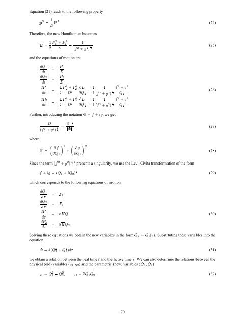
Equation (21) leads to the following property Ô ¾ ½ È¾ (24) Therefore, the new Hamiltonian becomes À ½ ¾ È ¾ ½ · È ¾ ¾ ½ ´ ¾ · ¾ µ ½ ¾ (25) and the equations of motion are É ½ Ø È ½ É ¾ Ø È ½ Ø È ¾ Ø È ¾ ½ È½ ¾ · È ¾ ¾ ¾ ¾ ½ ¾ È ¾ ½ · È ¾ ¾ ¾ É ½ É ¾ ½ ½ ¾ ´ ¾ · ¾ µ ¿ ¾ ½ ½ ¾ ´ ¾ · ¾ µ ¿ ¾ ¾ · ¾ (26) É ½ ¾ · ¾ É ¾ Further, introducing the notation ¨ · , we get ´ ¾ · ¾ µ ½ ¾ ¨¼ ¾ ¨ (27) where ¨¼ ¾ ¾ · (28) É ½ É ½ Since the term ´ ¾ · ¾ µ ½¾ presents a singularity, we use the Levi-Civita transformation of the form · ´É ½ · É ¾ µ ¾ (29) which corresponds to the following equations of motion É ½ É ¾ È ½ È ¾ È ½ È ¾ ÀÉ ½ (30) ÀÉ ¾ Solving these equations we obtain the new variables in the form É É ´ µ. Substituting these variables into the equation Ø ´É ¾ ½ · É¾ ¾ µ (31) we obtain a relation between the real time Ø and the fictive time ×. We can also determine the relations between the physical (old) variables (Õ ½ Õ ¾ ) and the parametric (new) variables (É ½ É ¾ ) Õ ½ É ¾ ½ É ¾ ¾ Õ ¾ ¾É ½ É ¾ (32) 70
4 Numerical Examples The above results will now be tested for the Kepler’s problem, which Hamiltonian is À Ô¾ ½ ¾ · Ô¾ ¾ ¾ ½ Ô Õ ¾ ½ · Õ¾ ¾ (33) where (Õ ½ , Õ ¾ ) are the conjugate coordinate and (Ô ½ , Ô ¾ ) are the conjugate momentum of the two bodies in the phase space. The equations of motion are Õ ½ Ø Õ ¾ Ø Ô ½ Ø Ô ¾ Ø Ô ½ Ô ¾ Õ ½ Ô´Õ ¾ ½ · Õ¾ ¾ µ¿ (34) Õ ¾ Ô ´Õ ¾ ½ · Õ¾ ¾ µ¿ First, we use the 4th (Ò ) order symplectic schema (SI4): Õ Õ ½ · Ô ½ (35) Õ Ô Õ ½ Õ ´Õ ½ ¾ · Õ ¾ ¾ µ ¿ where ´ µ is given by the equations (10). ½ ¾ ½ Figure 1: The numerical solution of the Kepler’s problem (SI4) In Figure 1 we present the numerical results of the Kepler’s problem (35), using the SI4 integrator. In this case, we chose the following initial conditions Õ ¼ ½ ¼¿¾, Ô¼ ½ ¼¼, Õ¼ ¾ ½¼¿½, Ô¼ ¾ ¼¿¿½, Ø ¼ ¼, Ø ¾¼. In Figure 2 we give the numerical results of the Kepler’s problem (34), using the 4th order Runge-Kutta (RK4) integrator with variable steps. The same initial conditions are used as in case of the Figure 1. In Figure 3 we show the results of computations using the regularization procedure, equation (30), and RK4 with variable steps. Now, the initial conditions are Õ½ ¼ ¼¾, Ô¼ ½ ½½¼, Õ¼ ¼¼, ¾ Ô¼ ½¿, Ø ¾ ¼ ¼, Ø ½¼. Next, we study the energy error ´Ô ¾ ½ · Ô¾ ¾ µ¾ ½Ô Õ½ ¾ · Õ¾ ¾ , which varies linearly with time using the RK4 method. It is assumed that it remains bounded and small for the SI4 (Figure 4). 71
Page 1 and 2: TECHNISCHE MECHANIK, Band 24, Heft
Page 3: 3 Regularization Procedure We shall
Page 7: 5 Conclusions In this paper symplec

Symplectic and Regularization Methods

You also want an ePaper? Increase the reach of your titles

Delete template?

Save as template?