Symplectic and Regularization Methods

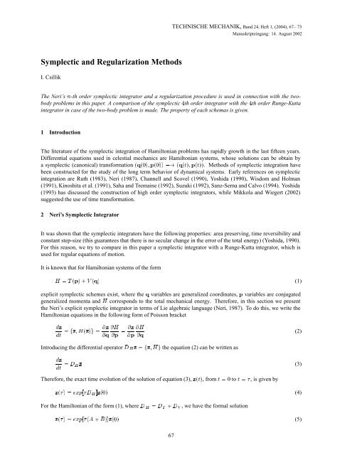
TECHNISCHE MECHANIK, Band 24, Heft 1, (2004), 67– 73
Manuskripteingang: 14. August 2002
Symplectic and Regularization Methods
I. Csillik
The Neri’s Ò-th order symplectic integrator and a regularization procedure is used in connection with the twobody
problems in this paper. A comparison of the symplectic th order integrator with the th order Runge-Kutta
integrator in case of the two-body problem is made. The property of each schemas is given.
1 Introduction
The literature of the symplectic integration of Hamiltonian problems has rapidly growth in the last fifteen years.
Differential equations used in celestial mechanics are Hamiltonian systems, whose solutions can be obtain by
a symplectic (canonical) transformation ´Õ´¼µ Ô´¼µµ ´Õ´Øµ Դصµ. Methods of symplectic integration have
been constructed for the study of the long term behavior of dynamical systems. Early references on symplectic
integration are Ruth (1983), Neri (1987), Channell and Scovel (1990), Yoshida (1990), Wisdom and Holman
(1991), Kinoshita et al. (1991), Saha and Tremaine (1992), Suzuki (1992), Sanz-Serna and Calvo (1994). Yoshida
(1993) has discussed the construction of high order symplectic integrators, while Mikkola and Wiegert (2002)
suggested the use of time transformation.
2 Neri’s Symplectic Integrator
It was shown that the symplectic integrators have the following properties: area preserving, time reversibility and
constant step-size (this guarantees that there is no secular change in the error of the total energy) (Yoshida, 1990).
For this reason, we try to compare in this paper a symplectic integrator with a Runge-Kutta integrator, which is
used for regular equations of motion.
It is known that for Hamiltonian systems of the form
À Ì ´Ôµ ·Î ´Õµ (1)
explicit symplectic schemes exist, where the Õ variables are generalized coordinates, Ô variables are conjugated
generalized momenta and À corresponds to the total mechanical energy. Therefore, in this section we present
the Neri’s explicit symplectic integrator in terms of Lie algebraic language (Neri, 1987). To do this, we write the
Hamiltonian equations in the following form of Poisson bracket
Þ
Ø
Þ À
ÞÀ´Þµ
Õ Ô
Þ À
Ô Õ
(2)
Introducing the differential operator À Þ ÞÀ the equation (2) can be written as
Þ
Ø À Þ (3)
Therefore, the exact time evolution of the solution of equation (3), ޴ص, from Ø ¼to Ø , is given by
Þ´ µÜÔ À ℄Þ´¼µ (4)
For the Hamiltonian of the form (1), where À Ì · Î , we have the formal solution
Þ´ µÜÔ ´ · µ℄Þ´¼µ (5)
67

where Ì and Î are two operators which do not commute. Further, we suppose that the set of the
real numbers ´ µ, ½Òsatiesfies the equality
ÜÔ ´ · µ℄
Ò
½
ÜÔ´ µ ÜÔ´ µ·Ç´ Ò·½ µ (6)
where Ò is the integrator’s order Trotter (1959). Let now a mapping from Þ Þ´¼µ to Þ ¼ Þ´ µ be given by
Þ ¼
Ò
½
ÜÔ´ µ ÜÔ´ µ
Þ (7)
This application is symplectic because it is a product of elementary symplectic mappings. We can write the explicit
equation (7) in the following form
Õ Õ ½ ·
Ì
Ô
ÔÔ ½
Î
Ô Ô ½ · ½Ò (8)
Õ ÕÕ
where Þ ´Õ ¼ Ô ¼ µ and Þ ¼ ´Õ Ò Ô Ò µ. This system of equations is an Ò-th order symplectic integration scheme.
The numerical coefficient , , ½Òare not uniquely determined from the requirement that the local truncation
error is of order Ò . If one requires the time reversibility of the numerical solution, one can determine it uniquely.
We present now two examples, the 1st (Ò ½) and the 4th (Ò ) order integrators. The 1st order integrator
schema is given by
Õ ½ Õ ¼ · ½
Ì
Ô
Ô ½ Ô ¼ · ½
Î
Õ
where ½ ½ ½.
ÔÔ ¼
(9)
ÕÕ ½
The 4th order integrator schema is rather long so that we present only the values of the coefficients ´ µ, ½ .
They are
½
½
¾´¾ ¾ ½ ¿ µ
¾ ¿ ½ ¾ ½ ¿
¾´¾ ¾ ½ ¿ µ
(10)
½ ¿ ½
¾ ¾ ½ ¿
¾ ½ ¿
¾
¾ ¾ ½ ¿
¼
We mention that Yoshida (1990) showed that the 4th order symplectic integrator is composed by 2nd order integrators
of the form
Ë ´Ì µË ¾´Ü ½ µË ¾´Ü ¼ µË ¾´Ü ½ µ (11)
where
Ë ¾´Ì µÜÔ ÜÔ ´µ ÜÔ
¾ ¾
(12)
The solution Ü ¼ and Ü ½ are determined from the algebraic equation
Ü ¼ ·¾Ü ½ ½ Ü ¿ ¼ ·¾Ü¿ ½ ¼ (13)
The hight order integrators ( ) have been generalized to arbitrary orders by Suzuki (1992).
68

3 Regularization Procedure
We shall now present a regularization procedure to study the effect of collision in the Kepler’s problem, which
describes the motion in the configuration plane of a material point that is attracted towards the origin with a force
inversely proportional to the distance squared.
À Ì · Î Ì ½ ¾ ´Ô¾ ½ · Ô¾µ Î ¾ ½
Ô
Õ
¾
½ · Õ¾ ¾
(14)
The regularization procedure is utilised when the particle approaches very closely (collision) the central mass and
produces large gravitational forces, and sharp bends of the orbit. The regularization originates from the singularity
given by the Hamiltonian function for Õ ¼. In this respect, we introduce the coordinate transformation
Ë ¿ Ô ½ ´É ½ É ¾ µ·Ô ¾ ´É ½ É ¾ µ (15)
where and are conjugate harmonic functions, which satisfy the Cauchy-Riemann relations
É ½ É ¾
É ¾
É ½
(16)
and ´É ½ É ¾ µ are the new conjugate coordinates. Using this relations, we can write
Õ Ë ¿
Ô
È Ë ¿
É
´ ½ ¾µ (17)
so that the transformed equations become
Õ ½ ´É ½ É ¾ µ
Õ ¾ ´É ½ É ¾ µ
È ½ Ô ½ · Ô ¾
(18)
É ½ É ¾
È ¾ Ô ½ · Ô ¾
É ¾ É ½
where ´È ½ È ¾ µ are the new conjugate momentum. To study the regularization, we introduce the notation
É ½
½½
É ½
½¾ (19)
Using this notation equations (18) become
È ½ ½½ Ô ½ · ½¾ Ô ¾ (20)
È ¾ ½¾ Ô ½ · ½½ Ô ¾
which can be written as
È ¡ Ô (21)
where
½½ ½¾
Ô½
Ô
½¾ ½½ Ô ¾
(22)
and
´É ½ É ¾ µØ
¾ ¾
·
(23)
É ½ É ½
69

Equation (21) leads to the following property
Ô ¾ ½ Ⱦ (24)
Therefore, the new Hamiltonian becomes
À ½ ¾
È ¾ ½ · È ¾ ¾
½
´ ¾ · ¾ µ ½ ¾
(25)
and the equations of motion are
É ½
Ø
È ½
É ¾
Ø
È ½
Ø
È ¾
Ø
È ¾
½ Ƚ ¾ · È ¾
¾
¾ ¾
½
¾
È ¾ ½ · È ¾ ¾
¾
É ½
É ¾
½ ½
¾
´ ¾ · ¾ µ ¿ ¾
½ ½
¾
´ ¾ · ¾ µ ¿ ¾
¾ · ¾
(26)
É ½
¾ · ¾
É ¾
Further, introducing the notation ¨ · , we get
´ ¾ · ¾ µ ½ ¾
¨¼ ¾
¨
(27)
where
¨¼
¾ ¾
·
(28)
É ½ É ½
Since the term ´ ¾ · ¾ µ ½¾ presents a singularity, we use the Levi-Civita transformation of the form
· ´É ½ · É ¾ µ ¾ (29)
which corresponds to the following equations of motion
É ½
É ¾
È ½
È ¾
È ½
È ¾
ÀÉ ½ (30)
ÀÉ ¾
Solving these equations we obtain the new variables in the form É É ´ µ. Substituting these variables into the
equation
Ø ´É ¾ ½ · ɾ ¾
µ (31)
we obtain a relation between the real time Ø and the fictive time ×. We can also determine the relations between the
physical (old) variables (Õ ½ Õ ¾ ) and the parametric (new) variables (É ½ É ¾ )
Õ ½ É ¾ ½ É ¾ ¾ Õ ¾ ¾É ½ É ¾ (32)
70

4 Numerical Examples
The above results will now be tested for the Kepler’s problem, which Hamiltonian is
À Ô¾ ½
¾ · Ô¾ ¾
¾
½
Ô
Õ
¾
½ · Õ¾ ¾
(33)
where (Õ ½ , Õ ¾ ) are the conjugate coordinate and (Ô ½ , Ô ¾ ) are the conjugate momentum of the two bodies in the
phase space. The equations of motion are
Õ ½
Ø
Õ ¾
Ø
Ô ½
Ø
Ô ¾
Ø
Ô ½
Ô ¾
Õ ½
Ô´Õ ¾ ½ · Õ¾ ¾ µ¿ (34)
Õ ¾
Ô
´Õ ¾ ½ · Õ¾ ¾ µ¿
First, we use the 4th (Ò ) order symplectic schema (SI4):
Õ Õ ½
· Ô ½
(35)
Õ
Ô Õ ½
Õ
´Õ ½
¾
· Õ
¾
¾ µ ¿
where ´ µ is given by the equations (10).
½ ¾ ½
Figure 1: The numerical solution of the Kepler’s problem (SI4)
In Figure 1 we present the numerical results of the Kepler’s problem (35), using the SI4 integrator. In this case, we
chose the following initial conditions Õ ¼ ½ ¼¿¾, Ô¼ ½ ¼¼, Õ¼ ¾ ½¼¿½, Ô¼ ¾ ¼¿¿½, Ø ¼ ¼, Ø ¾¼.
In Figure 2 we give the numerical results of the Kepler’s problem (34), using the 4th order Runge-Kutta (RK4)
integrator with variable steps. The same initial conditions are used as in case of the Figure 1.
In Figure 3 we show the results of computations using the regularization procedure, equation (30), and RK4 with
variable steps. Now, the initial conditions are Õ½ ¼ ¼¾, Ô¼ ½ ½½¼, Õ¼ ¼¼, ¾ Ô¼ ½¿, Ø ¾ ¼ ¼,
Ø ½¼. Next, we study the energy error ´Ô ¾ ½ · Ô¾ ¾ µ¾ ½Ô Õ½ ¾ · Õ¾ ¾
, which varies linearly with time using
the RK4 method. It is assumed that it remains bounded and small for the SI4 (Figure 4).
71

Figure 2: The numerical solution of the Kepler’s problem (RK4)
Figure 3: The numerical solution of the regularized two-body problem (RK4)
Figure 4: Energy conservation for the two-body problem
72

5 Conclusions
In this paper symplectic integrators (SI4) were compared with traditional integrators of Runge-Kutta type (RK4).
It is shown that the symplectic integrators have the merits to integrate the Hamiltonian systems over a very long
time. It is seen that the numerical solution does not distort the trajectory, but there is a precession effect (Figure 1).
Using regular differential equations the numerical precision is more efficient. This fact can be seen by comparing
the numerical results shown on Figures 1-3.
References
Channell, P. J.; Scovel, J. C.: Symplectic integration of hamiltonian systems. Nonlinearity, 3, (1990), 231 – 259.
Kinoshita, H.; Yoshida, H.; Nakai, H.: Symplectic integrators and their application to dynamical astronomy. Celestial
Mechanics, 50, (1991), 59 – 71.
Mikkola, S.; Wiegert, P.: Regularizing time transformations in symplectic and composite integration. Celestial
Mechanics and Dynamical Astronomy, 82, (2002), 375 – 390.
Neri, F.: Lie algebras and canonical integration. Dept. of Physics, Univ. of Maryland, preprint (1987).
Ruth, R. D.: A canonical integration technique. IEEE Trans. Nucl. Sci, NS, 30, (1983), 2669 – 2671.
Saha, P.; Tremaine, S.: Symplectic integrators for solar system dynamics. Astron. J., 104, (1992), 1633 – 1640.
Sanz-Serna, J. M.; Calvo, M. P.: Numerical hamiltonian problems. Chapman and Hall, London (1994).
Suzuki, M.: General theory of higher-order decomposition of exponential operators and symplectic integrators.
Phy. Lett. A, 165, (1992), 387 – 395.
Trotter, H. F.: On the product of semi-groups of operators. Proc. Am. Math. Phys., 10, (1959), 545–551.
Wisdom, J.; Holman, M.: Symplectic maps for the Ò-body problem. The Astronomical Journal, 102, (1991), 1528
– 1538.
Yoshida, H.: Construction of higher order symplectic integrators. Phys. Lett. A, 150, (1990), 262 – 268.
Yoshida, H.: Recent progress in the theory and application of symplectic integrators. Celestial Mechanics, 56,
(1993), 27 – 43.
Address: I. Csillik, Faculty of Mathematics and Computer Science, Babeş-Bolyai University, Cluj-Napoca, R-
3400, Ciresilor-19, Romania.
email: iharka@math.ubbcluj.ro.
73