Testing and quality

More documents

Recommendations

Info

TESTING AND QUALITY Revealing and interpreting hidden features using dedicated signal analysis Filter and fit Based on the signals of only a few sensors, Sulzer Innotec was successful in identifying the most important natural frequencies and vibration mode shapes of a pump impeller. The results are, essentially, in good agreement with the FEM calculations performed by Sulzer Pumps. The measurement results indicate that the mechanical resonances are quite well damped, so that they will not jeopardize the integrity of the impeller in any way. 1 Positions of strain gauges and accelerometers on the impeller (axial view) (Source: PhD. thesis by Stefan Berten) 14 | Sulzer Technical Review 1/2011 In 2009, Sulzer Innotec received an order from the Sulzer Pumps division to analyze and assess vibration signals measured in a pump test stand. The test pump that was examined is the reproduction of the last stage of a highpressure centrifugal pump operated by a variable-speed drive. This impeller stage has a rated power of 1.4MW. The impeller has seven blades and a diameter of 0.35m. In centrifugal pumps, rotor-stator interactions and flow separation phenomena are known to excite vibrations of stationary or rotating components, which might result in fatigue failure. Based on performance monitoring of a particular pump stage in part-load SG6 SG7 SG5 SG4 SG8 Acc3 Acc = Accelerometer SG = Strain gauge SG1 SG3 Acc1 Acc2 SG2 conditions, Sulzer Pumps assigned an extensive experimental investigation of the mechanical and hydraulic oscillations to the EPFL (École Polytechnique Fédérale de Lausanne). Many sensors for pressure, strain, acceleration, and displacement were installed in order to record the corresponding oscillations. All measurements were performed by the Laboratoire de Machines Hydrauliques (LMH) of the EPFL and analyzed, for the most part, in the context of a PhD. thesis. Customized analysis of the impeller mode shapes The task of Sulzer Innotec consisted of identifying the operational vibration mode shapes of the rotating impeller based on the measurement signals of the strain gauges and accelerometers installed on the impeller and assessing the results and comparing them with the results from FEM calculations. For certain operating conditions, a frequency excited by the stationary components might coincide with a weakly damped natural frequency of the impeller and might result in substantial resonance amplitudes. Conversely, a lack of strong resonant vibrations despite excitation at the resonance frequency indicates that the corresponding resonance is highly damped. The task of Sulzer Innotec was to analyze the vibration signals of two speed ramps—one run-up and one coastdown. Figure 1 indicates the positions of the eight strain gauges and three accelerometers installed on the impeller. Conditioning of strain gauge signals The recorded strain gauge signals were considerably affected by noise; substantial noise sources were sensor noise, bit noise of the analog digital converter ADC, and cross talk of external signals. The comparison of all strain gauge signals showed that these signals are mostly in phase and have similar amplitudes. The conclusion was that the signals were seriously affected by strong cross talk of an external signal. Therefore, as a first step of signal conditioning, the average value of all strain gauge signals was subtracted from each individual signal; thereby, the noise level could be substantially reduced. The resulting spectrograms now revealed the typical series of order lines, which result from the excitation at integer multiples of the pump rotation frequency. In particular, the orders 12, 24, and 36 are clearly prominent, as expected for a pump equipped with 12 diffuser guide vanes. 4330
Acceleration (g) 40 30 20 10 0 –10 –20 –30 –40 –50 –60 0 10 20 30 40 Time (s) 50 60 70 2 Time traces of accelerometers showing implausible excursions in negative direction and clipping at –50 g. Signals of the accelerometer The accelerometer signals were not optimal either (see 2); they showed numerous implausible excursions in the negative direction and substantial clipping at approximately –50g. Nevertheless, in the frequency domain, the results obtained with the accelerometers were quite well defined compared with the results from strain gauges and were therefore used for further investigations. Resonance detection using spectrograms Spectrograms are a common method for displaying characteristics of transient vibration signals. Figure 3 shows an 2500 2000 1500 Frequency (Hz) 3000 1000 500 Example 1: f = 1150 Hz (2-diameter mode, excitation by 23rd order) Example 2: f = 900 Hz (0-diameter mode, excitation by 21st order) example. The vibration levels are color coded and displayed as a function of time (= x-axis) and frequency (= y-axis). In the spectrogram of an accelerometer signal depicted in 3, the impeller natural frequencies are evident as horizontal, slightly fanned-out yellow-red shades (marked with red arrows in 3). The frequency bandwidth of the yellow-red shades is more than 100 Hz wide, indicating that the corresponding resonances feature considerable damping. A resonance with low damping would be evident by a rather narrow resonance bandwidth; no such feature crops up in the spectrogram of 3. Wherever the fanlike excitation frequencies of the rotor- 0 10 20 30 40 Time (s) 50 60 70 5-D 3 Spectrogram of the accelerometer signal Acc1 (Ramp with decreasing speed; frequency bands indicating resonances (yellow-red shades) marked by red arrows, resonances coinciding with a speed order line (circled in blue). 4-D 3-D 2-D 0-D 1-D Deflection (–) 1.0 0.8 0.6 0.4 0.2 0 –0.2 –0.4 –0.6 –0.8 –1.0 stator interaction coincide with a natural frequency of the impeller (see bluecircled lines), the corresponding resonance is excited. However, thanks to substantial damping, the amplification of the amplitude is not significant, and no fatigue damage is expected due to these resonances. Deflection shape identification It is well known that any given excitation order of the stationary components can excite only certain mode shapes of the impeller (Tanaka, 1990). Once the resonance frequencies of the impeller have been identified from the spectrogram, measured data and theoretically computed rotor vibrations can be matched in order to determine the corresponding mode shapes of the impeller. Following are two examples: • Example 1: Two-diameter mode at f=1150 Hz excited by the 23rd order: The frequency response function between two accelerometer signals is computed and averaged for the time segment in which a certain resonance mode is excited by the suitable excitation order. Then, the ratio of vibration amplitudes and the phase difference can be determined at the resonance frequency (f = 1150 Hz); at this frequency, the coherence should be reasonably good. The amplitude ratios and the relative phase at the measurement points are then animated synchronously with the theoretical vibration mode shape, the amplitude and phase of which are manually adapted to match the measured data. 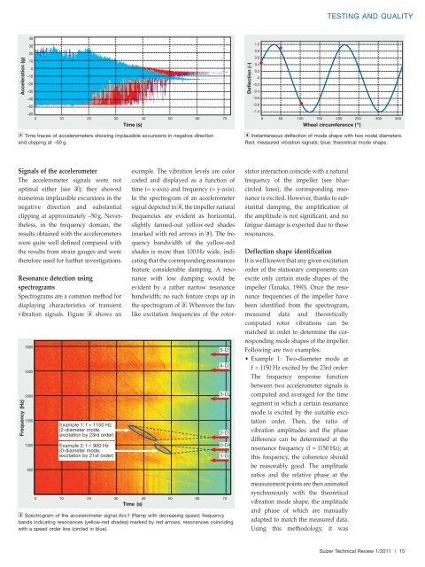Using this methodology, it was TESTING AND QUALITY 0 50 100 150 200 250 300 350 Wheel circumference (º) 4 Instantaneous deflection of mode shape with two nodal diameters. Red: measured vibration signals; blue: theoretical mode shape. Sulzer Technical Review 1/2011 | 15
Page 1 and 2: 1/2011 Proven quality Innovation th
Page 3 and 4: Testing and quality Panorama 4 News
Page 5 and 6: Shell Global Solutions and Sulzer C
Page 7 and 8: year, the test setup needs to be st
Page 9 and 10: ment as a function of suction press
Page 11 and 12: teristics such as apparent density,
Page 13: Nevertheless, a global approach is
Page 17 and 18: SULZER ANALOGY Testing poisons In t
Page 19 and 20: A product development process at Su
Page 21 and 22: simpler from the viewpoint of the
Page 23 and 24: provides a database, which, by revi
Page 25 and 26: SULZER INNOVATION The ideal solutio
Page 27 and 28: approximately to that of the pump,
Page 29 and 30: 6 Some HPRT trains are so long that
Page 31 and 32: distribution remains constant. On t
Page 33 and 34: SULZER WORLD Welcome to Sulzer Pump
Page 35 and 36: anches serve niche markets and, the

Testing and quality

Create successful ePaper yourself

Delete template?

Save as template?