Topic 2: The pendulum

PHY321F — cp 2005 24
Topic 2:
The pendulum
Here we enlarge upon the simple solution of a differential equation in Topic 1,
and apply it to a simple mechanical system. This solution, of course, depends
on knowledge of an initial position and velocity: it is an initial value problem.
2.1 Description of problem
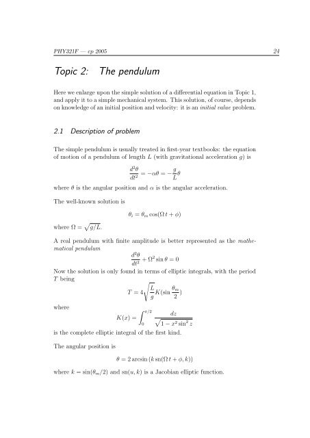
The simple pendulum is usually treated in first-year textbooks: the equation
of motion of a pendulum of length L (with gravitational acceleration g) is
d 2 θ
dt 2 = −αθ = − g L θ
where θ is the angular position and α is the angular acceleration.
The well-known solution is
where Ω = √ g/L.
θ i = θ m cos(Ω t + φ)
A real pendulum with finite amplitude is better represented as the mathematical
pendulum
d 2 θ
dt + 2 Ω2 sin θ = 0
Now the solution is only found in terms of elliptic integrals, with the period
T being
where
T = 4
K(x) =
√
∫ π/2
0
L
g K(sin θ m
2 )
dz
√
1 − x2 sin 2 z
is the complete elliptic integral of the first kind.
The angular position is
θ = 2 arcsin (k sn(Ω t + φ, k))
where k = sin(θ m /2) and sn(u, k) is a Jacobian elliptic function.

PHY321F — cp 2005 25
The problem of determining the position as a function of time, or the period,
is now a matter of finding the value of some elliptic integrals. As there is
no ‘calculator key’ for these, we either have to interpolate from tables or
evaluate the integrals numerically. These are both computational problems.
We can, of course, also solve the differential equation on the computer.
We can make the pendulum model more realistic by including damping. The
linearly damped harmonic oscillator and its solution are well-known:
d 2 θ
dt + 2 Ω2 θ + β dθ
dt = 0
where β = b/(mL) with b a damping parameter and m the bob mass. Then
the solution is
θ = θ m e − β 2 t cos(Ω t + φ)
Of course we should really do this for the mathematical pendulum — then
there is no analytical solution. In addition, the damping term is inappropriate
for a pendulum bob moving at a typical speed in air. The damping force is
better described by
F d = 1 2 CρAv|v|
(where ρ is the density of air, C is a drag coefficient, A an effective crosssectional
area and v is the speed L ˙θ of the bob) rather than F d = bv. C can
depend on the speed as well. This gives a drag term in the above equation
C dθ
ρAL
2m dt
dθ
∣ dt ∣ = γ dθ
dθ
dt ∣ dt ∣
Let us see how to solve this problem computationally.
2.2 Numerical methods
2.1 Solving the differential equation
While there exist techniques for integrating second-order differential equations,
it is more convenient to exploit first-order integrators. We start by
writing the basic equation (without damping) we want to solve as a system

PHY321F — cp 2005 26
of two coupled first order equations:
dω
dt = −Ω2 sin θ (5)
dθ
dt = ω (6)
where ω is the angular velocity and θ is the angular position.
These equations can now be integrated using the Euler method.
Suppose we know the position and velocity at a time t = i∆t. Then the
above pair of coupled equations can be rewritten as
ω i+1 = ω i − ∆t Ω 2 sin θ i (7)
θ i+1 = θ i + ∆t ω i (8)
(Note that this method can obviously be generalised to solve an arbitrary
system of equations
dy i
dt = f i(y 1 , y 2 , . . . , y N , t)
i = 1, . . . , N
which can be written in a vector notation
dy
dt
= f(y, t)
This is the equation typically solved by a real ODE integrator.)
Write a program (see example) to solve equations (3) and (4), and check that
the result for small initial angular displacement is what you expect.
This solution suffers from a defect: the computed solution does not conserve
the energy E = 1 2 mL2 ω 2 +mgL(1−cos θ). Change your program to calculate
the energy and show this.
A slight modification, however, gives a system which does conserve energy.
ω i+1 = ω i − ∆t Ω 2 sin θ i (9)
θ i+1 = θ i + ∆t ω i+1 (10)
This Euler-Cromer method is a first order area-preserving mapping. Such
mappings exploit the symplectic structure of Hamilton’s equations — they
preserve the canonical structure of these equations.

PHY321F — cp 2005 27
However, this cannot be so easily generalised. The Euler method is an example
of an explicit method. The new value can be determined by stepping
from the old value. By contrast, the Euler-Cromer method is implicit — the
expression for the new value contains the new value, and thus constitutes
a system of equations to be solved for that value, rather than a simple assignment.
This solution is trivial in the Euler-Cromer case, but is not so in
general.
Including the air drag term in, say, the Euler solution gives:
ω i+1 = ω i − ∆t(Ω 2 sin θ i + γ ω i |ω i |) (11)
θ i+1 = θ i + ∆t ω i (12)
2.3 Computation
Here is a simple Python program using the Euler method.
from Numeric import *
g=9.81 # m/s**2
l=1.00 # length in m
Nsteps = 100
w0sq = g/l
dt=0.1
vn=0.0
xn=30.0*pi/180.0
# time step
# initial speed zero at extreme posn.
# initial angular position 30 degrees
for i in range(Nsteps+1):
print i, xn, vn
vnp1 = vn - w0sq*sin(xn)*dt
xnp1 = xn + vn*dt # Euler
xn = xnp1
vn = vnp1

PHY321F — cp 2005 28
2.4 Higer-order methods
Better accuracy is achieved in a single time-step by using a higher-order
integration method. These typically use more derivative information to gain
accuracy.
A simple example is (velocity) Verlet method. (There are other Verlet methods
equivalent mathematically although not necessarily numerically).
θ i+1 = θ i + ω i ∆t + 1 2 a i (∆t) 2
ω i+1 = ω i + 1 2 (a i + a i+1 ) ∆t
This method also has the advantage of preserving energy conservation.
Aother second order method is the Euler-Richardson method which uses the
slope in the middle of the time-step for extrapolation to the next point. This
results in O(∆t) 2 accuracy, at the expense of a second force evaluation.
a i = α(θ i , ω i , t i )
ω mid = ω i + a i
∆t
2
θ mid = θ i + ω i
∆t
2
a mid = α(θ mid , ω mid , t i + ∆t
2 )
ω i+1 = ω i + a mid ∆t
θ i+1 = θ i + ω mid ∆t
This is essentially a second order Runge-Kutta method and can be derived
in several ways. It can be combined with the standard Euler step to obtain
information on the truncation error. With this the method can easily be
extended to offer adaptive control: the step-size can be varied to maintain
an error limit.
2.5 Exercises
1. Compare the Euler and Euler-Cromer methods of integration.
2. Determine the dependence of the frequency of the pendulum on its
amplitude. One possible means of analysis is to determine the power
spectrum of the oscillations from the Fourier transform of the solution.

PHY321F — cp 2005 29
You will need to compute the solution as an array of values and take
the FFT of the result.
3. Include the drag force term in your solution. Assume the pendulum
consists of a 1.0 cm diameter steel ball bearing suspended 1.0 m from
the pivot, and is started from an angle of 40.0 ◦ . How long will it take
for the amplitude to decrease to 5.0 ◦ ? (See e.g. Halliday and Resnick
for drag coefficients and air density). Interestingly, the Euler solution
might be better than Euler-Cromer for this case.
4. Program the case of linear damping. Compare the decrease in energy
of the pendulum using the Euler and Euler-Cromer methods. How do
they agree with the analytical solution?
2.6 Literature
1. Stable solutions using the Euler approximation. A. Cromer, Am. J.
Phys. 49 455-459 (1981).
2. The pendulum — rich physics from a simple system. R.A. Nelson and
M.G. Olsson, Am. J. Phys. 54 112-121 (1986).
3. Numerical integration of Newton’s equations including velocity-dependent
forces. I.R. Gatland, Am. J. Phys. 62 259-265 (1994).

PHY321F — cp 2005 30
D
A digression: Ordinary differential equations
D.1 Explicit and implicit methods
Consider an equation of the form
dy(x)
dx
The explicit Euler-method solution is
= −λ y(x)
y(x + h) = (1 − h λ)y(x)
(where we use now a generic variable x and stepsize h).
This solution is unstable if h > 2/λ. We can see this by considering the error
e(x), i.e. the difference between the true solution ŷ(x) and the computed
solution y(x), Then
e(x + h) ≈ e(x)(1 − h λ)
This error term grows if |1 − h λ| > 1.
This can be compared to an implicit scheme
y(x + h) = y(x) − h λ y(x + h)
= y(x)
1 + h λ
Note that we have to solve an equation in order to obtain y(x + h). In this
case, the solution is trivial, but in more complicated cases, the solution could
involve substantial numerical effort.
However, the stability is now assured as
e(x + h) ≈
e(x)
1 + h λ
so that the error term decreases for all h > 0.
Implicit equations are important in the solution of stiff systems, where a
rapidly decaying part of the solution dominates the stability.

PHY321F — cp 2005 31
D.2 Runge-Kutta methods
The simple methods we have considered are only correct to first order in h.
Obviously, higher order methods can be expected to offer benefits (although
this might not extend to accuracy).
One way of generating such methods leads to a class of Runge-Kutta methods.
By way of example, suppose we solve a system
by the Euler method to get
dy(x)
dx
= f(x, y)
y(x + h) = y(x) + h f(x, y)
The derivative over the interval of size h is taken from the initial point. A
better value, perhaps, would be to take the value at the centre of the interval.
The value of y at the centre of the interval can be estimated from the above
Euler step This then gives a solution
k 1 = h f(x, y(x))
k 2 = h f(x + h 2 , y(x) + 1 2 k 1)
y(x + h) = y(x) + k 2
This method turns out to be second order, so that the error term is O(h 3 )
This process can be continued: the classic Runge-Kutta scheme is the fourth
order formula
k 1 = h f(x, y(x))
k 2 = h f(x + h 2 , y(x) + 1 2 k 1)
k 3 = h f(x + h 2 , y(x) + 1 2 k 2)
k 4 = h f(x + h 2 , y(x) + k 3)
y(x + h) = y(x) + k 1
6 + k 2
3 + k 3
3 + k 4
6
This is easily programmed, and thus is often used as a workhorse fixedstepsize
integration formula.

PHY321F — cp 2005 32
More control over the process is achieved if the error can be monitored. Suppose
we have two Runge-Kutta formulae, with solutions y(x + h) of order
h n+1 and ŷ(x + h) of order h n , Then the difference y − ŷ gives an estimate
of the error in y. This is especially useful if we can obtain both y and ŷ
from the same set of Runge-Kutta steps. (Such formulae are known as embedded
Runge-Kutta formulae; the additional work does not take additional
expensive evaluations of the function f).
Once we have an estimate of the error, it can be used to control the stepsize
so that some maximum error per step is not exceeded. This leads to a set
of adaptive Runge-Kutta methods. A modern adaptive RK code is rksuite
(or rksuite90), available from netlib.
D.3 Other methods
D.3.1
Predictor-corrector methods
The Euler and Runge-Kutta methods extrapolate from one point to the next.
Higher accuracy can be obtained by using several previous steps. These multistep
methods are usually implemented as predictor-corrector schemes. An
extrapolation is made to the next point using an explicit multistep formula.
The value obtained is then used in an implicit multistep formula to correct
this prediction. This scheme also permits error control by adaptive step
sizing. A standard PC code is vode (and related codes), available from
netlib.
These methods give high accuracy integrators, but are more complicated and
fussy to program than RK.
D.3.2
Extrapolation methods
Burlisch-Stoer methods (see, e.g. Numerical Recipes) use Richardson extrapolation
to the limit h → 0 in order to improve accuracy. Press. et. al seem to
think that these methods are about to replace PC methods (if they haven’t
already). Others disagree.

PHY321F — cp 2005 33
D.3.3
Symplectic methods
These are special methods for integrating Hamilton’s equations of motion.
They preserve the structure of these equations (or at least something close
by) and are much in vogue in the study of dynamical systems (e.g. chaos),
tracking codes for charged particle optics, etc. The Euler-Cromer method is
a simple example.

PHY321F — cp 2005 34
E
Fourier transforms
Fourier analysis forms the foundation of many powerful computational techniques.
This section is only a bare introduction.
E.1 Fourier series
Any periodic function f(t) = f(t + T ) can be expanded in the Fourier series:
∞∑
f(t) = c n e inωt
n=−∞
where ω = 2π/T .
The Fourier coefficients c n are obtained from
c n = 1 T
∫ T/2
−T/2
f(t) e −inωt dt
E.2 Fourier transform
Under fairly general conditions function f(t) can be expressed as a Fourier
transform:
f(t) = √ 1 ∫ ∞
F (ω) e iωt dω
2π
where
−∞
F (ω) = 1 √
2π
∫ ∞
−∞
f(t) e −iωt d t
This may be written F (ω) = F[f(t)] and f(t) = F −1 [F (ω)]
One speaks of transforming between the time and frequency domains.
E.3 Discrete Fourier transform
Let ∆ω = 2π/T .

PHY321F — cp 2005 35
The Fourier transform can be approximated by a discrete Fourier transform
(DFT). The time or frequency axes are replaced by a finite set of N points
on a grid and the integral performed using the trapezoidal rule:
F (n∆ω) ≈
=
N−1
∑
m=0
N−1
∑
m=0
f(m∆t) e −in∆ωm∆t
f(m∆t) e −i2πnm/N
The inverse transform is then
f(m∆t) = 1 N
N−1
∑
n=0
F (n∆ω) e i2πmn/N
Aliasing occurs for frequencies higher than the Nyquist frequency ω ny =
N∆ω/2 = (2π/∆t)/2
E.4 The fast Fourier transform
The importance of Fourier methods in computation derives from the existence
of the fast Fourier transform (FFT) algorithm, which is, well, a fast
way of computing the DFT. (What does fast mean? The DFT requires
O(N 2 ) calculations to compute the transform of N values; the FFT requires
O(N log N) — when N is of the order of 10 3 , a typical value, the FFT is
about 1000 times faster than the DFT. . . )
The FFT is a non-trivial algorithm and we won’t discuss it here — we’ll just
make use of a packaged version.
E.5 The fast Fourier transform in Python
In Python we can use:
from Numeric import *
from FFT import * # In windows : from Fft

PHY321F — cp 2005 36
...
F=fft(f) # f is a Numeric array
g=inverse_fft(F)
Note that F and g will be complex.
Application of the FFT is complicated slightly by the conventions used to
structure the data (Note that these are not peculiar to Python).
Suppose that the initial data f(t) is in the time domain, with N points at
a spacing δt, with T = Nδt. The transformed data F (ω) is (a) complex,
and (b) runs over the range −(N/2)δω . . . (N/2)δω, with δω = 2π/T . In
addition, the values coresponding to positive frequencies are returned in the
first half of the array, while those at negative frequencies in the second half of
the array. If the initial data has negative times, the same convention should
be applied.
E.6 Uses of the FFT
There are a number of applications of the FFT, based on various theorems
on Fourier transforms.
E.6.1
Power spectrum
The power spectrum gives essentially the intensity of the time-domain data
as a function of frequency.
It is defined by
and may be computed by
P (ω) = |F (ω)| 2
transform=fft(data) # transform is complex
powerspectrum=abs(transform*conjugate(transform))/len(data)**2
A single frequency in the data will result in a delta function in the power
spectrum. However, the FFT is always applied to a finite domain, and this
causes ‘power’ to leak to adjacent frequencies. Hence the delta function is

PHY321F — cp 2005 37
spread into a peak of finite width. The spread can be shaped by ‘windowing’
the data. See, e.g. Numerical Recipes for further information.
E.6.2
Convolution
The convolution f ∗ g of f(t) and g(t) is defined by
f ∗ g =
∫ ∞
−∞
f(τ) g(t − τ)dτ
By the convolution theorem,
F[f ∗ g] = F[f]F[g]
This provides a fast convolution algorithm via the FFT.
E.6.3
Correlation
The correlation corr(f, g) of f(t) and g(t) is defined by
corr(f, g) = 1 √
2π
∫ ∞
−∞
f ∗ (τ) g(t + τ)dτ
From the Fourier transforms F (ω) = F[f(t)] and G(ω) = F[g(t)],
F[corr(f, g)] = F ∗ (ω)G(ω)
The Wiener-Khinchine theorem relates the autocorrelation of a function to
the power spectrum:
F[corr(f, f)] = |F (ω)| 2