
You also want an ePaper? Increase the reach of your titles
YUMPU automatically turns print PDFs into web optimized ePapers that Google loves.
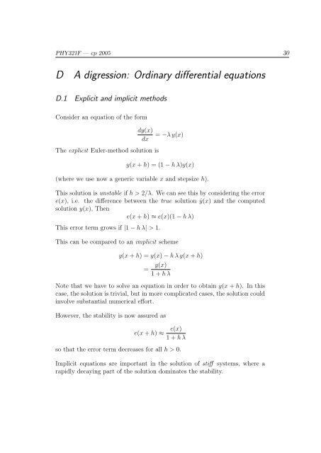
PHY321F — cp 2005 30<br />
D<br />
A digression: Ordinary differential equations<br />
D.1 Explicit and implicit methods<br />
Consider an equation of the form<br />
dy(x)<br />
dx<br />
<strong>The</strong> explicit Euler-method solution is<br />
= −λ y(x)<br />
y(x + h) = (1 − h λ)y(x)<br />
(where we use now a generic variable x and stepsize h).<br />
This solution is unstable if h > 2/λ. We can see this by considering the error<br />
e(x), i.e. the difference between the true solution ŷ(x) and the computed<br />
solution y(x), <strong>The</strong>n<br />
e(x + h) ≈ e(x)(1 − h λ)<br />
This error term grows if |1 − h λ| > 1.<br />
This can be compared to an implicit scheme<br />
y(x + h) = y(x) − h λ y(x + h)<br />
= y(x)<br />
1 + h λ<br />
Note that we have to solve an equation in order to obtain y(x + h). In this<br />
case, the solution is trivial, but in more complicated cases, the solution could<br />
involve substantial numerical effort.<br />
However, the stability is now assured as<br />
e(x + h) ≈<br />
e(x)<br />
1 + h λ<br />
so that the error term decreases for all h > 0.<br />
Implicit equations are important in the solution of stiff systems, where a<br />
rapidly decaying part of the solution dominates the stability.