Modeling Climate Policy Instruments in a Stackelberg Game with ...

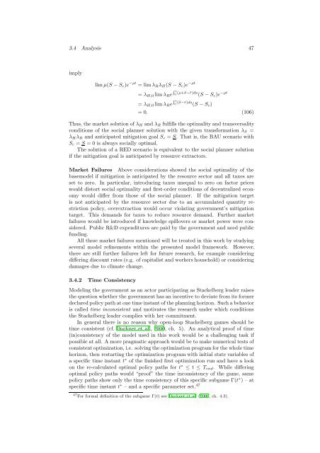
3.4 Analysis 47
imply
lim µ(S − S c )e −ρt = limλ R λ H (S − S c )e −ρt
= λ H,0 lim λ R e R t
0 (ρ+δ−¯r)ds (S − S c )e −ρt
= λ H,0 lim λ R e R t
0 (δ−¯r)ds (S − S c )
= 0. (106)
Thus, the market solution of λ H and λ R fulfills the optimality and transversality
conditions of the social planner solution with the given transformation λ S =
λ H λ R and anticipated mitigation goal S c = S. That is, the BAU scenario with
S c = S = 0 is always socially optimal.
The solution of a RED scenario is equivalent to the social planner solution
if the mitigation goal is anticipated by resource extractors.
Market Failures Above considerations showed the social optimality of the
basemodel if mitigation is anticipated by the resource sector and all taxes are
set to zero. In particular, introducing taxes unequal to zero on factor prices
would distort social optimality and first-order conditions of decentralized economy
would differ from those of the social planner. If the mitigation target
is not anticipated by the resource sector due to an accumulated quantity restriction
policy, overextraction would occur violating government’s mitigation
target. This demands for taxes to reduce resource demand. Further market
failures would be introduced if knowledge spillovers or market power were considered.
Public R&D expenditures are paid by the government and need public
funding.
All these market failures mentioned will be treated in this work by studying
several model refinements within the presented model framework. However,
there are still further failures left for future research, for example considering
differing discount rates (e.g. of capitalist and workers household) or considering
damages due to climate change.
3.4.2 Time Consistency
Modeling the government as an actor participating as Stackelberg leader raises
the question whether the government has an incentive to deviate from its former
declared policy path at one time instant of the planning horizon. Such a behavior
is called time inconsistent and motivates the research under which conditions
the Stackelberg leader complies with her commitment.
In general there is no reason why open-loop Stackelberg games should be
time consistent (cf. Dockner et al., 2000, ch. 5). An analytical proof of time
(in)consistency of the model used in this work would be a challenging task if
possible at all. A more pragmatic approach would be to make numerical tests of
consistent optimization, i.e. solving the optimization program for the whole time
horizon, then restarting the optimization program with initial state variables of
a specific time instant t ∗ of the finished first optimization run and have a look
on the re-calculated optimal policy paths for t ∗ ≤ t ≤ T end . While differing
optimal policy paths would “proof” the time inconsistency of the game, same
policy paths show only the time consistency of this specific subgame Γ(t ∗ ) – at
specific time instant t ∗ – and a specific parameter set. 47
47 For formal definition of the subgame Γ(t) see Dockner et al. (2000, ch. 4.3).