Lecture Notes on Compositional Data Analysis - Sedimentology ...

22 Chapter 4. Coordinate representation
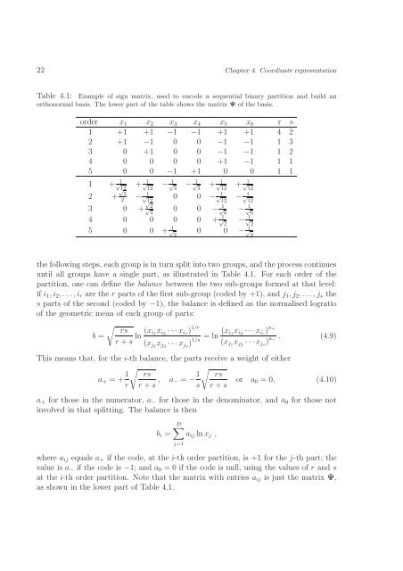
Table 4.1: Example of sign matrix, used to encode a sequential binary partition and build an
orthonormal basis. The lower part of the table shows the matrix Ψ of the basis.
order x 1 x 2 x 3 x 4 x 5 x 6 r s
1 +1 +1 −1 −1 +1 +1 4 2
2 +1 −1 0 0 −1 −1 1 3
3 0 +1 0 0 −1 −1 1 2
4 0 0 0 0 +1 −1 1 1
5 0 0 −1 +1 0 0 1 1
1 + 1 √
12
+ 1 √
12
− 1 √
3
− 1 √
3
+ 1 √
12
+ 1 √
12
2 + √ 3
2
− 1 √
12
0 0 − 1 √
12
− 1 √
12
3 0 + √ 2 √
3
0 0 − 1 √
6
− 1 √
6
4 0 0 0 0 + √ 1 2
− √ 1
2
5 0 0 + √ 1 2
0 0 − √ 1
2
the following steps, each group is in turn split into two groups, and the process continues
until all groups have a single part, as illustrated in Table 4.1. For each order of the
partition, one can define the balance between the two sub-groups formed at that level:
if i 1 , i 2 , . . .,i r are the r parts of the first sub-group (coded by +1), and j 1 , j 2 , . . .,j s the
s parts of the second (coded by −1), the balance is defined as the normalised logratio
of the geometric mean of each group of parts:
√ rs
b =
r + s ln (x i 1
x i2 · · ·x ir ) 1/r
(x j1 x j2 · · ·x js ) = ln (x i 1
x i2 · · ·x ir ) a +
1/s (x j1 x j2 · · ·x js ) a . (4.9)
−
This means that, for the i-th balance, the parts receive a weight of either
a + = + 1 √ rs
r r + s , a − = − 1 √ rs
or a 0 = 0, (4.10)
s r + s
a + for those in the numerator, a − for those in the denominator, and a 0 for those not
involved in that splitting. The balance is then
b i =
D∑
a ij ln x j ,
j=1
where a ij equals a + if the code, at the i-th order partition, is +1 for the j-th part; the
value is a − if the code is −1; and a 0 = 0 if the code is null, using the values of r and s
at the i-th order partition. Note that the matrix with entries a ij is just the matrix Ψ,
as shown in the lower part of Table 4.1.